Sharif University of Technology
Scientia IranicaTransaction F: Nanotechnology www.scientiairanica.com
Optimal sliding mode control for atomic force
microscope tip positioning during nano-manipulation
process
H. Babahosseini
a, S.H. Mahboobi
b, M. Khorsand Vakilzadeh
c, A. Alasty
cand A. Meghdari
c;a. Department of Mechanical Engineering, Virginia Tech, Blacksburg, VA, USA. b. Department of Bioengineering, University of California, Berkeley, CA, USA.
c. Center of Excellence in Design, Robotics and Automation, School of Mechanical Engineering, Sharif University of Technology, Tehran, Iran.
Received 21 June 2011; received in revised form 1 December 2012; accepted 21 January 2013
KEYWORDS AFM-based nanomanipulation; Nanoscale interaction forces;
Optimal nonlinear control.
Abstract. This research presents two-dimensional controlled pushing-based nanoma-nipulation using an Atomic Force Microscope (AFM). A reliable control of the AFM tip position is crucial to AFM-based manipulation since the tip can jump over the target nanoparticle causing the process to fail. However, detailed modeling and an understanding of the interaction forces on the AFM tip have a central role in this process. In the proposed model, the Lund-Grenoble (LuGre) method is used to model the dynamic friction force between the nanoparticle and the substrate. This model leads to the stick-slip behavior of the nanoparticle, which is in agreement with the experimental behavior at nanoscale. Derjaguin interaction force, which includes both attractive and repulsive interactions, is used to model the contact between the tip and nanoparticle. AFM is modeled by the lumped-parameter model. A controller is designed based on the proposed dynamic model for positioning of the AFM tip during a desired nanomanipulation task. An optimal sliding mode approach is used to design the controller, and the performance of the controller is shown by the simulation.
c
2013 Sharif University of Technology. All rights reserved.
1. Introduction
Recently, the Atomic Force Microscope (AFM) has evolved into a promising tool for micro/nanoparticles manipulation and assembly [1]. A controlled AFM probe, as a pushing manipulator, is able to position the micro/nanoparticles in a two-dimensional space to build miniaturized structures [1,2]. A precise controller that guarantees a stable and accurate tip positioning, is essential for nanomanipulation.
*. Corresponding author. Tel.: +98 21 66165541; Fax:+98 21 66000021
E-mail address: [email protected] (A. Meghdari)
Thus far, some control schemes have been de-signed to make the AFM tip track a certain trajectory for the manipulation task. Delnavaz et al. [1] proposed a combined classical and second order sliding mode for vibration suppression of the AFM tip in nanomanip-ulation tasks, while the AFM has been modeled by a mass-spring-damper system. In addition, Rai et al. [3] established a robust adaptive controller for AFM tip positioning. In this reference, the proposed modeling includes the coupled dynamics of the microcantilever and piezotube actuator. Uncertainties due to the probe-sample contact are considered in the model.
In this paper, an optimal sliding mode approach is proposed to control the AFM probe as a nonlinear
sys-tem. This approach displays a satisfactory performance and robustness to model uncertainties, while having a simple control structure. To obtain an optimal control response, slope tuning of the sliding mode surface, which is a complex task, is done by the LQ method [4]. During manipulation, the tip-particle-substrate system experiences complicated dynamics. A perfect model of nanomanipulation is crucial for a successful control, and, so far, several research studies have been conducted to model AFM-based nanomanipulation [5-9]. Most of these works have applied static friction models that have shortcomings and are not proper for nanoscale phenomena. Tafazzoli et al. [5-7] proposed a model of the AFM-based lateral nanomanipulation process. They used a traditional coulomb friction model with an additional modifying term as the nano-friction force. This nano-friction force reproduces a steady sliding response of the nanoparticle, which is usually observed in the macroscale. The dynamic behavior of a nanoparticle during AFM-based pushing is studied in [10,11]. The model is composed of the LuGre fric-tional sub-model, which leads to the stick-slip behavior of the nanoparticle. Some studies have used molecular dynamics to investigate the behaviors of the nano-particle during nanomanipulation [12,13].
The remainder of the paper is organized as fol-lows. In Section 2, the nanomanipulation modeling is presented. A new sliding mode control approach, optimized by the Linear Quadratic (LQ) method, is introduced in Section 3 and an optimal nonlinear controller is designed to suppress the vibration of the AFM microcantilever and make the tip track the specied trajectory. Finally, simulation results are illustrated and the conclusion is drawn in Sections 4 and 5, respectively.
2. Nanomanipulation modeling
AFM-based nanomanipulation modeling can be di-vided into two subsystems: the AFM dynamic model and the dynamic model of the nanoparticle. Also, three important phenomena, including nanoscale interaction forces, contact mechanics, and nanoscale friction force, are coupled in the dynamical model. The following sections will be devoted to presenting a suitable model of the AFM and the nanoparticle during manipula-tion.
2.1. AFM model
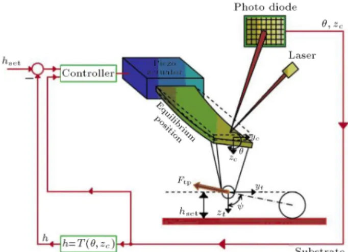
The Atomic Force Microscope (AFM) system is a promising tool for nanomanipulation. The AFM pro-vides additional capabilities and advantages compared to other manipulators; especially its ability to manipu-late metallic nanoparticles in every environment. The AFM pushes the individual nanoparticle by exerting direct force on it in the desired direction. A typical
AFM system consists of a piezoelectric actuator and a microcantilever chip with a sharp tip mounted on the piezoelectric. A position sensitive photo detector comes with the system, which receives a laser beam reected from the end point of the microcantilever to provide its deection feedback [14].
The current AFM model is based on a lumped-parameters modeling approach [5,15]. The AFM can-tilever is modeled as a 3-Degree Of Freedom (DOFs) mass-spring system. The springs include a linear spring to account for the normal deections and a torsional spring for the lateral twisting of the probe. The lateral deection of the microcantilever is not considerable, so, it is ignored [5]. The microcantilever has Young's modulus, E, shear modulus, G, length, L, width, w, and thickness, t. The stiness coecients of the springs, kand kz, can be calculated as:
k= Ewt 3
6L(1 + ); (1)
kz =Ewt 3
4L3 : (2)
The force (Fz) and moment (M) of the springs are
proportional to the vertical deformation (zc) and the
torsional angle (), respectively:
Fz= kz:zc; (3)
M= k:: (4)
A rigid AFM tip is also attached to the microcantilever lumped model. Figure 1 depicts a free body diagram of the AFM lumped-parameters model. The spring force (Fz), moment (M) and the tip/particle interaction
force (Ftp) are illustrated in Figure 1.
Figure 1. Free body diagram of the AFM
In Figure 1, yt and yc are tip base and tip apex
lateral movements. Besides, ztand zc are tip base and
tip apex vertical movements, and is the tip torsional angle around the x axis. The selected local coordinates have the following kinematical relationships in y and z directions:
zt= zc+ H0cos ;
_zt= _zc H0_ sin ;
zt= zc H0sin H0_2cos ; (5)
yt= yc H0sin ;
_yt= Vstage H0_ cos ;
yt= yc H0cos + H0_2sin ; (6)
where Vstage is the probe stage constant velocity. The
Ordinary Dierential Equations (ODEs) of motion for the AFM in y and z directions, and the lateral twisting, , are as follows:
X
~Fy= m~ay;
Ftpsin Fy+ u = mty+ mcyc;
= mt
yt+ yc
2
+ mcyc; (7)
X
~Fz= m~az;
Ftpcos Fz= mtz+ mczc
= mt
zt+ zc
2
+ mczc; (8)
X ~ Mc = I ;
Ftpcos :H0sin + Ftpsin :H0cos M
= I = (It+ Ic); (9)
H0= H + t
2; (10)
where u is the control input force which can be exerted on the microcantilever in the z direction by a piezo actuator located in the base of the microcantilever; mc
is the equivalent cantilever mass; Ic is the cantilever
moment of inertia through the geometric center of the cantilever cross section (c); mtis the tip eective mass,
It is the inertia moment of the tip through point c,
and H is the AFM tip height. Ftp is the tip/particle
interaction force dened in the next section.
, as illustrated in Figure 1, is the angle of Ftp,
and is calculated as the following equation: = tan 1Dset yt+ yp
hset Rp+ ps
: (11)
h(t) is the separation distance between the tip and the nanoparticle along the pushing direction and is obtained by:
h(t) =q(Dset yt+ yp)2+ (hset Rp+ ps)2
+ tp (Rt+ Rp): (12)
In the above equations, Dset is the initial horizontal
distance between the tip and particle centers, hsetis the
desired height of the tip apex center from the substrate, and ypis the total discrete movement of the particle in
the manipulation direction. Rp and Rtare the particle
and the tip apex radius, respectively. Finally, tp and
ps are deformation depths in the tip/particle and the
particle/substrate contact surfaces, which are discussed later. The subscript indicates that t is tip, p is particle and s is substrate.
2.2. Nanoscale interaction forces
There are dierent interaction forces dominant at the nanoscale, including capillary, electrostatic, van der Waals forces and repulsive forces [16]. Here, the Derjaguin potential function is applied for the nanoscale interactions, which represents both attrac-tive and repulsive interactions between the AFM tip and the nanoparticle [16,17]. In this model, the van der Waals force is the sole attractive force between the tip and the particle for simplicity by assuming that the nanomanipulation process is performed in a clean vacuum cell and with a conductive grounding [18,19]. In addition to attractive force, the repulsive force is considered between the tip and the nanoparticle, which results in a contact deformation. The corresponding Derjaguin interaction force, Ftp, along the central line
of the tip/particle is the negative partial derivative of the Derjaguin potential, VDMT with respect to the
separation distance, h, namely, Ftp = @h@ VDMT, and
is given as [16,17]:
Ftp(h(t)) =
8 > > > > > > > < > > > > > > > : HtpR~
6h(t)2
for : h(t) a0
HtpR~
6a2 0 + 4 3E p ~
R(a0 h(t))32
for: h(t) < a0
E=(1 t)2
Et +
(1 p)2
Ep
1
Figure 2. The prole of the Derjaguin interaction force [10]
1 ~ R =
1 Rt+
1
Rp; (14)
where a0 is the interatomic separation distance
intro-duced to avoid numerical divergence of Ftpas proposed
in [10]. H is the Hamacker constant, Eis the eective
tip/particle elastic modulus, Etand Epare the Young's
modulus of the tip and the particle, and tand p are
the Poisson coecient of the tip and the particle. ~R is the eective tip/particle radius.
Figure 2 illustrates the prole of the Derjaguin interaction force, Ftp, versus separation distance, h.
The negative value of Ftp demonstrates an attractive
force, while the positive value indicates a repulsive force. Line h = a0indicates the boundary line between
the contact and the non-contact region. The initial contact happens when the outset atoms of the tip and the nanoparticle touch each other.
2.3. Nanoparticle model
The nanoparticle is assumed to be an elastic spherical object. A free body diagram of the nanoparticle is depicted in Figure 3. During nanomanipulation, the nanoparticle experiences nano friction force, and
Figure 3. Free body diagram of the nanoparticle which experiences interaction forces and friction force during manipulation.
tip/particle and particle/substrate interaction forces. The equation of motion in the y direction and the bal-ancing equation in the z direction for the nanoparticle are derived as follows:
Ftpsin sign( _yp)Ffrict= mpyp(t); (15)
Ftpcos + Aadhps = Fps; (16)
Aadh
ps = 4LRp+
HpsRp
6a2
0 ; (17)
where Fps is the normal particle/substrate interaction
force and Ftp is the tip/particle interaction force.
These compressive forces cause deformations at the contact points between two objects that will be de-scribed in detail.
Also, Ffrict is the nano friction force in the
nanoparticle and the substrate interface. The proposed friction model will be presented in the next section. yp(t) is the discrete acceleration of the nanoparticle,
Aadh
ps is the adhesion force between the nanoparticle and
the substrate and can be obtained by Eq. (15) [20,21], and L is the liquid surface energy. A combination of
the van der Waals and the capillary attractive forces are considered as the adhesion forces, and, for simplicity, no electrostatic force is assumed.
2.4. Contact mechanics
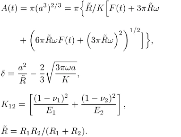
The tip/nanoparticle and nanoparticle/substrate inter-actions induce deformation on the contact surfaces. To model the contact elastic deformation, we use JKR contact mechanics [22-24]. JKR continuum contact me-chanics includes eects of surface interactions between two contacting solid objects. The contact region radius, a, the contact area, A, and the penetration depth, , between the tip and the particle and also the particle and the substrate are given by:
A(t) = (a3)2=3= nR=K~ hF (t) + 3 ~R!
+
6 ~R!F (t) +3 ~R!2 1=2io
; = a~2
R 2 3
r 3!a
K ; K12=
(1 1)2
E1 +
(1 2)2
E2
; ~
R = R1R2=(R1+ R2): (18)
In the above equations, F (t) is the normal force in the contact area. ! is the work of adhesion and for the two contact surfaces is obtained as [25]:
where is the surface energy. ~R is the equivalent radius of the two contact surfaces, K is the equivalent elastic modulus of the two contact surfaces, and and E are Poisson ratio and Young's modulus.
2.5. Dynamic nano friction force
Unlike macroscopic friction, nano friction is velocity dependent, and stick-slip behavior is a major char-acteristic of nano friction [26,27]. Researchers have proposed the LuGre friction model to describe the observed phenomena in nanoscale [28,29]. The Lu-Gre friction model exhibits a truly dynamical model which has been strongly analyzed and contains mathe-matical properties such as the existence and unique-ness of a solution and the boundedunique-ness of a solu-tion [30].
The bristle deection is presented as the state of the friction model. The bristle can be conceived as a cantilever rigidly connected to a body that deects and slips through a terrain as the body is dragged across a surface. Figure 4 illustrates the schematic of the LuGre friction model.
In addition to having mentioned mathematical properties, the LuGre friction model also facilitates appropriate parameter tuning to obtain the friction response, as shown in Figure 5. In addition to slick-slip responses, a dependency on sliding velocity is another characteristic of the LuGre nano friction model.
The LuGre friction model will be used in this paper to characterize nano friction interaction between the nanoparticle and the substrate as follows [30,31]:
Figure 4. LuGre friction model [31].
Figure 5. LuGre friction model response [31].
Ffrict= 0bp(t) + 1( _yp(t))dbdtp(t)+ F_yp(t);
dbp
dt = _yp j _ypj
g( _yp)bp;
g( _yp) =1 0
h
Fc+ (Fs Fc)e ( _yp=s)2
i ;
1( _yp) = 1e ( _yp=d)2; (19)
where bp(t) is bristle deection, _yp(t) is the
nanoparti-cle velocity along the manipulation direction, Fsand Fc
are the static and kinetic friction magnitudes, respec-tively, 0 is bristle stiness, 1 is the bristle damping
coecient, F is the viscous damping coecient, s
is the Stribeck velocity constant and d is a velocity
constant.
3. Controller design
This section is devoted to the design of an optimal sliding mode-based controller. The purpose of the controller is to maintain the tip at a constant height above the sample surface while the probe stage moves laterally, and the tip manipulates the target nanopar-ticle by exerting direct pushing force. The control scheme is illustrated in Figure 6.
3.1. Optimal sliding mode approach
Sliding mode control theory provides some essential tools to control systems with uncertainties or noise. The main problem with this method is that large amounts of control signal may be generated, which leads to control saturation or high energy expenditure. Consequently, optimizing this method may be useful.
Designing an optimal sliding surface for a time-invariant system has been studied by many researchers. In 1996, Koronodi et al. [4] designed an optimal
Figure 6. Control scheme for positioning the cantilever tip at a constant height above the sample substrate during lateral nanomanipulation.
sliding mode controller using the LQ method for a linear time invariant system. Tang and Misawa [32] used the LQR technique for sliding surface design. A linear sliding surface was utilized by both these papers. The designed optimal sliding surface in these references has two main characteristics: Firstly, it passes through the origin of phase space. Secondly, the slope of the surface is designed to optimize a desired cost function. Transforming this system to a regular form will divide the system into two separate parts; the control law appears explicitly in the rst part, but not in the second part. So, the second part is an uncontrolled part and is known as the internal dynamics of a system. The slope of the sliding surface is designed based on internal dynamics, inasmuch as the stability of the overall system will be established by this part.
The transformation matrix, which transforms a system to an appropriate form such as a regular form, does not exist for all nonlinear systems. Hence, the choice of an optimal sliding surface is more complicated in nonlinear systems. Thus far, many methods have been developed to choose an optimal sliding surface for a nonlinear function. Zhou et al. [33] designed an optimal sliding-mode controller for guiding a homing missile to a maneuvering target. They considered target maneuvers as a system disturbance. So, sliding mode control provides them with a robust control strategy to reliably reach the target. In 2006, Nikkhah and Ashrauon [34] developed a method for optimal control of under-actuated systems. Bahrami et al. [35] also designed an optimal sliding mode controller for an aerospace application. Their main goal was to provide robustness against disturbances and increase terminal accuracy. In 2000, Salamci and Ozgoren [36] designed an optimal sliding mode controller for a missile autopilot by approximating the nonlinear system as a linear system.
In this study, the results of [36] are used to design optimal sliding surfaces for the main nonlinear system (Eqs. (7) to (9) and (14)). First, a linearization of the nonlinear system about an operating point, via the Taylor's series expansion method, is used to design the slope of the sliding surface. The linearized model does not obviously represent the global behavior of the original nonlinear system. Hence, the sliding controller which is modeled based on a linearized system, is suitable for a close neighborhood of the operating point. So, utilizing successive linearized models at operating points can extend the operating region of a sliding controller. Finally, control inputs which result from the linearized model are exerted to the nonlinear system [37,38].
3.2. Optimal sliding mode controller design approach
The nonlinear system of concern is represented by:
d
dtx = A(x)x + B(x)u; x 2 Rn; u 2 Rm;(20) where, n = 8 is the number of state variables and m = 1 is the number of control inputs. The states are , yt, yp, ztand their derivatives. To design an optimal
sliding surface, the system should be approximated as a sequence of linear time varying systems. For this purpose, it is linearized via the Taylor's series expansion method about each operating point, as follows [4,36]:
d
dtx = A(t)x + B(t)u; x 2 Rn; u 2 Rm:(21) This equation can be converted to the following form:
d dt x1 x2 =
A11 A12
A21 A22
x1 x2 + 0 B2 u; (22)
where x12 Rn m, x22 Rm. The sliding surfaces can
be written as:
s = x2+ KLQx1 s 2 Rm; (23)
in which KLQ should be specied as a design
parame-ter. Indeed, dierent amounts of KLQ cause dierent
performances. In this work, the LQ method is used to determine KLQ [4].
So, consider the subsystem: d
dtx1= A11x1+ A12x2; (24) and the motion on the LQ optimal sliding surface minimizes the following cost function [6]:
J = 12 Z t
0 fx1(t) TQ
1x1(t) + x2(t)TR1x2(t)gdt: (25)
So, the KLQwill be calculated from:
KLQ= R11AT12P; (26)
in which P > 0 is the solution of the following Riccati equation:
P A11+ AT11P P A12R11AT12P + Q1+ 0: (27)
Now, to determine ueq, _s should be equal to zero.
_s = _x2+ KLQ_x1= 0: (28)
Control signal ui (i = 1 : : : m) equals:
ui= uieq+ Misat
si
'
; (29)
where Mi and ' are constant parameters. Using the
Lyapunov function, V =1
2sTs, we must be sure that:
si_si< 0: (30)
In the following section, the proposed approach is applied to the nonlinear dynamics of the AFM. In this work, it is assumed that there is no uncertain parameter in the model.
4. Simulation results and discussion
Simulation of the nanomanipulation process after im-plementation of the designed controller is performed. The simulations include the manipulation of a gold-coated particle on a silicon oxide substrate by an
AFM tip made of silicon. The chosen materials are widely used in experiments, so comparison can be made easily. The values of system parameters are listed in Table 1 [5,10,19,39,40].
For a nanomanipulation task, the AFM probe stage moves with a constant lateral velocity (Vstage)
Table 1. System parameters values for simulation [5,10,19].
Symbol Quantity Value
Geometry and mechanical parameters
T Microcantilever beam thickness 1 10 6 m
W Microcantilever beam width 48 10 6 m
L Microcantilever beam length 225 10 6m
Microcantilever beam density 2330 kg/m3
E Microcantilever beam Young's modulus 169 109 Pa
Microcantilever beam Poisson's ratio 0.27
H AFM tip height 12 10 6 m
mt AFM tip mass 3 10 10kg
It AFM tip moment of inertia 23:4 10 22 kg.m2
Rt AFM Tip apex radius 25 10 9 m
Rp Particle radius 150 10 9m
p Particle density 2230 kg/m3
t Tip Poisson ratio 0.17
P Particle Poisson ratio 0.42
S Substrate Poisson ratio 0.16
Et Tip Young's modulus 135 109 Pa
EP Particle Young's modulus 3:8 109 Pa
ES Substrate Young's modulus 73 109 Pa
Adhesion parameters
t Tip surface energy 1.4 J/m2
p Particle surface energy 1.5 J/m2
s Substrate surface energy 0.16 J/m2
a0 Interatomic separation distance 3:75 10 10 m
Htp Hamacker constant (Si-Water-Au) [39] 33:6 10 20 J
Hps Hamacker constant (Au-Water-SiO2) [40] 8:1 10 20J
Friction parameters
FS Static friction magnitudes 1 10 9 N
FC Kinetic friction magnitudes 6 10 10N
0 Bristle stiness 1 105 N/m
1 Bristle damping coecient 1:5 10 6N.s/m
s Stribeck velocity constant 1 10 5 m/s
d Velocity constant 0.1 m/s
F Viscous damping coecient 0 N.s/m
Simulation parameters
Vstage Stage velocity 5 10 5 m/s
hset Desired tip center height 7:68 10 8 m
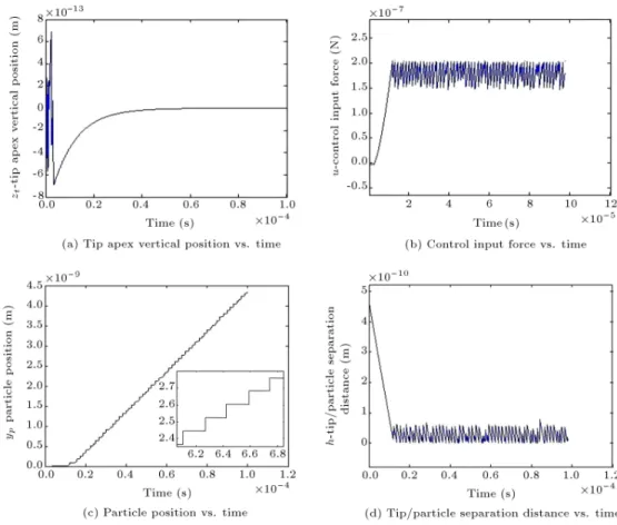
Figure 7. Simulation results of nanoparticle manipulation by an AFM tip controlled using optimal sliding mode.
and approaches the target nanoparticle while the AFM tip is controlled to track a specied trajectory. The particle is supposed stationary on the substrate from the beginning. The separation distance between the tip-particle decreases gradually until the tip apex reaches the contact region with the particle and, then, the attractive interaction force between the tip-particle converts to a repulsive force. Due to the repulsive interaction force, the lateral deection and torsional angle of the AFM tip increases, while the tip vertical position is controlled in order to remain at the horizontal line. Whenever the repulsive pushing force overcomes the LuGre friction force between the particle-substrate, the particle starts sliding on the substrate. It ceases again when the friction force becomes larger than the pushing force. The LuGre friction force is a function of the particle velocity and increases rapidly after particle movement. This stick-slip response repeats during the nanomanipulation task. Simulation of the nanoparticle manipulation is performed, while the controller is employed to control the AFM tip height. The simulation results have been shown over a short time for a better illustration of the parameters responses and behaviors. Nevertheless, the simulation results for a much longer simulation time showed the same bounded responses, as long as we keep the dened experiment conditions and simulation parameters constant.
Figure 7(a) depicts the tip apex vertical position versus time. As shown, the proposed controller main-tains the tip apex on the desired trajectory, which is chosen as a horizontal line. The tracking simulation response shows that the tip has a slight undershoot and then returns to the desired line with an acceptable resolution. The input force signal is depicted in Figure 7(b), and it is shown to be bounded. It initially jumps to an approximately constant value, and uctuates about this value when the system reaches a steady-state behavior and the tip-particle remains in the contact mode.
The particle position versus time is depicted in Figure 7(c). Initially, the nanoparticle stays motionless and then moves with a stick-slip behavior on the sub-strate in the y-axis direction, as shown in Figure 7(c). This gure indicates that the particle periodically ex-periences a positive and negative acceleration. During the particle stick-slip motion, the particle has positive acceleration while the pushing force is dominant over the friction force, and it has negative acceleration when the friction force becomes larger. The average velocity of the nanoparticle is about 0.5 m/s, which is equal to the velocity of the probe stage.
Figure 7(d) shows the separation distance be-tween the external surfaces of the particle-tip after nanoscale deformation. As shown, the parameter decreases until it reaches the contact region, according
to the Derjaguin interaction model, and after that, the nanoparticle starts to move. This parameter uctuates around a constant value of about 21 Angstrom. During the particle stick-slip motion, the separation distance increases while the particle slides on the substrate and decreases when the particle is in the sticking phase.
By solving the Riccati equation for P > 0, optimal sliding mode coecients (KLQi(i = 1 7)) can be
calculated from Eq. (25), as shown in Figure 8(a)-(d). These gures show that the slopes of the optimal sliding surface are tuned after a while, and then, they reach a smaller and constant value. Table 2 shows their nal values. Figure 8(b) and (c) show that K3, K4and K5
are larger than other coecients. These coecients correspond to the yp, zt and _ states. Consequently,
Table 2. Final values of KLQ.
Final values
K1 K2 K3 K4 K5 K6 K7
540.3 340.3 9302 8271.8 12030.1 12.3 0.03
they are the chief states in the optimal sliding mode controller design.
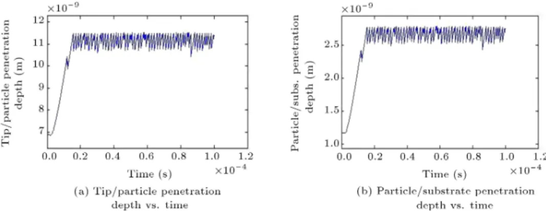
Contact deformations between the tip-particle and the particle-substrate are obtained using a JKR contact mechanics model, and are depicted in Figure 9. The tip-particle penetration depth is presented in Figure 9(a). The graph has an initial jump, which corresponds to the tip-particle approaching time, and when the tip approaches and remains in the contact region with the particle, the graph shows a stick-slip pattern. The particle-substrate penetration depth on the contact surface is also given in Figure 9(b). The prole similarly shows an initial jumping and follows a stick-slip pattern with increasing and decreasing amplitude, with respect to time.
5. Conclusion
An optimal sliding mode approach is applied to the AFM probe in order to control and suppress the
Figure 8. Optimal sliding mode coecients over time (KLQi(i = 1 7)).
vibration behavior of the AFM microcantilever for a 2-D lateral nanomanipulation task. In this paper, a complete model of the pushing based manipulation of a nanoparticle by an AFM probe is presented. The proposed nanomanipulation model is divided into the AFM probe and the nanoparticle dynamics, and consists of all eective phenomena in the nanoscale. Nanoscale interaction forces, elastic deformation in contact areas, and dynamic friction force are considered in the tip-particle-substrate system model. The pro-posed dynamic friction model depends on the relative velocity and produces the stick-slip behavior of the nanoparticle.
The optimal sliding mode control approach pro-vided good performance with a simple control struc-ture. In this control approach, slope tuning of the sliding surface is chosen using the LQ method in order to optimize the cost function. First, a successive approximation approach is used to approximate the main nonlinear system as a linear time variant system at each operating point. Then, the LQ method is used to design the control input for approximated systems. The control input which is generated from the approximated system is applied to the original nonlinear system. The simulation results showed that the proposed controller law can track the desired trajectory with perfect accuracy.
References
1. Delnavaz, A., Jalili, N. and Zohoor, H. \Vibration control of AFM tip for nano-manipulation using com-bined sliding mode approach", 7th IEEE Int. Conf. on Nanotechnology, Hong Kong, China, pp. 106-111 (2007).
2. Sitti, M. and Hashimoto, H. \Controlled push-ing of nanoparticles: Modelpush-ing and experiments", IEEE/ASME Trans. on Mechatron., 5(2), pp. 199-211 (2000).
3. El Rai, K., El Rai, O. and Toumi, K.Y. \Modeling and control of AFM-based nano-manipulation sys-tems", IEEE Int. Conf. on Robotics and Automation, Barcelona, Spain, pp. 157-162 (2005).
4. Koronodi, P., Hashimoto, H., Gajdar, T. and Suto, Z. \Optimal sliding mode design for motion control", IEEE Int. Symp. on Industrial Electronics, Warsaw, Poland, 1, pp. 277-282 (1996).
5. Tafazzoli, A. and Sitti, M. \Dynamic behavior and simulation of nanoparticle, sliding during nanoprobe-based positioning", IMECE/ASME Int. Mechanical Eng. Congress & Exposition, Anaheim, CA, pp. 965-972 (2004).
6. Tafazzoli, A., Pawashe, C. and Sitti, M. \Atomic force microscope based two-dimensional assembly of micro/nanoparticles", IEEE Conf. on Nanotechnology, Montreal, Canada, pp. 230-235 (2005).
7. Tafazzoli, A. and Sitti, M. \Dynamic modes of nano-particle motion during nanoprobe based manipula-tion", IEEE Conference on Nanotechnology, Munich, Germany (2004).
8. Korayem, M.H. and Zakeri, M. \Sensitivity analysis of nanoparticles pushing critical conditions in 2-D controlled nanomanipulation based on AFM", Int. J. Manuf. Tech., 41, pp. 714-726 (2008).
9. Zhou, Q., Kallio, P., Aria, F., Fukuda, T. and Koivo, K.N. \A model for operating spherical micro objects", 10th Int. Symp. on Micro-mechatronics and Human Science, Nagoya-shi, Japan, pp. 79-85 (1999).
10. Mualim, Y., Ghorbel, F. and Dabney, J.B. \AFM nano-manipulation modeling and simulation", IMECE/ASME Int. Mechanical Eng. Congress & Ex-position, Chicago, IL, USA (2006).
11. Landolsi, F., Ghorbel, F.H. and Dabney, J.B. \An AFM-based nanomanipulation model describ-ing the atomic two dimensional stick-slip behavior", IMECE/ASME Int. Mechanical Eng. Congress & Ex-position, Seattle, WA, USA, pp. 177-186 (2007). 12. Mahboobi, S.H., Meghdari, A., Jalili, N. and Amiri,
F. \Two-dimensional atomistic simulation of metallic nanoparticles pushing", Mod. Phys. Lett. B, 23(22), pp. 2695-2702 (2008).
13. Mahboobi, S.H., Meghdari, A., Jalili, N. and Amiri, F. \Qualitative study of nanocluster positioning process: Planar molecular dynamics simulations", Curr. Appl. Phy., 9(5), pp. 997-1004 (2009).
14. Jalili, N., Dadfarnia, M. and Dawson, D.M. \A fresh insight into the microcantilever-sample interac-tion problem in non-contact atomic force microscopy", ASME J Dyn. Syst., Meas., Control, 126(2), pp. 327-335 (2004).
15. Ashhab, M., Salapaka, M.V., Dahleh, M. and Mezic, I. \Dynamic analysis and control of microcantilevers", Automatica, 35(10), pp. 1663-1670 (1999).
16. Sitti, M. and Hashimoto, H. \Macro to nano tele-manipulation through nanoelectromechanical sys-tems", 24th IEEE Industrial Electronics Society An-nual Conf., Aachen, Germany, 1, pp. 98-103 (1998). 17. Saeidpourazar, R. and Jalili, N. \Towards fused vision
and force robust feedback control of nanorobotic-based manipulation and grasping", Mechatronics, 18(10), pp. 566-577 (2008).
18. Stark, R.W., Schitter, G. and Stemmer, A. \Tuning the interaction forces in tapping mode atomic force microscopy", Physical Review B, 68, 085401 (2003). 19. Sitti, M. \Atomic force microscope probe based
con-trolled pushing for nanotribological characterization", IEEE/ASME Transactions on Mechatronics, 9(2), pp. 343-349 (2004).
20. Tian, X., Wang, Y., Xi, N. and Dong, Z. \A study on theoretical nano forces in AFM based nanomanipula-tion", 2nd IEEE Int. Conf. on Nano/Micro Engineered and Molecular Systems, Bangkok, Thailand, pp. 917-921 (2007).
21. Yang, Q. and Jagannathan, S. \Nanomanipulation using atomic force microscope with drift compensa-tion", IEEE American Control Conf., Minneapolis, MN, USA, pp. 514-519 (2006).
22. Bhushan, B., Introduction to Tribology, John Wiley and Sons, New York (2002).
23. Israelachili, J., Intermolecular and Surface Forces, 2nd Ed., Academic Press London (1992).
24. Johnson, K.L., Contact Mechanics, Cambridge Univer-sity, London (1985).
25. Jalili, N., Dadfarnia, M. and Dawson, D.M. \A fresh insight into the microcantilever-sample interac-tion problem in non-contact atomic force microscopy", ASME J. Dynamic Syst. Meas. Control, 126, pp. 327-35 (2004).
26. Falvo, M.R., Taylor, R.M., Helser, A., Chi, V., Brooks, F.P., Washburn, S. and Superne, R. \Nanometer-scale rolling and sliding of carbon nanotubes", Nature, 397, pp. 236-238 (1999).
27. Braiman, Y., Family, F. and Hentschel, H.G.E. \Non-linear friction in the periodic stick-slip motion of coupled oscillators", Phys. Rev. B, 55, pp. 5491-5504 (1997).
28. Meurk, A. \Microscopic stick-slip in friction force microscopy", Tribol. Lett., 8, pp. 161-169 (2000). 29. Stark, R.W., Schitter, G. and Stemmer, A.
\Veloc-ity dependent friction laws in contact mode atomic force microscopy", Ultramicroscopy, 100, pp. 309-317 (2004).
30. Olsson, H. \Control systems with friction", Disserta-tion, Lund Institute of Technology (1996).
31. Mualim, Y. \Nanomanipulation modeling and simula-tion", Master's Thesis, Rice University (2007). 32. Tang, C.Y. and Misawa, E.A. \Sliding surface design
for discrete VSS using LQR technique with a present real eigenvalues", IEEE American Control Conference, San Diego, CA, USA (1999).
33. Zhou, D., Chundi, M., Ling, Q. and Xu, W. \Optimal sliding mode guidance of homing missile", 38th IEEE Conf. on Decision and Control, Phoenix, AZ, USA, 5, pp. 5131-5136 (1999).
34. Nikkhah, M. and Ashraun, H. \Optimal sliding mode control for underactuated systems", IEEE American Control Conf., Minneapolis, MN, USA (2006). 35. Bahrami, M., Ebrahimi, B. and Roshanian, J.
\Op-timal sliding-mode guidance law for xed interval propulsive maneuvers", IEEE Int. Conf. on Control Applications, Munich, Germany, pp. 1014-1018 (2006). 36. Salamci, M.U. and Ozgoren, M.K. \Sliding mode con-trol with optimal sliding surfaces for missile autopilot design", J. Guid. Control Dyn., 23(4), pp. 719-727 (2000).
37. Yeh, F.K., Chein, H.S. and Chen, L. \Design of optimal midcourse guidance sliding-mode control for missiles with TVC", IEEE Transactions on Aerospace and Electronic Systems, 39(3), pp. 824-837 (2003).
38. Novin Zade, A. \Closed loop optima-fuzzy control in nonlinear systems", Dissertation, Sharif University of Technology (2005).
39. Rollot, Y., Regnier, S. and Guinot, J.C. \Simulation of micro-manipulation: Adhesion forces and specic dynamic models", Int. J. Adh. & Adh., 19, pp. 35-48 (1999).
40. De Wit, C., Olsson, H., Astrom, K.J. and Lischinsky P. \A new model for control of systems with friction", IEEE Trans. Automatic Control, 40(3), pp. 419-25 (1995).
Biographies
Hesam Babahosseini received his BS degree from the International University of Imam Khomeini, Qazvin, Iran, in 2007, and his MS degree from Sharif University of Technology, Tehran, Iran, in 2010, both in Mechan-ical Engineering. He is currently working towards a PhD degree in Mechanical Engineering in the Virginia Tech Microelectromechanical Systems Laboratory at the Bradley Department of Electrical and Computer Engineering, Virginia Polytechnic Institute and State University, Blacksburg, USA.
His research interests include bioMEMS, microu-idics, micro-fabrication, and AFM with applications in cellular biomechanics and mechanobiology investi-gations.
Seyed Hanif Mahboobi received his BS, MS and PhD degrees in Mechanical Engineering, in 2002, 2004 and 2009, respectively, from Sharif University of Technology, where he was also a member of the Center of Excellence in Design, Robotics, and Au-tomation (CEDRA). He then attended the Institute for Nanoscience and Nanotechnology (INST) as a postdoctoral researcher. He is currently a postdoctoral researcher at the California Institute for Quantitative Biosciences at UC Berkeley, USA. His research in-terests include robotics, nanomanipulation, computa-tional nanoscience and biomolecular simulation. Majid Khorsand Vakilzadeh received his BS and MS degrees in Mechanical Engineering from Amirk-abir University and Sharif University of Technology, respectively, and is currently pursuing his PhD degree in the Department of Applied Mechanics at Chalmers University of Technology, Sweden. His research is focused on structural dynamics, model order reduction and stochastic nite element model updating.
Aria Alasty received his BS and MS degrees in Mechanical Engineering from Sharif University of Tech-nology (SUT), Tehran, Iran, in 1987 and 1989, respec-tively, and a PhD degree in from Carleton University, Ottawa, Canada, in the same subject, in 1996. He is
currently Professor of Mechanical Engineering in Sharif University of Technology, and has been a member of the Center of Excellence in Design, Robotics, and Au-tomation (CEDRA) since 2001. His elds of research are mainly in nonlinear and chaotic systems control, computational nano/micro mechanics and control, spe-cial purpose robotics, robotic swarm control, and fuzzy system control.
Ali Meghdari received his PhD degree in Mechanical Engineering from the University of New Mexico in 1987, and then collaborated with the robotics group of the Los Alamos National Laboratory (LANL) as a postdoctoral research fellow. From 1996-1999 he chaired the School of Mechanical Engineering at Sharif University of Technology, Tehran, Iran. From 2001-2010, he also served as Provost and Vice-President of Academic Aairs at the university and is currently Director of the Center of Excellence in Design, Robotics and Automation (CEDRA), and in 1997 was granted the rank of professor, and was recognized by the
Iranian Society of Mechanical Engineers (ISME) as the youngest (at age 37) ME full-professor in Iran. During 1993-94, he was a visiting research faculty at the AHMCT center of the University of California-Davis, and from 1999-2000, he served the IBDMS and RMMRL research centers of the Colorado School of Mines as a visiting research professor.
Dr. Meghdari has performed extensive research in the areas of robotics kinematics/dynamics, nano-manipulations and modeling of biomechanical systems. He has published over 220 technical papers in refereed international journals and conferences, and supervised numerous MS and PhD dissertations. He has also been the recipient of various scholarships and awards. He is on the editorial board of various engineering journals, and an aliate member of the Iranian Academy of Sciences (IAS), the latest being: the 2012 Allameh Tabatabee Distinguished Professorship Award for Ex-cellence in Teaching and Research by the National Elite Foundation of Iran. He is a fellow of the ASME (American Society of Mechanical Engineers).

![Table 1. System parameters values for simulation [5,10,19].](https://thumb-us.123doks.com/thumbv2/123dok_us/8392602.2229860/7.892.199.715.302.1158/table-system-parameters-values-for-simulation.webp)