Didion_unc_0153D_14419.pdf

GENETIC ANALYSIS OF MEIOTIC DRIVE SYSTEMS IN THE MOUSE USING GENOTYPING ARRAYS

John P. Didion

A dissertation submitted to the faculty of the University of North Carolina at Chapel Hill in partial fulfillment of the requirements for the degree of Doctor of Philosophy in the Curricu-lum in Bioinformatics and Computational Biology.

Chapel Hill 2014

Approved by:

Fernando Pardo-Manuel de Villena

c

2014

ABSTRACT

John P. Didion: Genetic Analysis of Meiotic Drive Systems in the Mouse Using Genotyping Arrays.

(Under the direction of Fernando Pardo-Manuel de Villena.)

ACKNOWLEDGMENTS

This research was only possible because of the support given by my mentors, collabo-rators, lab members and funding sources. There have been many over the years who have contributed in ways large and small. If I have forgotten anyone, it is due to lack of memory rather than appreciation.

First and foremost, I am grateful to my advisor, Fernando Pardo-Manuel de Villena. He has been instrumental in my development as a scientist and in providing the vision for my research.

I have been very fortunate to work with many excellent post-docs, students and staff in the lab: David Aylor, John Calaway, Andrew Morgan, Leeanna Hyacinth, Tim Bell, Darla Miller, Ryan Buus, Justin Gooch, Mark Calaway, Ginger Shaw, Nicole Miller, Sara Cates, Teresa Mascenik, Stephanie Hansen and Jennifer Shockley.

I am grateful to have had funding support throughout my graduate career from the follow-ing organizations: Bioinformatics and Computational Biology Trainfollow-ing Grant, the Center for Genome Dynamics, and the Center for Integrated Systems Genomics.

I would like to thank the members of my thesis committee for encouragement and fruitful discussions: Shawn Gomez (Chair), Terry Furey, Jason Leib, Gary Churchill and Jeremy Searle.

TABLE OF CONTENTS

LIST OF TABLES . . . xi

LIST OF FIGURES . . . xii

LIST OF ABBREVIATIONS . . . xv

1 BACKGROUND AND INTRODUCTION . . . 1

1.1 Meiosis and meiotic drive . . . 1

1.2 Requirements for meiotic drive . . . 4

1.3 Types and examples of meiotic drive systems . . . 6

1.3.1 Drive at MI: centromeric drive . . . 6

1.3.2 Drive at MII . . . 9

1.3.3 Modifiers of meiotic drive . . . 11

1.4 Genetic characterization of meiotic drive in the mouse . . . 12

2 DESIGN AND USE OF GENOTYPING ARRAYS FOR GENETIC ANALYSIS OF WILD AND INBRED MICE . . . 14

2.1 The house mouse,Mus musculus . . . 14

2.2 SNP genotyping arrays . . . 17

2.3 The Mouse Diversity Array . . . 18

2.4 Ascertainment bias . . . 19

2.5 Variable intensity oligonucleotides (VINOs) . . . 20

2.6 Diagnostic SNPs . . . 29

2.8 Subspecific origin of laboratory mice . . . 31

2.9 Haplotype and sequence diversity . . . 34

2.10 The MegaMUGA genotyping array . . . 37

2.11 Studies using the MegaMUGA array . . . 39

2.12 Future work . . . 42

3 GENETIC DETERMINANTS OF MEIOTIC DRIVE IN CHROMOSOMAL RACES OF THE HOUSE MOUSE . . . 44

3.1 The chromosomal races ofM. m. domesticus . . . 44

3.2 Introduction to the study . . . 50

3.3 GWAS design . . . 52

3.4 Results . . . 53

3.4.1 The Wild Mouse Genetic Survey is a rich resource for mouse genetics 53 3.4.2 Substantial population structure exists inM. musculusmice genotyped on MDA . . . 55

3.4.3 Heterozygosity varies widely inM. m. domesticuspopulations . . . . 60

3.4.4 Linkage disequilibrium decays rapidly in wild mice . . . 62

3.4.5 First-stage GWAS identifies a significant association between geno-type and 2N . . . 66

3.4.6 Pericentric regions have reduced genetic variation in CRs . . . 71

3.4.7 Chromosomal races are enriched for loci under positive selection . . . 74

3.5 Discussion . . . 75

3.5.1 Are wild mice suitable for association studies? . . . 75

3.5.2 Genetic variants associated with Rb fixation . . . 78

3.5.3 What mechanisms may enable the fixation of metacentric karyotypes? 79 3.5.4 The centromeric drive model of chromosomal race evolution . . . 81

3.6.1 Genotyping . . . 84

3.7 Future Directions . . . 85

3.7.1 Stage-two GWAS . . . 85

3.7.2 Characterization of candidate loci . . . 86

3.7.3 Sequence analysis of wild mice . . . 87

4 GENETIC CHARACTERIZATION OF A NOVEL MEIOTIC DRIVE SYSTEM IN THE MOUSE . . . 91

4.1 Genetic Reference Populations . . . 91

4.2 The Collaborative Cross . . . 92

4.3 The Diversity Outbred . . . 94

4.4 Introduction to the study . . . 94

4.5 Results . . . 97

4.5.1 Extreme TRD in Chr 2 is present in the DO population . . . 97

4.5.2 TRD is exclusive to heterozygous females . . . 98

4.5.3 R2d2maps to a 9.3 Mb interval in the middle of mouse Chr 2 . . . 101

4.5.4 A 4.3 Mb-long expansion is the causative allele atR2d2. . . 103

4.5.5 Meiotic drive causes maternal TRD atR2d2 . . . 107

4.6 Discussion . . . 110

4.6.1 How do meiotic drive and embryonic lethality contribute to TRD at R2d2? . . . 110

4.6.2 Mapping the responder and identification of the causative allele . . . 111

4.6.3 Is meiotic drive atR2d2a polygenic trait? . . . 115

4.6.4 What is the mechanism by whichR2d2influences segregation incis . 116 4.6.5 Revisiting TRD in the CC and DO . . . 118

4.6.6 Evolutionary origin ofR2d2 . . . 122

4.7.1 Ethics statement . . . 123

4.7.2 Published mouse crosses . . . 124

4.7.3 New mouse crosses . . . 124

4.7.4 DNA isolation and genotyping . . . 125

4.7.5 CC and DO haplotypes . . . 125

4.7.6 Estimation of embryonic lethality . . . 126

4.7.7 Statistics . . . 126

4.7.8 Linkage mapping of theR2d2expansion . . . 127

4.7.9 Fine-mapping of theR2d2expansion . . . 128

4.7.10 Sequence variants and read depth . . . 129

4.8 Future directions . . . 130

4.8.1 Molecular characterization ofR2d2and modifier loci . . . 130

4.8.2 Genetic characterization ofR2d2in natural populations . . . 130

5 CONCLUSIONS . . . 133

5.1 Implications of meiotic drive . . . 134

5.1.1 Changes in population allele frequencies . . . 134

5.1.2 Changes in centromere size and sequence . . . 135

5.1.3 Changes in chromosome size and organization . . . 135

5.1.4 Karyotype evolution and speciation . . . 136

5.1.5 Human population genetics and health . . . 140

5.2 Contributions of my studies . . . 141

5.2.1 The Wild Mouse Genetic Survey (WMGS) . . . 141

5.2.2 Characterization of meiotic drive using genotyping arrays . . . 142

5.2.3 Genetic control of meiotic drive . . . 142

5.3 Future applications of our work . . . 145

5.3.1 Genetic control of invasive mouse populations . . . 146

6 APPENDIX A: GENOTYPING ARRAY METHODS . . . 150

A-1 DNA isolation and array processing . . . 150

A-2 Normalization . . . 150

A-3 Clustering and genotyping . . . 151

A-4 Quality control . . . 152

A-5 Copy number analysis . . . 153

A-5.1 Sex determination . . . 153

A-6 Phasing and imputation . . . 154

A-7 Relatedness . . . 155

A-8 Tree reconstruction . . . 156

LIST OF TABLES

3.1 Chromosomal Races ofM. m. domesticus . . . 46

4.1 Segregation ratios in the progeny ofR2d2WSB/otherheterozygous F1 hybrid sires and dams . . . 100 4.2 Segregation ratios in the progeny ofR2d2WSB/other_{heterozygous F1 hybrid sires}

LIST OF FIGURES

1.1 Simplified schematic of a mammalian meiosis . . . 3

1.2 Requirements for meiotic drive . . . 5

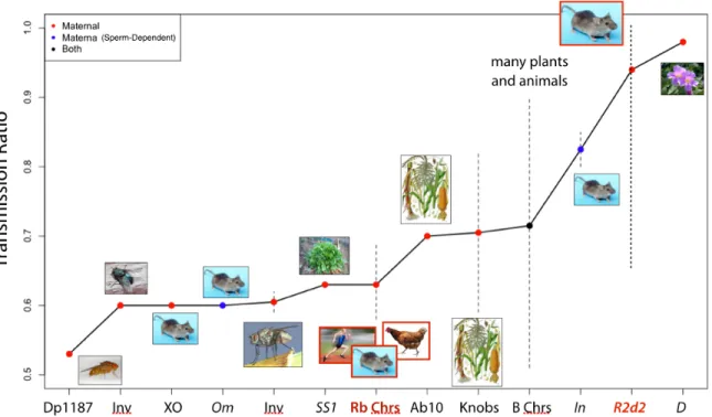
1.3 Summary of meiotic drive systems in plant and animal species . . . 7

2.1 The phylogeny ofM. musculus . . . 15

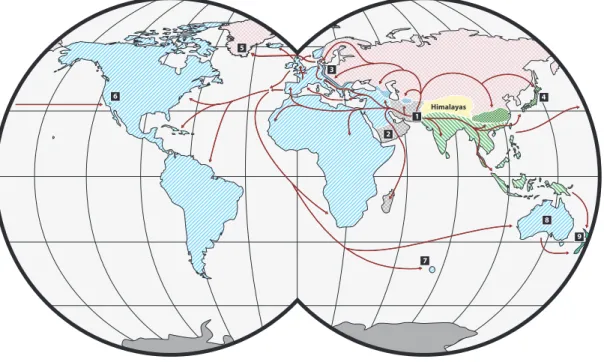
2.2 Origin and historical migrations ofM. musculussubspecies . . . 16

2.3 VINOs are identified as a cluster of low-intensity samples . . . 21

2.4 Non-homozygous VINO call rates increase with divergence from the reference genome . . . 24

2.5 OTV position in the probe and RFLP have significant effects on hybridization intensity and VINO detection . . . 26

2.6 Detected and undetected VINOs in homozygosity may lead to inaccurate geno-typing in heterozygosity . . . 27

2.7 The distance between consecutive SNPs follows a geometric distribution . . . 28

2.8 VINOs improve the topology of phylogenetic trees . . . 31

2.9 The phylogeny of wild-derived strains . . . 35

2.10 Nucleotide diversity is greater in wild mice than classical strains . . . 37

2.11 MegaMUGA can identify chromosome loss . . . 42

3.1 Geographic locations of chromosomal races and collected samples . . . 48

3.2 Distribution of Rb fusion pairs is non-random . . . 49

3.3 Design of our two-stage GWAS . . . 53

3.4 MAFs at MDA markers are weighted toward lower values in wild mice . . . . 57

3.5 Principal component analysis of wildM. m. domesticusmice . . . 59

3.7 Inbreeding is variable in wildM. m. domesticusmice . . . 63

3.8 Heterozygosity is variable in CRs . . . 64

3.9 Linkage disequilibrium is minimal in wildM. m. domesticusmice . . . 65

3.10 LD decays rapidly in a sample of unrelatedM. m. domesticusmice . . . 67

3.11 GWAS identifies a significant association on Chr 13 . . . 69

3.12 Haplotype analysis of significant assocation on Chr 13 . . . 70

3.13 Heterozygosity is significantly different between chromosome types . . . 72

3.14 Metacentric chromosomes have reduced MAF in pericentric regions . . . 73

3.15 Enrichment of evidence of selective sweeps in CRs . . . 75

3.16 The majority of metacentrics are of intermediate size . . . 82

3.17 Wild mice selected for whole-genome sequencing . . . 88

4.1 The Collaborative Cross and Diversity Outbred . . . 93

4.2 Chr 2 allele frequencies in the DO . . . 98

4.3 R2d2maps to a 9.3 Mb candidate interval . . . 104

4.4 R2d2is a copy number gain that is novel with respect to the reference sequence 105 4.5 Linkage mapping localizesR2d2to a 900 kb region in Chr 2 . . . 106

4.6 TR and Litter Size are variable in DO and CC crosses. . . 108

4.7 TRD atR2d2is explained by both meiotic drive and embryonic lethality. . . . 109

4.8 QTL mapping of modifiers identifies suggestive associations . . . 117

4.9 Litter sizes are not different between CC lines that fixed WSB/EiJ and non-WSB/EiJ alleles atR2d2 . . . 119

4.10 Fixation ofR2d2WSB _{would occur much faster than predicted . . . 120}

4.11 Selective sweep in the absence of changes in fitness . . . 122

LIST OF ABBREVIATIONS

2N Diploid Number

BAC Bacterial Artificial Chromosome

BF Bayes Factor

CC Collaborative Cross

CNV Copy Number Variant

CR Chromosomal Race

DO Diversity Outbred

GD Gametic Disequilibrium

GRP Genetic Reference Populations

GWAS Genome-Wide Association Study

HMM Hidden Markov Model

HWE Hardy-Weinberg Equilibrium

IBD Identity By Descent

IBS Identity By State

LD Linkage Disequilibrium

MAF Minor Allele Frequency

MDA Mouse Diversity Array

MI Meiosis I

MII Meiosis II

MUGA Mouse Universal Genotyping Array

MYA Million Years Ago

OTV Off-Target Variant

PAR Pseudo-Autosomal Region

PCA Principal Component Analysis

SDP Strain Distribution Pattern

Rb Robertsonian

SNP Single Nucleotide Polymorphism

ST Standard Population

SV Structural Variant

TRD Transmission Ratio Distortion

VINO Variable Intensity Oligonucleotide

Chapter 1

BACKGROUND AND INTRODUCTION

This work examines the phenomenon of meiotic drive in the context of two different sys-tems in the house mouse. The primary aim of these studies is to identify genetic factors that contribute to the presence and variability of non-random chromosomal segregation during fe-male meiosis (meiotic drive). In this chapter, I give an introduction to meiotic drive, followed by an overview of these two studies.

1.1 Meiosis and meiotic drive

Since their rediscovery in the early 20th century, Mendel’s Laws have formed the theo-retical basis for our understanding of the genetics of inheritance. The Law of Segregation (“First Law”) states that alleles at homologous loci segregate from each other during meiotic cell division and are transmitted randomly to gametes. The Law of Independent Assortment (“Second Law”) states that alleles at unlinked loci segregate independently from each other. Together, Mendel’s Laws create one of the strongest predictions in biology: that, for sexu-ally reproducing species, each individual’s genome is a random collection of alleles equsexu-ally derived from its mother and father.

to the Law of Independent Assortment that we now take for granted. Early geneticists also discovered that some genes violated the Law of Segregation [1, 2]. When a violation of the First Law is found to be significant and reproducible, regardless of the cause, it is referred to as transmission ratio distortion (TRD) [3]. Most observations of TRD are due to selection in favor of alleles that increase the fitness of individuals with respect to their environment (ecological selection) or their sexual competitors (sexual selection). Selection may also act upon the products of meiosis (gamete selection) or fertilization (differential embryonic sur-vival). However, an increasing number of observations of TRD can be ascribed to competition between “selfish” genetic elements, which promote their own preferential transmission irre-spective of their effects on individual fitness. This so-called intragenomic conflict has been observed in a wide variety of eukaryotic species [4, 5, 6]. Intragenomic conflict can take many forms, but generally follows one (or more) of three strategies: 1)interference, in which an al-lele prevents the transmission of other alal-leles or prevents the carriers of alternate alal-leles from passing them on; 2)overreplication, in which an allele increases its chances of being transmit-ted by increasing its prevalence in the genome, by duplication or transcriptional upregulation; or 3)gonotaxis, in which an allele moves preferentially into the genetic material that is passed on to subsequent generations [7].

Meiosis is the process by which the germ cells of multicellular, sexually reproducing eu-karyotes give rise to the gamete cells, which in turn fuse during fertilization and transmit the genetic information from parents to their offspring. Although the processes governing meiotic chromosomal segregation are among the most well-conserved features of eukaryotic biology [8], there are examples in many species of genes that selfishly subvert the redundancies and safe-guards. Meiotic drive is a type of intragenomic conflict (specifically gonotaxis) that re-sults in the differential inclusion of parental alleles in the products of meiosis [4].

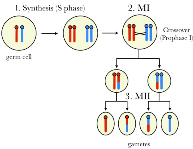
the entire genome is made and each chromosome becomes a complex of two identical sister chromatids; 2) meiosis I (MI), in which each pair of homologous chromosomes is segregated into two haploid daughter cells; and 3) meiosis II (MII), in which each daughter cell divides and the sister chromatids of each chromosome are segregated. An important distinction be-tween MI and MII is that during prophase of MI (prophase I), homologous chromosomes pair (synapsis) and attach to one another at points called chiasmata. When the meiotic spindle pulls the homologous chromosomes apart, some chiasmata are resolved as crossovers that result in the exchange of genetic material between the homologous chromosomes (recombination).

Figure 1.1: Simplified schematic of a mammalian meiosis. Two parental chromosomes (red and blue) are replicated during S phase (1). Homologues crossover at least once per chro-mosome arm during the first meiotic cell division (2). Finally, a second meiotic division (3) results in haploid gamete cells.

cells of roughly equal size. In contrast, each cell division in female meiosis results in one viable product containing the vast majority of the volume of the progenitor cell, and one non-viable “polar body.” Therefore, each female meiosis results in a single gamete (ovum, or egg), while each male meiosis results in four gametes (spermatids). This difference is primarily due to the requirement that the ovum, in addition to carrying the maternal genetic complement, must carry all of the material required for development into a new organism as well as a protective enclosure within which the new organism may develop. Intuitively, it is a better strategy for a female germ cell to put all of its energy into creating a single, robust gamete rather than four smaller viable gametes. However, the asymmetry of female meiosis presents an opportunity for selection: if one allele of a locus that is directly involved in meiotic chromosomal segregation has greater “fitness” than its homologue, it can get into the ovum more than 50% of the time, thereby increasing its frequency. Meiotic drive that results from an allele exploiting asymmetric female meiosis to gain a segregation advantage is called female meiotic drive.

1.2 Requirements for meiotic drive

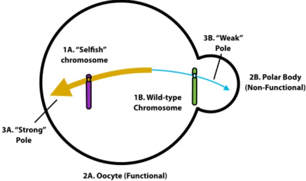
A survey of meiotic drive systems revealed that the necessary and sufficient requirements for drive are only three: 1) meiotic divisions that are asymmetrical with respect to cell fate; 2) functional asymmetry of the meiotic spindle poles; and 3) functional heterozygosity at a locus that mediates attachment of a chromosome to the meiotic spindle [11] (Figure 1.2).

Figure 1.2: Meiotic drive is the non-Mendelian segregation of functionally different chromo-somes (1) that depends on asymmetric female meiosis (2) and the inequality of meiotic spindle poles (3). Adapted from [11].

out during cytokinesis to encapsulate the chromosomes on the externally facing side of the metaphase plate, forming a polar body that degenerates and may be reabsorbed. In contrast to mammalian females, females of some plant and insect taxa undergo two successive meioses without cytokinesis. The meiotic products are arranged linearly, and the innermost product is retained by the oocyte while the remaining three products degenerate.

mice preferentially segregate toward the functional meiotic product. It is speculated that pref-erential segregation of unpaired chromosomes may be due to a meiotic failsafe that, in the presence of an unequal number of centromeres, prefers to retain more genetic material in the oocyte [13].

The third requirement for meiotic drive may be satisfied by a selfish genetic element that, when in heterozygosity, succeeds in being transmitted to the functional product of asymmetric meiosis more than 50% of the time. B chromosomes are only one of several types of loci that exhibit drive.

1.3 Types and examples of meiotic drive systems

Meiotic drive has been reported in several species (Figure 1.3), and has been the subject of much study. The loci at which meiotic drive is observed (responderloci) may be classified by their chromosomal position with respect to the centromere, which determines the phase of meiosis during which drive may occur and also the level of TRD that may be observed. In theory,distorterloci (the loci that induce non-random segregation) may be located anywhere in the genome, although in nearly all meiotic drive systems in which a distorter has been identified it is tightly linked to theresponder.

1.3.1 Drive at MI: centromeric drive

Figure 1.3: Summary of meiotic drive systems in plant and animal species. Colored points indicate the sex specificity of drive: female-only (red), female drive induced by a genetic factor in the fertilizing sperm (blue), and sex-independent. Dotted lines indicate a range of reported transmission ratios. The systems involved in the research presented in Chapters 3 and 4 are highlighted in red.

the functional cell product will increase its frequency in the population (centromeric drive). Centromeric drive must occur at MI since it is only in the primary oocyte that there may be homologous chromosomes with centromeres of different fitness (Figure 1.1). It is thought that centromeric drive may result from an “arms race” between competing centromeric repeat sequences [14].

has been observed in humans [15] and mice (reviewed in [16]) at levels ∼ 60%. Drive is observed independent of which chromosomes are fused. Strikingly, the direction of segre-gation distortion is not consistent: in mice, the acrocentric chromosomes are preferred over the metacentric, while the opposite is true in humans. In both cases, the direction of drive is consistent with the predominant chromosomal form of the species. Conceptually equivalent results are observed in chickens: heterozygous female carriers of chromosome fissions pref-erentially transmit the metacentric∼ 70%of the time [17]. The common feature of meiotic drive involving all of the mentioned chromosomal rearrangements and abnormalities is the unequal number of centromeres on either side of the metaphase plate during meiotic division (the unequal centromere number rule [16]). Therefore, it is most likely that drive is act-ing on the centromeres themselves rather than any particular DNA sequence. It is theorized that drive in favor of either greater or lesser numbers of chromosomes is a common feature across the tree of life. Furthermore, the direction of drive appears to undergo frequent rever-sal over evolutionary time [16], sometimes even within otherwise genetically homogeneous species. This can be observed most dramatically in the extreme karyotype diversity withinM. m. domesticus, discussed in Chapter 3, although intraspecific karyotype variation due to Rb translocations is also known in several other small mammals, e.g., shrews [18]. Meiotic drive of Rb translocations is predicted to contribute to karyotype evolution, especially in species in which Rb translocations are the predominant type of chromosome structural change [19].

female fecundity, meaning that the observed TRD was not due to lethality associated with not having a M. guttatus allele at the D locus. Since the theoretical limit on the maximum distortion that may occur at a non-centromeric locus (∼83%, [21]) is less than the magnitude of drive observed atD, eitherDis the centromere (or tightly linked to the centromere), orD

is driving at both MI and MII. Although an assembly of theMimulusgenome was not avail-able, and thus the physical proximity of theDlocus to the centromere was unknown, a likely

Mimuluscentromeric repeat sequence maps to theDlocus [22]. Furthermore, theDlocus was greatly expanded in size in species exhibiting TRD. There was also low polymorphism near

D, with LD extending up to 2 cM, which strongly suggests thatDis either the centromere or is bounded by structural variants that suppress recombination.

1.3.2 Drive at MII

Centromeres are not the only loci that may drive. In fact, the majority of female drive systems that have been described involve responder loci that are quite distant from a cen-tromere. However, this disparity may be due to the greater difficulty of observing TRD at centromeric vs. non-centromeric loci than to any relative difference in frequency. Systems that involve distalresponderstend to share several features in common. First, theresponders

tend to be located in large heterochromatic regions [23, 24]. In the few cases where the se-quence of these loci has been examined, they appear to consist primarily of tandem repeats that have some homology to centromeric repeat sequences. These large, centromelike re-gions appear to actually function as centromeres during meiosis (neocentromeres). In many cases it has been shown or predicted that structural variants are involved in suppressing re-combination within the loci. Activation of neocentromeres during meiosis may be a specific instance of centromere repositioning, which appears to be frequent in mammals and may play an important role in karyotype evolution [25, 26].

hete-rochromatic sequences (knobs) distinct from the chromosome’s normal centromere. In maize, female meiosis results in the four haploid products extending from the ovary in a row; it is only the basal product (closest to the ovary) that develops into a gamete, while the other three degenerate. The knobs of Ab10 are able to function like centromeres during meiosis and in-teract with the meiotic spindle to greatly increase the chance of the Ab10 homologues being outermost in the ordering of meiotic products, and thus of one of the two being basal. The knobs are active during both male and female meiosis, but it is only in female meiosis that the ordering matters since all of the male meiotic products are viable. The large knob is comprised of a 180bp repeat [28]. There are also three additional supernumerary regions on Chr 10 that function as additional neocentromeres during meiosis and consist of tandem repeats of a dif-ferent, 350bp motif (TR-1). There is evidence of intragenomic conflict between the two types of repeats [29]. Cytogenetic studies have shown that neocentromeres only replicate the ability of true centromeres to move along the meiotic spindle; true centromeres and neocentromeres are otherwise functionally different [30].

10 is the shortest in maize and thus provides the greatest probability of having exactly one recombination between the centromere and large knob [7]. Another consideration is that recombination is undesirable near or within the region containing the genetic elements that are essential for drive. Ab10 contains several structural rearrangements, a large insertion and two nested inversions, that are proposed to suppress recombination in the distal part of the chromosome. All of these facts indicate that chromosomes are subject to natural selection on the position of meiotic drive loci, and that a position at∼50cM leads to chromosomes of the greatest “fitness” in terms of meiosis, even if not in terms of overall organismal fitness.

1.3.3 Modifiers of meiotic drive

meiotic spindle [30].

The only evidence for unlinked modifiers of meiotic drive come from the study of B chro-mosomes in the Mealybug, Pseudococcus afinis. Nur and Brett (1987) [33] found evidence of unlinked loci associated with different rates of B chromosome transmission, however it is not clear whether the distortion was meiotic or post-meiotic. On the other hand, a study of B chromosomes in rye identified modifiers originating from the B chromosomes themselves; however, it was unclear if the modifiers acted in cisonly, or if a modifier on one B chromo-some was able to influence the segregation of other B chromochromo-somes intrans[34].

1.4 Genetic characterization of meiotic drive in the mouse

The house mouse is a good model for expanding our knowledge of the genetic components of meiotic drive. The relatively large number of meiotic drive systems described in the mouse indicate that meiotic drive is at least as frequent in the mouse as in any other species (Figure 1.3). Mice are abundant and relatively easy to capture in the wild, and there are a wealth of re-producible, genetically divergent mouse stocks for laboratory experiments. The mouse is also one of the most popular laboratory model organisms, which has encouraged the development of extensive genetic, cytogenetic, molecular and bioinformatic tools. A significant fraction of my time in the lab has been dedicated to developing technologies and bioinformatic tools to better study natural mouse populations; I discuss these in the next chapter.

My first experimental study (Chapter 3) involved a widely studied set of natural popu-lations. Each of the ∼ 100 chromosomal races (CRs) of the house mouse has a different, non-standard karyotype due to the fixation of one or more metacentric chromosomes that arose by Rb translocation. It has been proposed that meiotic drive is the primary mode of fixation, and that the direction of drive inM. m. domesticus has changed such that metacen-tric chromosomes are selected for, rather than against, during meiosis in females of the CRs. However, there has been no direct evidence of genetic factors that are involved in the change in the direction of drive. The aim of my first investigation was to assemble a large catalogue of genetic variation in wild mice, and to mine that data to determine whether any genetic loci were associated with the accumulation of Rb translocations.

In laboratory populations, reports of TRD are common in experimental crosses [36, 37] and may be directly studied to uncover the underlying mechanism. The aim of my second experimental study (Chapter 4) was to determine the mechanism underlying multiple obser-vations of TRD of a wild-derived allele in a laboratory population, the Collaborative Cross [38, 39]. I was able to show that the observed TRD was due to meiotic drive, and furthermore that there are several unlinkeddistortersthat control the presence and level of TRD.

Chapter 2

DESIGN AND USE OF GENOTYPING ARRAYS FOR GENETIC ANALYSIS OF WILD AND INBRED MICE1

2.1 The house mouse,Mus musculus

The house mouse,M. musculus, is a monophyletic species that arose in central and south Asia∼ 1MYA [43]. Between 0.25 and 0.5 MYA [44, 45], the mouse began to diverge into three distinct subspecies: M. m. domesticus, whose ancestral range extends westward from Turkey, throughout the Mediterranean basin, and northward to Scandinavia;M. m. musculus, whose ancestral range extends from eastern Europe to China; and M. m. castaneus, whose ancestral range is India and southeast Asia (Figure 2.1). The subspecies interact at several known hybrid zones, the largest of which extends north to south across the whole of Europe (Figure 2.2). With the development of agriculture∼ 10,000years ago, mice became human commensals, and have since become established on nearly every landmass that has been

vis-1_{The work described in this chapter was accomplished in collaboration with Hyuna Yang, Gary Churchill,}

Chen-Ping Fu, Catherine Welch, Katy Kao and Leonard McMillan. The aim of this work was to develop ef-ficient, low-cost, high-throughput genotyping methods capable of characterizing the genetic diversity in wild and laboratory mice while mitigating the effects of SNP ascertainment bias. This work is presented in multiple

articles that have either been published or are in preparation. In Yanget. al.2011 [40], I conducted sequencing

and data analysis to characterize VINOs, a novel class of marker that is critical in the analysis of array data

for wild mice. In Didion et. al. 2012a [41], I conducted all bioinformatic analysis to explore the effects of

unaccounted-for variation on array data. In Didion et. al. 2013 [42], I was invited to write a review of the

relationship between wild and laboratory mice, which highlighted the work in the previous two papers. In Fu,

Didion, Welsh,et. al. (in prep), I contributed to the design of the MegaMUGA array, developed QC methods,

and conducted experiments to demonstrate the uses of the array. I have applied these methods in several other

publications: Ayloret. al.2011 [38], Crowleyet al. (submitted), Calabreseet. al. (submitted) and Chandleret.

al. (in prep). In Didionet. al. (in prep), I present a software package for cell line validation using SNP arrays,

ited by human vessels. Many hybrid populations of mice have been observed as the result of secondary contact. For example, theM. m. molossinushybrid subspecies in northern Japan has a mixed genome resulting from contact between M. m. musculus andM. m. castaneus

[46]. Finally, the taxonomic statuses of two more recently identified populations,M. m. gen-tilulus[47] andM. m. homoulus[48], are still being determined.

Figure 2.1: The single best maximum-likelihood tree for the phylogeny ofM. musculus. I used RAxML [49] to analyze genotypes for 547,406 SNP markers and 118,733 VINO markers from 36 wild-caught M. musculussamples (10 M. m. domesticus, 16 M. m. musculus and 10 M. m. castaneus) [40] and a single sample of the wild-derivedM. spretusstrain SPRET/EiJ [42]. Colored lines denote subspecific clades. Blue: M. m. domesticus; green: M. m. castaneus; red: M. m. musculus. Geographic origin of samples is given forM. m. domesticusandM. m. musculus; allM. m. castaneussamples are from the state of Uttarakhand, India.

Himalayas 6

5

3

2

9

7

8 4

1

Figure 2.2: Origin and historical migrations ofM. musculussubspecies. Hatching shows the ranges of M. musculus subspecies. Blue: M. m. domesticus; red: M. m. musculus; green:

that the founders of those original lines were few in number, and their genome was a mixture of all three subspecies, probably due to mixing between European (M. m. domesticus) and Japanese (M. m. molossinus) fancy mice [50, 40]. More recently, additional laboratory strains have been derived from wild-caught mice with the goal of increasing the available genetic and phenotypic diversity [51, 42]. The Collaborative Cross (CC) is a new genetic reference panel developed from both classical and wild-derived strains [39].

2.2 SNP genotyping arrays

Single nucleotide polymorphisms (SNPs) account for a substantial fraction of the genetic variants that differentiate individuals and species. SNPs are causal for most Mendelian (i.e., single-variant, high-penetrance) traits, and they also contribute to most complex traits. SNPs are valuable as genetic markers in linkage mapping and association studies because of their quantity and stable inheritance over generations. For similar reasons, SNPs are useful in pop-ulation genetic and evolutionary studies to determine the relationships between individuals, populations or taxa. The HapMap project has generated a rich, highly-annotated catalogue of human SNPs, including an estimation of their frequency in different human populations [52]. While an equivalent resource does not exist for natural populations of the mouse, sev-eral large-scale sequencing and genotyping efforts have nonetheless identified a large fraction of the SNPs present in laboratory strains [53, 54, 55, 40, 56].

sequences in public databases [58].

Once a SNP has been identified, several types of assays may be used to determine the alle-les (genotype) of additional sampalle-les. The most popular methods include restriction fragment length polymorphism (RFLP), chain-termination (Sanger) sequencing and hybridization. Hy-bridization assays rely on sequence-specific interactions between complementary nucleotide sequences. The greater the number of inconsistencies between the two strands, the lower their probability of binding. To create a hybridization assay, probe sequence that incorporate known SNPs are synthesized and immobilized (generally by attachment to a glass or silicon substrate). The probes and a DNA sample of interest are then exposed under appropriate conditions. Excess DNA is washed off the substrate, leaving behind only those sequences that are bound to probes. Probes with and without bound complements can be distinguished using fluorescent labels, which may be ligated to the probe sequence or may be added after hybridization by single base extension. Early hybridization arrays were created one at a time in the lab and generally only contained probes for a handful of SNPs; currently, there are several companies that manufacture high-density arrays with probes for thousands to millions of SNPs. High-resolution cameras are used to quantify the fraction of probes for each SNP that have hybridized, which is reported as the hybridization intensity value. A wide array of computational methods have been developed to convert continuous intensity values into discrete genotype calls. In addition to SNPs, hybridization arrays may also be used to assay copy-number variants (CNVs), structural variants (SVs) and differential DNA methylation.

2.3 The Mouse Diversity Array

uti-lized inbred laboratory strains. The majority of those strains were classical inbred lines, al-though five wild-derived strains have also been resequenced: WSB/EiJ (M. m. domesticus), PWK/PhJ and PWD/PhJ (M. m. musculusand highly related), CAST/EiJ (M. m. castaneus) and SPRET/EiJ (M. spretus, the species most closely related toM. musculus).

When the first large catalogue of mouse SNPs became available as a result of the NIEHS/ Perlegen resequencing project [55], the community naturally recognized the opportunity for large-scale genetic studies based on SNP arrays. The Mouse Diversity Array [60] (MDA), de-veloped in collaboration between the Churchill and Pardo-Manuel de Villena labs, was the first widely available, high-density SNP array for the mouse. The MDA was designed to capture the known genetic diversity present in laboratory strains using a largely unbiased approach to SNP selection. In addition to the Perlegen data set, SNPs were selected from several additional sources, including bacterial artificial chromosome (BAC)-end sequences from MSM/Ms, aM. m. molossinus-derived inbred strain and sequences from public databases. Each category of SNP was placed with uniform spatial distribution. The final array included 623,124 SNP and 916,269 invariant (including CNV) probes.

The MDA and similar arrays based on the Affymetrix platform use genome-wide sampling to reduce genomic complexity by size-selective amplification of restriction fragments [61]. Efficient hybridization requires genomic DNA targeted by a probe set to fall within at least one restriction enzyme fragment in the selected size range (50 bp to 1 kb). The MDA was designed to use a combination of two restriction enzymes,NspI andStyI, and fragment sizes were predicted based on the mouse reference genome (NCBI mouse genome Build 36).

2.4 Ascertainment bias

rates, but also compounds ascertainment bias. Miscall and no-call rates can vary greatly de-pending on the composition of samples, and are positively correlated with genetic divergence from the reference sequence used to design the array [52, 41]. When SNP probes are excluded from analyses due to post-hoc filtering based on no-call rate, unexpected heterozygosity or de-parture from Hardy-Weinberg equilibrium, important information is lost (discussed below). In a recent genome-wide analysis of a large number of dog breeds, over 50% of SNPs were ex-cluded for such reasons [62]. The cumulative effect of these SNP selection procedures can potentially skew the interpretation of experimental results and limit researchers’ ability to ef-fectively study genetically divergent samples. The MDA was designed with attention to the phylogenetic origin of SNPs, but SNP selection will still introduce some biases, especially in studies that include wild-derived strains or wild-caught mice [40].

2.5 Variable intensity oligonucleotides (VINOs)

Genotype calling programs use a variety of methods to infer discrete genotypes from con-tinuous intensity data. Many methods, including the standard Affymetrix algorithm (BRLMM-P 2D[63]), employ clustering of multiple samples based on the contrast between allelic probe intensities. Samples belonging to the two clusters with a large absolute contrast are called as homozygous genotypes and samples with low contrast are called heterozygous. Samples that do not fall within any of the three clusters in the contrast dimension remain uncalled (Figure 2.3).

Figure 2.3: VINOs are identified as a cluster of low-intensity samples. Contrast plots of a SNP called by A)BRLMM-P 2Dand B)MouseDivGeno. Probe intensities from 351 sam-ples are shown in MA-transformed space. The sample contrast is the normalized difference between A and B allele intensities [(A-B)/(A+B)]. The y-axis shows the log2 mean of A and B allele intensities. Dark blue: AA call; light blue: BB call; purple: AB call; red: V call; gray: N call. Circles represent strains with a homozygous haplotype in the region of the SNP, while squares represent strains with a heterozygous haplotype. F1 animals with parental alle-les of AA and BB are true heterozygotes and are highlighted along with their parental strains.

MouseDivGenosoftware is able to identify samples in the low intensity cluster as contain-ing an OTV and assigns a VINO (V) call, whereas BRLMM-P 2Dassigns several different genotype calls (AB, N) to samples in this cluster.

of problems affecting all hybridization arrays, genotype calling software and studies that use those genotype data for a variety of goals. Our studies of well-characterized inbred strains provided an opportunity for investigating the underlying causes of genotyping errors.

in genomic DNA, either in the sequence targeted by a probe set or in the proximal or distal restriction sites used for genome-wide amplification. These variants can reduce hybridiza-tion intensity sufficiently to eliminate or reverse the contrast between allelic probes such that an incorrect genotype call (or no-call) is made. We call such variants “off-target variants” (OTVs) to distinguish them from the expected variant targeted by the SNP probe set. We call probe sets that are affected by OTVs “variable intensity oligonucleotides” (VINOs) due to the dynamic effect of OTVs on hybridization intensity [41].

We hypothesized that OTVs were the primary cause of miscalls and no-calls. Hyuna Yang developed a novel genotype calling algorithm that also recognized clusters of samples apart from those with the standard homozygous or heterozygous genotypes (MouseDivGeno, [40, 41]). Probes with such clusters are considered putative VINOs, and the samples in those clusters are given a genotype call of “V” (Figure 2.3). To confirm that VINOs do indeed represent previously unidentified genetic variation, we selected 15 SNP probes with VINO calls. For each probe, I selected at least four mouse strains of each genotype (homozygous for allele A, homozygous for B or VINO) for targeted sequencing. Strains for resequencing were selected to maximally sample across subspecies and strain type (classical or wild-derived). I designed sequencing primers approximately 200 bp proximal and distal to each probe using PrimerQuest (Integrated DNA Technologies). I amplified probe regions by PCR and submit-ted them for automasubmit-ted Sanger sequencing at UNC. I aligned the resulting sequences using

Sequencher 4.9(Gene Codes). Supplementary Table 4 of [40] lists all probes, strains and primer sequences used. I confirmed that all homozygous SNP genotype calls were concordant with the sequencing data. In addition, in 14 out of 15 probes the VINO calls were associated with the presence of one or more additional variants near the target SNP. The final case was explained by polymorphisms outside of the sequenced region that altered the cut sites for the enzymes used for genome-wide amplification.

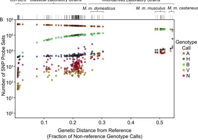
soft-ware [41]. We first hybridized 351 mouse DNA samples on the MDA. Those data are now public (http://cgd.jax.org/datasets/diversityarray/CELfiles.shtml), and include classical inbred strains, wild-derived strains, consomic strains, recombinant inbred strains, samples from early generations of the CC, F1 hybrids and wild mice – among the largest mouse genotype datasets available. Among the 143 inbred strains in that sample (116 classical and 27 wild-derived), we observed a significant increase in both heterozygous calls and no-calls as a function of genetic distance from the reference genome (Figure 2.4). All of those strains were expected to be fully homozygous based on previous studies (for at least 99% of their genomes), therefore we assumed that most of the heterozygous calls were errors (miscalls). We called genotypes for our sample set using three different algorithms: BRLMM-P 2D[63],Alchemy[64] and

MouseDivGeno. We found that genotype calls for the set of 351 samples were highly con-cordant in homozygous and heterozygous classes (97.4 - 97.8% agreement). The majority of discordant genotypes were due to homozygous calls using one of the methods that were called heterozygous using another method. Conflicts with opposite homozygous genotypes were very rare (less than 0.05% in all comparisons). The overall rate of AB genotypes was slightly lower forMouseDivGeno (10.26%) compared to Alchemy(11.45%) and BRLMM-P 2D

(11.62%). Of the VINO calls fromMouseDivGeno, 9.76% and 46.04% were called AB by

C57BL/6 Classical Laboratory Strains

M. m. domesticus

Wild-derived Laboratory Strains

M. m. musculus M. m. castaneus

106

A

B

105

104

103

102

101

100

Number of SN

P Probe Sets

0.1

Genetic Distance from Reference (Fraction of Non-reference Genotype Calls)

0.2 0.3 0.4 0.5

Genotype Call

A H B V N

Figure 2.4: Non-homozygous VINO call rates increase with divergence from the reference genome. A) Genetic distance from the mouse reference genome for 143 laboratory inbred strains. Each strain is shown as a vertical tick mark. Strains are grouped according to their origin are arranged left-to-right in increasing order of genetic distance from the reference. Genetic distance is computed as the fraction of non-reference (non-A allele) genotype calls. B) VINO calls for each strain. For each strain, the number of SNP probe sets assigned each of the five possible calls (A, B, H, V or N) are shown as five points of different colors that sum to 526,363 SNP probe sets.

strains.

that could not be aligned were inaccessible to SNP discovery and thus not comparable with array genotypes. The size of the inaccessible fraction of the genome increased with a strain’s divergence from the reference. I observed an enrichment of VINO calls in inaccessible regions of the Sanger data (2,221 VINO calls compared to an expectation of 54) [56], in probes with a deleted target base (24 vs. 2 expected) and unaligned or non-uniquely aligned probes (4,361 vs. 82 expected).

I examined the correlation between hybridization intensity and OTV position relative to the target SNP for the probes that had OTVs in at least one of the strains (Figure 2.5). I found that OTVs located within the first 3 bp of either the 5’ or 3’ end of a target sequence (edge OTVs) had relatively minor effect on hybridization intensity. In contrast, OTVs within the central region of the probe (central OTVs) had pronounced effect on hybridization intensity, with mean intensity differing by more than one standard deviation from that of probes having no OTVs. I also found that OTVs that disrupted a restriction fragment site and increased the size of the minimum fragment length to greater than 1500 bp significantly reduced hybridization intensities. I predicted from these results thatMouseDivGenowas undercalling VINOs by at least 1/3, since VINOs could not be recognized when the OTV was located in 6 of the 24 off-target positions. I determined the false-negative and false-positive rates for VINO calling by comparing predicted VINOs with the Sanger genotypes. Using the Sanger data as the “truth” was problematic due to miscalled or uncalled SNPs in that data set as well as known problems with the mouse genome assembly [66], but it was the best available metric. The measured false-negative rate for sequences with central OTVs was 55%. In most cases, false negatives were due to samples failing to meet the stringent requirements for VINO calling that were used to minimize the false-positive rate. The false-positive rate was 19.8%. I examined the performance ofAlchemyand BRLMM-Pand found a more than 30-fold increase in no-call rates for unexplained VINOs.

Log2(Mean Intensity)

A

B

Percent of Calls

0 10 20 30 40 50 60

C

E

D

OTV Position

Probe Sets

(Log10)

None0 1 2 3 4 5 6 7 8 9 10 11 12

Restriction Fragment Length

0 1 2 3 4 5 6

F

1000 2000 3000 4000

call

V N

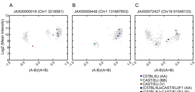
OTVs only alter one allele. Therefore, heterozygous genotypes with a nearby heterozygous OTV appeared as homozygous for the allele lacking the OTV. We called those “cryptic VI-NOs” (Figure 2.6). F1 hybrid mice were used to determine the extent of miscalls due to cryptic VINOs since their phase (i.e., parental origin) of haplotypes is known. We used a (C57BL/6JxCAST/EiJ)F1 with the expectation that all OTVs would be present only in the CAST/EiJ sequence. We found that 62% of SNPs with OTVs in heterozygosity were called as homozygous, leading to a low concordance rate (83.35%) between the genotypes predicted from the parental strains and the actual genotype calls for the F1 hybrid. Cryptic VINOs rep-resent a substantial source of genotyping error, particularly since they may only be recognized if the parental genotypes are known (and heterozygous parent genotypes will also be affected by cryptic VINOs).

6

C57BL/6J (AA) CAST/EiJ (BB) CAST/EiJ (V)

(C57BL/6JxCAST/EiJ)F1 (AA) (C57BL/6JxCAST/EiJ)F1 (N)

Log2 (Mean Intensity)

JAX00000018 (Chr1 3218581) JAX00009448 (Chr1 131687853) JAX00072427 (Chr16 91048133)

-1.0 -0.5 0.0 0.5 1.0 -1.0 -0.5 0.0 0.5 1.0 -1.0 -0.5 0.0 0.5 1.0

7 8 9 10 11 12 13

(A-B)/(A+B) (A-B)/(A+B)

(A-B)/(A+B)

A B C

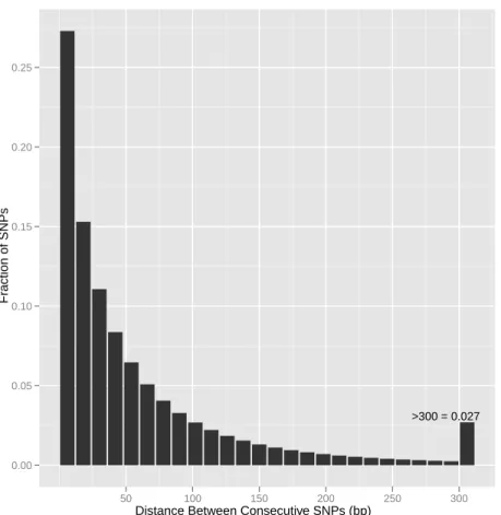
Distances between consecutive SNPs are expected to follow a geometric distribution (Fig-ure 2.7), with a significant proportion in the 0-12 bp range in species with high levels of vari-ation and large populvari-ations size such as the house mouse. In a significant fraction of probes with OTVs, we were able to detect the reduction in hybridization intensity and discriminate the samples harboring previously undetected variation from those that do not. VINOs are biased in favor of more divergent samples in reverse proportion to the degree to which the ge-netic variants in a given sample were known and represented on the array at the time of design. Thus VINOs could be used to counteract SNP selection bias (discussed further below).

Distance Between Consecutive SNPs (bp)

Fr

action of SNPs

0.00 0.05 0.10 0.15 0.20 0.25

>300 = 0.027

50 100 150 200 250 300

Figure 2.7: The distance between consecutive SNPs follows a geometric distribution. His-togram of distance between consecutive SNPs in 14 Sanger strains using a bin size of 12 bp. Distances greater than 300 bp are combined in the right-most bin.

testedMouseDivGenoon a randomly chosen subset of human HapMap data [67]. In 70% of cases,MouseDivGenoeither correctly called a VINO or the correct homozygous allele of the target variant. The 30% miscalls were all due to cryptic VINOs. We identified a 2:1 bias of VINOs in human YRI (Yoruban African) samples compared the other three HapMap popula-tions. That was consistent with the greater number of genetic variants in African populations that were unknown at the time of the design of the human SNP array.

2.6 Diagnostic SNPs

An important factor in the study of natural populations is the long-distance relatedness (shared ancestry) of individuals. At each SNP, two individuals may share the same allele or have different alleles. Shared alleles may be due to shared ancestry (identity by descent, IBD), or they may have occurred by recurring mutation (homoplasy). Alleles that are exclusive to a single taxa, or that only appear at a low level in other taxa due to homoplasy, are useful for determining the ancestral origin of previously uncharacterized individuals. We call such markers diagnostic alleles, although in studies of human ancestry they are sometimes referred to as ancestry-informative markers.

domesticus, M. m. musculusand M. m. castaneus, respectively. Those differences reflected the two opposing biases discussed above. On one hand, the selection criteria for inclusion of SNPs in the MDA led to the over-representation of SNPs withM. m. domesticus diagnostic alleles and under-representation ofM. m. castaneusSNPs [60]. On the other hand, the deeper knowledge of the genetic variation present in theM. m. domesticussubspecies allowed screen-ing of candidate SNP probes with internal polymorphisms that could create VINOs, whereas the limited knowledge of the genetic variation present in theM. m. castaneussubspecies in particular resulted in an excess ofM. m. castaneusdiagnostic VINOs. We constructed a phy-logenetic tree of the 36 wild-caught samples and confirmed the taxonomic classification of all samples (Figure 2.1).

The method described above allowed for misclassification caused by genotyping error, homoplasy or gene flow in the wild by down-weighting (but still considering diagnostic) al-leles that were detected at low frequency (< 5%) in the other subspecies. We are currently using a more robust method of identifying diagnostic alleles based on a Bonferroni-corrected Chi-squared test (2 df) for markers with significantly different frequencies in one subspecies compared to the other two. Diagnostic SNPs appear to be quite robust to sampling differ-ences. I applied the method for discovering diagnostic alleles to a larger sample and found 92% concordance with the set discovered in only 36 wild-caught mice.

2.7 VINOs and diagnostic SNPs mitigate ascertainment bias

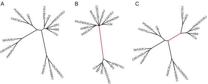
Ascertainment bias can result in distorted allele frequencies and inaccurate phylogenies. VINOs contain important phylogenetic information that can correct for the common problem of underestimating branch lengths for highly divergent samples due to missing information (which is typically ignored by phylogeny reconstruction methods). This is dramatically illus-trated by phylogenetic analysis of several different species of the Musgenus (Figure 2.8). I constructed maximum-likelihood phylogenetic trees using strains derived fromM. musculus,

methods). When only the standard genotypes were used, the discrimination between non-M. musculusspecies was poor (Figure 2.8 A). Furthermore, the length of the M. m. domesticus

branch was grossly overestimated while non-M. m. domesticusbranches were underestimated due to a high rate of missing information in those samples. The opposite result was observed when only VINOs were used to construct the tree by converting all genotypes to binary for the presence or absence of a VINO (Figure 2.8 B). When genotypes and VINOs were combined, discrimination between taxa increased and a representation more similar to morphology-based phylogenies emerged (Figure 2.8 C).

CIM POHN/Deh CAST/EiJ SKIVE/EiJ CZECHII/E PWK/PhJ PERC/EiJ WSB/EiJ ZALENDE/EiJ YCAXBS ZRU PANCEVO/EiJ SEG Ji E/ T E R P S SPRET/EiJ CIM POHN/Deh CAST/EiJ SKIVE/EiJ CZECHII/EiJ PWK/PhJ PERC/EiJ WSB/EiJ ZALENDE/EiJ YCA

XBS ZRUPANCEVO/EiJ SEG CIM POHN/Deh CAST/EiJ SKIVE/EiJ CZECHII/EiJ PWK/PhJ PERC/EiJ WSB/EiJ ZALENDE/EiJ YCAXBS ZRU PANCEVO/EiJ SEG Ji E/ T E R_P S

A B C

Figure 2.8: VINOs improve the topology of phylogenetic trees. Phylogenetic trees created using A) SNP genotypes only, B) VINOs only and C) both SNP genotypes and VINOs. The branch highlighted in red separatesM. musculusand non-M. musculusstrains and is the most significantly improved by the addition of VINOs.

2.8 Subspecific origin of laboratory mice

It has long been known that laboratory mice do not belong to a single taxa but rather represent a mosaic between multiple M. musculussubspecies [68, 50, 69]. Some have even suggested that the laboratory mouse be given it own taxonomic designation, Mus gemischus

domes-ticus and M. m. molossinus [46]. That view had a pervasive influence in the planning and interpretation of SNP discovery efforts.

We and others have recently presented results on the subspecific origin of laboratory mice using the newly available genotyping [55, 71, 40] and sequencing [56] platforms. The sets of strains used in those studies were different but highly overlapping. In each study, the authors chose one or more samples to serve as a reference for eachM. musculus subspecies. They then examined the local phylogenetic relationships among strains (called strain distribution patterns, SDPs) in small regions spanning the genome. Within each region, they attempted to assign a subspecific origin to each group of related strains based on the reference sam-ple(s) that clustered with the group. Remarkably, the local concordance between SDPs was high across all studies despite the use of distinct genotype data sets that differed in density by several orders of magnitude. However, in spite of the local agreement between phylogenetic relationships, the studies drew opposite conclusions about the ancestral origin of the labora-tory mouse genome. Frazer et al. (2007) concluded that the ratio of M. m. domesticus to non-domesticus (or unknown) ancestry in the classical strains was about 2:1, a finding that supported the traditional mosaic model. Their conclusions were based on the assumption that the four wild-derived strains were “pure” representatives of their respective subspecies. In contrast, Yanget al. (2007) determined that classical strains are primarily ofM. m. domesti-cusorigin (92%), with only a minor contribution fromM. m. musculusandM. m. castaneus

(6–7 and 1–2%, respectively). Their method was based on the use of diagnostic markers, and required excluding regions of the genome in which diagnostic markers were infrequent.

M. m. domesticus(mean of 94.3%±2.0% per genome), with variable contribution from M. m. musculus(5.4%±1.9%) and a small contribution fromM. m. castaneus(0.3%±0.1%). The contribution from subspecies other thanM. m. domesticus was not distributed randomly across the genome or among strains, but rather lay mostly in overlapping regions of strains with some shared history. Notably, theM. m. castaneus and M. m. musculus contributions were not independent from each other, with the former frequently nested within or contiguous with the latter. This association suggested aM. m. molossinusorigin of theM. m. musculus

contribution to the classical inbred strains. We tested this hypothesis by comparing theM. m. musculusregions found in classical inbred strains to wild-caughtM. m. musculusmice from Europe or Asia. Over 90% of theM. m. musculushaplotypes found in classical inbred strains clustered with Asian wild-caught mice.

Introgression is the movement of variants from one population into the gene pool of an-other population by the repeated backcrossing of a hybrid to one of its parent populations. Because M. musculus subspecies are not generally sympatric, introgression typically exists on a small scale and is difficult to observe, even with high-density genotype data. However, exceptions occur in places with a high rate of mixing between individuals of divergent ge-netic backgrounds [72]. Those regions are known as hybrid zones, and they may be natural or man-made. The derivation of new wild-derived strains has in large part been driven by a few fields of study, such as hybrid zone biology. This, along with the findings of [71] suggest that introgression may be widespread in wild-derived strains.

was a defining characteristic of derived laboratory strains as a group. Our set of wild-derived strains included ten strains wild-derived from natural intersubspecific hybrids, all of which had, unexpectedly, contributions from all three subspecies. The remarkable discordance in subspecific origin in several strains based on phylogeny (Figure 2.10) provides further evi-dence for intersubspecific introgression. Interestingly, we identified several shared patterns of subspecific origin between classical inbred strains and some wild-derived strains, which suggested that some of the intersubspecific introgressions in the latter group involved cross breeding with classical strains.

Diagnostic markers are also an important tool for identifying the ancestry of previously unstudied “new-world” populations (i.e., populations outside the historical ranges of the three subspecies). We obtained wild-caught mice from Southeast Farallon Island (USA) and Flo-reana Island (Galapagos archipelago, Ecuador). I used diagnostic markers to determine that both of these populations were primarilyM. m. domesticus. I analyzed the diagnostic markers using ChromoPainter [73] and identifed population structure and shared ancestry in M. m. domesticus mice. There were generally two genetically divergent populations: northern Europe and the Mediterranean basin. That reflected the general consensus that the mouse col-onized Europe from south to north, likely with partial isolation of the two populations due to geographic boundaries. The Farallon mice appear to be a mosaic of the northern and south-ern populations. I constructed separate phylogenies of the mitochondrial and Chr Ys of the samples and found that the Farallon mice clustered with mice from the northern UK in the former, and the Mediterranean basin in the later. Together, this evidence suggests multiple colonizations of the Farallon Islands by house mice of different origins.

2.9 Haplotype and sequence diversity

Figure 2.9: The phylogeny of derived strains. Neighbor-joining phylogeny of 62 wild-derived strains based on SNP and VINO genotypes. Node colors represent bootstrap values. The outer ring of colors shows the fraction of the genome of each strain that is derived from

within subsets of strains. A natural criterion to define haplotype blocks in classical strains is to identify regions of shared ancestry among multiple strains which have not recombined (compatible intervals) [74, 40] using the 4-gamete rule [75]. We used the 4-gamete rule to identify 43,285 haplotype blocks with a median size of 71 kb in 100 classical strains. The majority of blocks contained between four and six haplotypes, and there were fewer than ten haplotypes across 97% of the genome. Those findings confirmed the small size of the classi-cal strain founder population. The larger numbers of haplotypes in the remaining 3% of the genome were due to a combination of new mutations in the past century and contributions from outside of the founder population. Blocks with large numbers of different haplotypes should be further investigated to understand their origins.

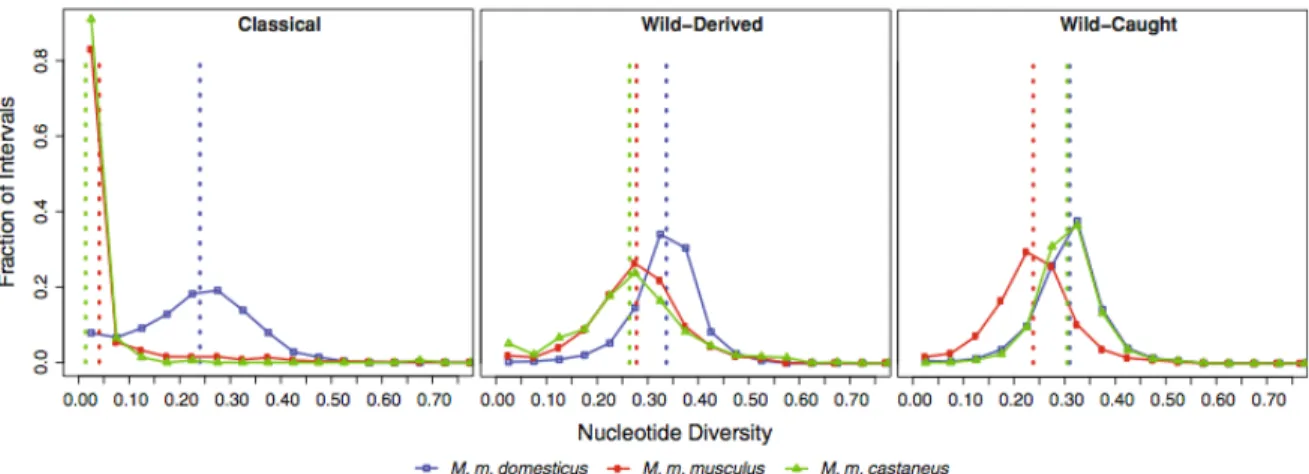
The relative lack of genetic variation in classical strains limits their utility in at least two respects. First, it constrains the phenotypic variation that exists in classical strains. Second, use of classical strains is inappropriate to study evolutionary processes since they may be invariant for many of the genes involved in speciation [76]. The extent of additional variation present in natural populations of M. musculus is hinted at by limited studies in wild mice [77] and by the recent whole-genome sequencing of three wild-derived strains [56], but it is not known for certain. To examine sequence variation at the genome scale, I computed the nucleotide diversity in classical, wild-derived, and wild-caught mice. I used the method of [78] to compute the average pairwise genetic distance between individuals within a population

π. Overall, I found greater diversity in wild-derived and wild mice than in classical strains (π = 0.298, 0.282, and 0.203, respectively). The contrast is even more striking, however, when comparing diversity between regions with different subspecific origin (Figure 2.10). In classical strains, intervals derived from M. m. domesticus founders had 6 and 17 times greater diversity than intervals derived from the minority Asian fancy mouse founders (M. m. musculus andM. m. castaneus, respectively, Figure 2.10 A), whereas in wild-derived lines and wild mice (Figures 2.10 B,C), variation is similar among regions of different ancestry.

hap-Figure 2.10: Nucleotide diversity is greater in wild mice than classical strains. We divided the genome into 16,331 intervals with no historical evidence of recombination in classical strains and measured nucleotide diversity (π) at diagnostic SNPs in each interval for classical strains, wild-derived strains, and wild-caught mice. The x axis shows π for each subspecies in bins of 0.01. The y axis shows the fraction of intervals with the given subspecific origin that is in each bin. Vertical dotted lines show mean values of π for each subspecies. Color indicates subspecific origin. Blue:M. m. domesticus; red: M. m. musculus; green:M. m. castaneus.

lotype diversity are not accounted for [79, 80]. Haplotype structure also has important impli-cations for the ability to conduct genetic mapping because it can significantly affect the level and rate of decay of linkage disequilibrium (LD) [39]. Gametic disequilibrium (GD), which is also known as long-range LD, is problematic because it can introduce false genotype– phenotype associations [81, 82]. An analysis of LD decay in a panel of 88 classical strains revealed widespread GD [39], suggesting caution when interpreting the results of mapping experiments in those strains. The effect of population structure can be reduced by using a genetic reference population (such as the CC).

2.10 The MegaMUGA genotyping array

preparation protocols compared to the MDA. The array contained 7,851 SNP markers that were distributed throughout the mouse genome. The markers were chosen to be maximally informative and maximally independent for the eight founder strains of the CC. Informative-ness was determined by minor-allele frequency, and independence was determined by local pairwise linkage disequilibrium. The design criteria resulted in sets of three contiguous SNPs that together could uniquely identify each of the eight founders. The design was also optimal for the detection of heterozygous regions in the CC.

2.11 Studies using the MegaMUGA array

I conducted several experiments that demonstrate the versatility of the MegaMUGA ar-ray. I first assessed the genotyping error rate of MegaMUGA and found it to be remarkably low (0.04%) when comparing biological replicates of 11 inbred lines. I also compared those samples to the Sanger genotypes and found an inconsistency rate of 2.1%. I hypothesized that most inconsistencies were systematic, either due to incorrect Sanger genotypes or poorly performing MegaMUGA probes. When I eliminated the 4,052 poorly-performing markers (5.2% of markers), the rate of inconsistency fell to 0.005%. I developed a set of QC met-rics for determining the quality of array data (described in Appendix A). I implemented these methods in an R package,megamugaQC, that will be released along with the publication on the MegaMUGA array.

on MDA data. All wild-caught animals were classified as completely pure representatives of their predicted subspecies. For inbred strains, most small introgressions (<0.5 Mb) were not identified. Large introgressions were identified as a deviation from the predicted subspecies, but the subspecific origin was often assigned incorrectly (usually as a mixture of two sub-species). Those results were expected due to the relatively low density ofM. m. musculusand

M. m. castaneusdiagnostic alleles.

While the genotypes for Chr Y and mitochondrial markers were robust, the relatively small number of markers made phylogenetic analysis problematic. I examined the intensity data and found a large number of additional sample clusters (i.e., VINOs) that were important to producing correct phylogenies. Since the VINO identification method has not yet been extended to MegaMUGA, I performed supervised clustering of 44 mitochondrial and 38 Chr Y probes that were both unique and had multiple distinct clusters. I randomly assigned non-allelic genotypes to the clusters beyond the two expected alleles. I created parsimony trees using the DNAPARS program in the Phylippackage [84]. The Chr Y phylogeny yielded a single best tree, while the mitochondrial phylogeny yielded multiple best trees. I analyzed each SNP independently using a test for leaf node proximity [85] and found that 26 of the mitochondrial markers (59%) showed evidence of homoplasy; only 9 Chr Y markers were homoplasic (24%). This high level of homoplasy in the mitochondrial tree was expected because the majority of the mitochondrial SNPs on MegaMUGA are located in the D-loop region, which has an extremely high mutation rate [86].

Significant increases or decreases in intensity across consecutive probes are indicative of copy number variation (CNV). MUGA and MegaMUGA have been important for us and oth-ers as a tool to study multiple types of CNV. In creating the Chr Y phylogeny, I uncovered intra-specific variation in the pseudo-autosomal region (PAR) of the Chr Y. The PAR is a

longer than in other mouse strains. However, intensity data showed that, inM. m. castaneus

mice from Taiwan, the region of homology extended less than 100 kb beyond the ancestral boundary. Furthermore, recombination data from the CC showed that 90% of recombinations involving CAST/EiJ PARs were within the ancestral PAR, 10% were within the 100kb proxi-mal to the ancestral PAR, and no recombinations occurred in the other 330kb of the CAST/EiJ region of homology. This finding suggests that the CAST/EiJ PAR evolved through two sepa-rate events: first a duplication of∼100kbof Chr X sequence in the ancestralM. m. castaneus

lineage, followed by a second duplication event exclusive to some subset of southeast Asian mice that happened after they diverged with the Taiwanese population. This lends further support to the finding thatM. m. castaneusis polytypic [87].

In another study, I surveyed 100 mouse cell lines using the GAP algorithm [88] and found that a large fraction of lines (15%) had evidence of whole-chromosome loss or gain for at least one chromosome.

I also developed a method to distinguish male and female samples based on their X- and Y-chromosome intensity profiles, and simultaneously detect sub-chromosomal CNV. Briefly, I used a supervised method based on predicted sex to identify sex-specific intensity distributions for each marker. I then determined the probability that a sample belongs to each distribution within a moving SNP window, and I identified intervals of consistent copy number predic-tion. I predicted the baseline chromosome copy number from the relative local copy-number rates. I used this method to predict the sex of approximately 5,000 MegaMUGA arrays in our database. I identified 27 samples with obviously incorrect reported sexes. I also identified 33 females having a single Chr X (XO, Figure 2.11). Interestingly, the frequency of XOs is much higher in the DO population than in other laboratory strains or wild mice. This finding is the subject of ongoing investigation.