PubMedCentral-PMC5310887.pdf

(1)

Nearest shrunken centroids via alternative

genewise shrinkages

Byeong Yeob Choi1,2_{, Eric Bair}2,3_{, Jae Won Lee}4

*

1 Department of Epidemiology and Biostatistics, University of Texas Health Science Center, San Antonio, TX, United States of America, 2 Department of Biostatistics, University of North Carolina, Chapel Hill, NC, United States of America, 3 Department of Endodontics, University of North Carolina, Chapel Hill, NC, United States of America, 4 Department of Statistics, Korea University, Anam-Dong, Seoul, South Korea

*[email protected]

Abstract

Nearest shrunken centroids (NSC) is a popular classification method for microarray data. NSC calculates centroids for each class and “shrinks” the centroids toward 0 using soft thresholding. Future observations are then assigned to the class with the minimum distance between the observation and the (shrunken) centroid. Under certain conditions the soft shrinkage used by NSC is equivalent to a LASSO penalty. However, this penalty can pro-duce biased estimates when the true coefficients are large. In addition, NSC ignores the fact that multiple measures of the same gene are likely to be related to one another. We consider several alternative genewise shrinkage methods to address the aforementioned shortcom-ings of NSC. Three alternative penalties were considered: the smoothly clipped absolute deviation (SCAD), the adaptive LASSO (ADA), and the minimax concave penalty (MCP). We also showed that NSC can be performed in a genewise manner. Classification methods were derived for each alternative shrinkage method or alternative genewise penalty, and the performance of each new classification method was compared with that of conventional NSC on several simulated and real microarray data sets. Moreover, we applied the geomet-ric mean approach for the alternative penalty functions. In general the alternative (genewise) penalties required fewer genes than NSC. The geometric mean of the class-specific predic-tion accuracies was improved, as well as the overall predictive accuracy in some cases. These results indicate that these alternative penalties should be considered when using NSC.

Introduction

Nearest shrunken centroids (NSC) is one of the most frequently used classification methods for high-dimensional data such as microarray data [1,2]. NSC shrinks the average expression (i.e., centroid) of each gene within each class toward the overall centroid via soft thresholding. Genes whose expression levels do not significantly differ between the classes will have their centroids reduced to the overall centroids, effectively removing them from the classification procedure. The amount of shrinkage is determined by cross validation. Then class prediction a1111111111

a1111111111 a1111111111 a1111111111 a1111111111

OPEN ACCESS

Citation: Choi BY, Bair E, Lee JW (2017) Nearest

shrunken centroids via alternative genewise shrinkages. PLoS ONE 12(2): e0171068. doi:10.1371/journal.pone.0171068

Editor: Lars Kaderali, Universitatsmedizin

Greifswald, GERMANY

Received: August 4, 2016

Accepted: January 16, 2017

Published: February 15, 2017

Copyright:©2017 Choi et al. This is an open access article distributed under the terms of the Creative Commons Attribution License, which permits unrestricted use, distribution, and reproduction in any medium, provided the original author and source are credited.

Data Availability Statement: All relevant data are

within the paper and its Supporting Information files.

Funding: This work was supported by the National

Research Foundation of Korea (NRF) grant funded by the Korea government (MSIP) (No.

2016943438). Eric Bair was partially supported by NIH/NIDCR grant R03DE02359, NIH/NCATS grant UL1RR02574, and NIH/NIEHS grant P03ES01012.

Competing interests: The authors have declared

(2)

is performed using the shrunken centroids, which allows one to identify important genes and predict the class of unlabeled observations.

Wang and Zhu [3] showed that NSC is the solution to the regression problem that estimates the class centroids subject to anL1penalty (i.e., LASSO) of Tibshirani [4]. They observed that

the LASSO penalty applies the same penalties to all centroids, but the centroids for the same gene should be treated as one group. To overcome this problem, they proposed two NSC methods using different penalties: adaptiveL1-norm penalized NSC (ALP-NSC) and adaptive

hierarchically penalized NSC (AHP-NSC). They showed that the two NSC methods have bet-ter performance than the original NSC in bet-terms of misclassification error rate and the number of variables with nonzero centroids. However, ALP-NSC requires an exhaustive search to find an index set satisfying certain condition. If no such indices exist, quadratic programming must be employed to estimate the parameters. AHP-NSC requires an iterative procedure to estimate the parameters, and this increases the computational burden as the number of genes increases.

While Wang and Zhu [3] sought to improve NSC by considering the correlation between the centroids for the same gene, Guo et al. [5] improved NSC by regularizing the covariance matrix of genes in addition to shrinking the class centroids. In fact, Guo et al. [5] modified the classical linear discriminant score, not the diagonal linear discriminant score, and thus the method of Guo et al. [5] is a generalized version of NSC. Pang et al. [6] proposed an improved diagonal linear discriminant analysis (LDA) through shrinkage and regularization of the vari-ances, but their method dose not perform variable selection. Several authors proposed new types of sparse LDA and provided the related optimality conditions and asymptotic properties. Shao et al. [7] applied the thresholding methodology, which was developed for function esti-mation, to the estimation of the means and variances, and Mai et al. [8] used the least squares formulation of LDA.

Another way to improve NSC is to modify the way to select an optimal threshold as in Bla-gus and Lusa [9]. They improved NSC in class-imbalanced data by selecting the optimal threshold as the value that maximizes the geometric mean of the class-specific prediction racies. Their numerical studies showed that the modified NSC improved the prediction accu-racy of the minority class and area under the curve (AUC), and even the average prediction accuracy of entire classes for some real data.

In this article, we proposed the methods that improve NSC through alternative shrinkage of the class centroids. Like Wang and Zhu [3], we used an additional parameter, which controls the amount of penalization given to the parameters for our methods. These alternative shrink-ages were derived from three existing alternative penalized regression methods, namely the smoothly clipped absolute deviation (SCAD) [10], the adaptive LASSO (ADA) [11], and the minimax concave penalty (MCP) [12], which are known to outperform LASSO regression in some situations. They enjoy the oracle property, which means that the efficiency of these esti-mators is not reduced when the subset of variables with nonzero coefficients is unknown. As noted earlier, under an orthonormal design (such as the case of NSC), the LASSO solution can be obtained via soft thresholding. Similarly, these three regression methods also have simple solutions in the NSC setting, so the computation is easy and fast. While the LASSO solution yields biased estimates for large coefficients, these methods produce unbiased estimates. Sev-eral researchers have considered the use of the alternative shrinkage methods in place of soft shrinkage [2,13,14]. In this article, we will evaluate the performances of these alternative shrinkage methods by comparing them with conventional soft shrinkage systematically through simulation and real data studies.

(3)

the fact that the centroids from the same gene should be treated as a group, but they are less computationally intensive than those of Wang and Zhu [3] because an iterative procedure is not involved. The approach of Blagus and Lusa [9] was also applied for our alternative (gene-wise) penalties to further improve NSC, especially for class-imbalanced data.

In the Methods section, we described the penalized least squares framework for general shrinkage methods using the model of Wang and Zhu [3], which includes the special case of NSC. We examined the performance of NSC with alternative penalty functions (ALT-NSC), which include the SCAD, the adaptive LASSO and the MCP. We also described how ALT-NSC can be used for genewise inference (GEN-NSC). In the Simulation section, we conducted sim-ulation studies and showed that ALT-NSC and GEN-NSC have substantially better perfor-mance than NSC in terms of predictive accuracy and feature selection in data sets with multiple classes. In the Real Data Study section, we applied the proposed variants of NSC to several real microarray data sets. A discussion and concluding remarks are provided in the last two sections.

Methods

Penalized least squares for the nearest shrunken centroids

Adapting the framework of Wang and Zhu [3], letxijbe the gene expression for thejth gene of theith sample (j= 1,. . .,p;i= 1,. . .,n). There areKclasses and each sampleibelongs to one of

Kclasses, that isi2Ck, whereCkis the set of sample indexes belonging to classk2{1,. . .,K}, andnkis the number of samples for classk. The average expressions for thejth gene in thekth class and over the entire data set arexkj ¼

P

i2Ckxij=nkandxj¼

P_n

i¼1xij=nrespectively.

Let

m0 kj¼

xkj xj

mksj

;

wheresjis the pooled within-class standard deviation for thejth gene:

s2 j ¼

1

n K

XK

k¼1 X

i2Ck

ðxij xkjÞ 2

;

andmk¼

ffiffiffiffiffiffiffiffiffiffiffiffiffiffiffiffiffiffiffiffiffiffiffi

1=nk 1=n p

. Alternatively,sj+s0can be used instead ofsjto prevent the genes with low expression levels from having largem0

kjvalues by chance due to very smallsjvalues,

wheres0is a small constant. The statisticm0kjis equivalent todkj, in Tibshiraniet al. [1,2], which is a t-statistic for thejth gene comparing classkto the average of the other classes.

Letyij¼ ðxij xjÞ=ðmksjÞand consider the following linear model:

yij¼ XK

k¼1

zikmkjþεij; ð1Þ

wherezik= 1 if sampleibelongs to the classk, and 0 otherwise,μkjis a parameter to be esti-mated andεijis an independent error term that has variance1=m2kif sampleibelongs to class

k. For a fixed gene indexj,μkjis a deviation from the overall mean, so we have the constraint thatPK_k¼1mkj¼0. The class index to which sampleibelongs is denoted byk(i)2{1,. . .,K}. By

multiplying1= ffiffiffiffiffiffiffiffinkðiÞ

p

to both sides inEq (1), we have

y

ij¼ XK

k¼1

zik ffiffiffiffiffiffiffiffi nkðiÞ

p mkjþε

(4)

wherey

ij¼yij= ffiffiffiffiffiffiffiffi nkðiÞ

p

andε

ij¼εij= ffiffiffiffiffiffiffiffi nkðiÞ

p

. In vector notation,Eq (2)can be written as

y_¼_W_μ_þ_ε_;

where

y _¼ y11 ffiffiffiffiffiffiffiffi n_kð1Þ

p ; yffiffiffiffiffiffiffiffi_n12 kð1Þ

p ; :::; yffiffiffiffiffiffiffiffi_n1p kð1Þ

p ; yffiffiffiffiffiffiffiffi_n21 kð2Þ

p ; :::; yffiffiffiffiffiffiffiffi_nnp kðnÞ

p !T

;

ε _¼ ε11

ffiffiffiffiffiffiffiffi nkð1Þ

p ; εffiffiffiffiffiffiffiffi12 nkð1Þ

p ; :::; εffiffiffiffiffiffiffiffi1p nkð1Þ

p ; εffiffiffiffiffiffiffiffi21 nkð2Þ

p ; :::; εffiffiffiffiffiffiffiffinp nkðnÞ

p !T

;

μ ¼ ðm11;m12; :::;m1p;m21; :::;mKpÞ T

;

μ0

¼ ðm0 11;m

0 12; :::;m

0 1p;m

0 21; :::;m

0 KpÞ

T

;

whereATdenotes the transpose of a vector or matrixA. The design matrix W = (W1,. . ., WKp) is annp×Kpmatrix, where Wlis anp× 1 vector that corresponds to thelth element of the vec-torμforl= 1 ,. . .,Kp. If an indexlbelongs to a class indexkand a gene indexj, thennk(i)

ele-ments of Wlare1= ffiffiffiffiffiffiffiffinkðiÞ

p

and the rest of the elements are zeros because there are exactlynk(i)

samples belonging to classk(i). This implies thatWT

lWl¼1ðl¼1; :::;KpÞ. In addition, we

can see that each row of W has only one non-zero value and the rest of the elements are zero. This is because eachyijtakes only oneμkj, and this impliesWlTWh¼0for (l6¼h). Thus, W is

orthonormal. Note thatμ0= WTy_{is the least squares estimator for}_μ_{, and let}_^_y_¼_W_μ0_{. Since}

W is orthonormal, a form of the penalized least squares is given by [10]:

1 2ky

_Wμ

k2

þlX

p

j¼1 XK

k¼1

pðjm_kjjÞ

¼1 2ky

^

yk2

þ1 2

Xp

j¼1

XK

k¼1ðm 0 kj mkjÞ

2

þXp

j¼1

XK

k¼1plðjmkjjÞ;

ð3Þ

wherepλ() =λp() is a penalty function andkAk2 ¼ P_n

i¼a

2

i whenA= (a1,. . .,an)

T_{. The}

problem of minimizingEq (3)with respect toμkjis equivalent to minimizing it component-wise. By ignoring1

2ky

_^_y_k2_{, which is irrelevant to the parameters, this allows us to}

con-sider the following penalized least squares problem:

1 2ðm

0 kj mkjÞ

2

þplðjmkjjÞ: ð4Þ

Eq (4)shows that the minimization problemEq (3)has been converted to a univariate min-imization problem. Since, the univariate solutions for regression coefficients are presented in the papers describing these penalized regression methods, we can use these solutions to obtain ^

m_kj. NSC uses the LASSO penalty functionpλ(|μkj|) =λ|μkj| [4], and the resulting estimator for

μkjis given by

^

m_kj¼sgnðm0 kjÞðjm

0 kjj lÞþ;

where “sgn” is a sign function andz+is the positive part ofz. The LASSO solution is equivalent

(5)

To predict the class of a new samplex_{¼ ð}_x

1; :::;x

pÞ T

, we define the discriminant score for

classkas

d_kðx_{Þ ¼}X

p

j¼1 ðx

j ^xkjÞ 2

s2 j

2logp_k;

where^xkj¼xjþm^kjmksjis a shrunken mean andπk=nk/nis a prior probability estimate for classk. The shrunken mean and the discriminant score depend on the shrinkage method used, hence the choice of shrinkage method affects class prediction and gene selection. Finally, the classification rule is given by

Cðx_{Þ ¼}_k_; _where _k_¼ _{arg min}

k dkðx

Þ:

Alternative shrinkage methods (ALT-NSC)

Here, we described several shrinkage methods that are possible alternatives to soft shrinkage. The first order derivative of the SCAD penalty function [10] is defined as

p0

l;aðjmkjjÞ ¼l Iðjmkjj lÞ þ

ðal m_kjÞ_þ

ða 1Þl Iðjmkjj>lÞ

;

for somea>2. This penalty function gives smaller penalties on larger coefficients. The result-ing estimator forμkjis

^ m_kj¼

sgnðm0 kjÞðjm

0

kjj lÞþ; if jm

0 kjj 2l

ða 1Þm0

kj sgnðm 0 kjÞal

a 2 ; if 2l<jm 0 kjj al

m0

kj; if jm

0 kjj>al: 8 > > > > > < > > > > > :

Ifais close to 2, then SCAD behaves like a hard shrinkage estimate when estimatingμkj. The adaptive LASSO penalty function [11], which is the LASSO penalty function with a data-dependent weight, is given by

pl;aðjmkjjÞ ¼ljmkjj=jm 0 kjj

a

;

wherea>0. The resulting solution is

^

m_kj¼sgnðm0 kjÞðjm

0

kjj l=jm 0 kjj

a Þ_þ;

or

^ m_kj¼m0

kjð1 l=jm 0 kjj

aþ1 Þ_þ:

The adaptive LASSO solution is equivalent to soft shrinkage whena= 0 and is similar to the nonnegative garotte whena= 1 [17] (although the nonnegative garotte requires additional sign restrictions).

The MCP penalty function [12] is defined as

pl;aðjmkjjÞ ¼

ljm_kjj m2

kj=ð2aÞ; if jmkjj al;

0:5al2; if jm_kjj>al; 8

<

(6)

wherea>1. The resulting solution is given by

^ m_kj¼

sgnðm0 kjÞðjm

0 kjj lÞþ 1 1=a ; if jm

0 kjj al;

m0

kj; if jm

0 kjj>al: 8

> > <

> > :

The MCP solution is equivalent to firm shrinkage, which offers advantages over soft and hard shrinkage [18]. The MCP solution approaches hard shrinkage asa!1 and soft shrinkage asa! 1.

As mentioned previously, these shrinkage methods are known to have oracle properties under some mild conditions (for details, see [10], [11] and [12]). The LASSO solution is incon-sistent because it produces estimates biased toward zero. This bias in the LASSO can also cause its variable selection to be inconsistent [12]. The basic reason that the alternative shrink-ages can produce better estimates is because they have different rules for estimating the coeffi-cientsμkj, which depend on the size of |μkj|. When the sizes of the coefficients are large, these procedures leave them almost unpenalized (or completely unpenalized). Thus, they overcome the tendency of soft shrinkage to produce biased estimates.

While soft shrinkage has one tuning parameterλ, the alternative shrinkage methods have two tuning parameters, namelyaandλ. The tuning parameteracontrols the size of the penal-ties for large coefficients. The tuning parameters are determined by cross validation (CV). In our subsequent analysis, six values of the tuning parameterawere examined for each ALT-NSC and genewise shrinkage method: (0.5, 1, 1.5, 2, 2.5, 3) for the adaptive LASSO pen-alty, (2.01, 2.2, 2.5, 2.8, 3.2, 3.7) for the SCAD penalty and (1.01, 1.3, 1.7, 2, 2.5, 3) for the MCP penalty. For each method, thirty values ofλwere considered. For the case when there are ties among the CV prediction accuracies or g-means, we chose the parameters resulting in a smaller number of genes.

Genewise shrinkage methods (GEN-NSC)

Here we extend the shrinkage methods discussed in the previous subsection to genewise infer-ence. Letμj= (μ1j,. . .,μKj)Tdenote aK× 1 mean vector for thejth gene. Further letμ0j ¼

ðm0 1j; :::;m

0 KjÞ

T

denote the corresponding mean estimator vector. The objective function to be minimized for the genewise penalized least squares estimator is

1 2ky

Wμk2

þlX

p

j¼1

pðkμ_jkÞ: ð5Þ

Note that instead of penalizingμkj, we penalize the vectorμj. Using the fact that

Xp

j¼1 XK

k¼1 ðm0

kj mkjÞ 2

¼X

p

j¼1 kμ0

j μj k 2

and the orthonormality of W,Eq (5)can be written as

1 2ky

_y_^_k2_þ1 2

Xp

j¼1 kμ0

j μjk 2_þX

p

j¼1

(7)

The solution toEq (6)is genewise separable, and thus one may solve it by minimizing

1 2kμ

0 j μjk

2

þplðkμj kÞ: ð7Þ

Using the result of Antoniadiset al. [15], the solution toEq (7)is given by

^

μ_j¼rðkμ0 j kÞμ

0 j=kμ

0

j k; ð8Þ

whererðkμ0

j kÞis the solution to

min

r fðkμ 0 jk rÞ

2

þplðrÞg: ð9Þ

SinceEq (8)depends on the penalty functionpλ(), we can derive genewise shrinkage

meth-ods under diverse penalty functions. Note that the problem of solvingEq (9)is equivalent to that ofEq (4), and thus, the computational complexity of the genewise shrinkages is the same as that of the alternative shrinkages.

When the LASSO penalty is employed,

^

μ_j¼μ0

jð1 l=kμ 0 jkÞþ:

If the SCAD penalty is used,

^

μ_j ¼

μ0

jð1 l=kμ 0

jkÞþ; if kμ

0 j k2l;

ða 1Þ kμ0 j k al ða 2Þ kμ0

j k

μ0

j; if 2l<kμ 0 j kal;

μ0

j; if kμ

0 j k>al; 8 > > > > > > < > > > > > > :

wherea>2. For the adaptive LASSO penalty, the resulting solution is

^

μj ¼μ 0

jð1 l=kμ 0 jk

aþ1_Þ

þ:

For the MCP penalty,

^

μ_j¼

μ0

jð1 l=kμ 0 jkÞþ

1 1=a ; if kμ

0 j kal;

μ0

j; if kμ

0 j k>al; 8 > > < > > :

wherea>1.

The thresholding rules of the genewise shrinkage methods are determined bykμ0

j kinstead

of an individualm0

kj. By pulling information from the neighboring mean estimators belonging

to the same gene, the genewise shrinkage may allow the accuracy of the thresholding mean estimators to be improved. Furthermore,Eq (5)has a nice Bayesian interpretation [15]: the genewise penalized least squares method models the mean coefficients belonging to the same gene by using proper prior distributions.

Geometric mean methods (GM)

(8)

Throughout the remainder of this manuscript, we will refer to the genewise version of each method by adding “G” to the beginning of its abbreviated name. Moreover, when the tuning parameters are determined by the geometric mean, we will add “GM-” to the beginning of the name. For example, “GADA” refers to the genewise version of adaptive lasso, and “GM-GADA” referes to “GADA” whose tunnig parameters are determined by the geometric mean.

Simulations

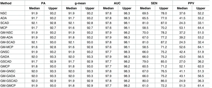
In this section, we conducted simulation studies to compare ALT-NSC, GEN-NSC, and the GM versions of ALT-NSC and GEN-NSC to conventional NSC. We examined the overall pre-diction accuracy (PA), geometric mean (g-mean), area under the curve (AUC, only for a two-class two-classification scenario), sensitivity (SEN) and positive predictive value (PPV). SEN is the number of detected important genes divided by total number of important genes. PPV is the number of detected important genes divided by total number of genes the method selects. As in Dudoit et al. [19], we presented the median and upper quartiles of the evaluation measures.

In a two class classification scenario, we generated two classes from multivariate normal distributions with sample sizes,n1=nπ1andn−n1: MVN(μ1,S) and MVN(μ2,S), each had a

dimension ofp= 2500.μ1was equal to 0 for all genes andμ2was 0.5 for 100 genes and 0 for

the rest of genes. The differentially expressed (DE) 100 genes were randomly selected. As in Guo et al. [5] and Pang et al. [6],Swas a block diagonal matrix with each diagonal blockSρ having an auto-regressive structure and alternating in sign. The block size was 50× 50 and there were 50 blocks, which gave a total of 2500 genes:

Sr¼

1 r r48 _r49

r 1 .. . r48

.. .

. . .

.. .

r48

.. . 1 r

r49 _r48 _r ₁ 0

B B B B B B B B B B B B B @

1

C C C C C C C C C C C C C A :

ρtook values of 0.5 and 0.9, indicating sparse and dense correlation blocks, andπ1took values

of 0.5 and 0.8, corresponding to class-balance and -imbalance.

The three class classification scenario is very similar to the previous one. We generated three classes from multivariate normal distributions with the fixed proportions (π1,π2,π3) =

(0.4, 0.2, 0.4): MVN(μ1,S), MVN(μ2,S) and MVN(μ3,S), each of which had the same

dimen-sion as the previous scenario. Ninety differentially expressed genes were randomly selected and those DE genes had mean vectors of (γ, 0,−γ). We used the sameSas in the first simula-tion. We letγtake the values of 0.5 and 0.1 to study how the effect size of DE genes is related to the performances of the classifiers.

(9)

Simulation results for the two-class scenario have been presented in Tables1,2,3and4. All of the proposed methods performed very similarly to NSC in terms of PA, g-mean and AUC except when the diagonal block matrix was dense and class was imbalanced; ALT-NSC improved the g-mean slightly, the GM versions of ALT-NSC and GEN-NSC also improved the

Table 1. Two groups with sparse block diagonal structure (ρ= 0.5) and class-balance (π1= 0.5).

Method PA g-mean AUC SEN PPV

Median Upper Median Upper Median Upper Median Upper Median Upper

NSC 91.9 93.2 91.9 93.2 97.8 98.3 69.5 78.0 37.6 52.2

ADA 91.7 93.2 91.7 93.2 97.8 98.3 65.5 77.0 41.5 55.2

SCAD 92.1 92.8 92.1 92.8 97.8 98.1 81.0 87.0 24.3 33.1

MCP 91.7 92.7 91.6 92.7 97.6 98.1 58.5 70.2 53.1 64.4

GM-NSC 91.9 93.2 91.9 93.2 97.9 98.2 70.0 78.2 37.2 51.0

GM-ADA 91.9 93.2 91.8 93.2 97.9 98.3 67.0 77.2 39.2 53.2

GM-SCAD 92.1 93.0 92.1 93.0 97.8 98.1 81.0 87.2 24.3 32.4

GM-MCP 91.6 92.8 91.6 92.8 97.6 98.1 58.5 71.2 52.6 64.1

GNSC 91.9 93.2 91.9 93.2 97.7 98.3 66.0 75.2 42.4 51.9

GADA 92.0 93.3 92.0 93.3 97.9 98.3 66.0 75.2 43.0 56.5

GSCAD 91.7 92.9 91.7 92.9 97.7 98.2 79.0 85.0 27.0 36.2

GMCP 91.8 93.0 91.8 93.0 97.7 98.2 60.5 71.2 52.1 62.0

GM-GNSC 92.0 93.3 92.0 93.3 97.8 98.3 67.0 76.5 41.1 51.3

GM-GADA 92.0 93.3 92.0 93.3 97.9 98.3 66.0 75.2 43.1 56.5

GM-GSCAD 92.0 92.9 91.9 92.9 97.8 98.2 80.0 86.0 24.9 36.3

GM-GMCP 91.9 93.0 91.8 92.9 97.7 98.2 61.0 72.2 51.3 61.4

“PA”, “g-mean” and “AUC” are overall accuracy, geometric mean and AUC of class prediction, calculated from the test data set. “SEN” and “PPV” are sensitivity and positive predictive value of gene selection obtained from the training data set. “Median” and “Upper” are median and upper quartiles of 100 repetitions. The scale of all the numbers is a percentage.

doi:10.1371/journal.pone.0171068.t001

Table 2. Two groups with dense block diagonal structure (ρ= 0.9) and class-balance (π1= 0.5).

NSC 85.8 88.1 85.7 88.1 93.4 95.4 46.0 57.0 68.4 81.4

ADA 86.1 88.7 86.1 88.7 93.4 95.5 44.0 57.0 71.9 81.4

SCAD 85.3 87.8 85.3 87.8 93.1 95.1 51.5 65.0 61.5 78.3

MCP 86.0 88.6 86.0 88.6 93.5 95.6 34.5 47.0 81.8 90.7

GM-NSC 85.9 88.4 85.9 88.4 93.6 95.4 48.5 58.5 64.6 79.0

GM-ADA 86.1 88.6 86.1 88.5 93.4 95.5 45.0 59.0 69.0 80.1

GM-SCAD 85.3 87.9 85.3 87.9 93.3 95.1 54.0 66.2 60.2 72.7

GM-MCP 86.3 88.6 86.3 88.6 93.7 95.6 36.0 48.0 81.4 91.2

GNSC 85.0 87.9 85.0 87.9 93.1 95.2 47.0 54.0 69.9 81.9

GADA 84.8 88.0 84.8 88.0 92.9 95.3 45.0 55.0 73.0 83.8

GSCAD 84.3 87.1 84.3 87.1 92.9 94.5 50.0 64.2 63.5 80.9

GMCP 84.2 88.2 84.2 88.2 92.4 95.5 34.5 47.2 81.2 94.9

GM-GNSC 85.0 87.8 85.0 87.8 93.1 95.2 48.0 56.5 66.7 81.9

GM-GADA 84.7 88.3 84.7 88.3 92.8 95.3 44.5 55.0 72.3 83.8

GM-GSCAD 84.3 87.4 84.3 87.4 92.9 94.6 51.5 66.5 60.3 80.1

GM-GMCP 84.5 88.3 84.5 88.3 92.7 95.6 36.0 50.0 80.9 92.7

(10)

g-mean, and GM-GSCAD had the highest g-mean in this setting. The classifiers had poorer prediction perfromance based on PA, g-mean and AUC when the block diagonal matrix was dense and classes were imbalanced. Gene selection accuracy (SEN and PPV) also decreased when class was imbalanced.

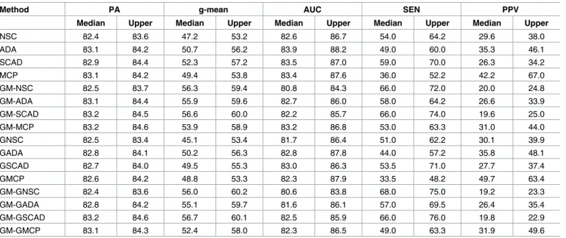
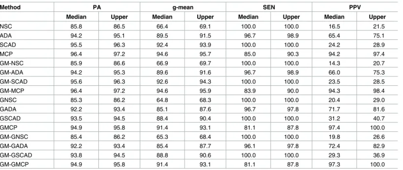
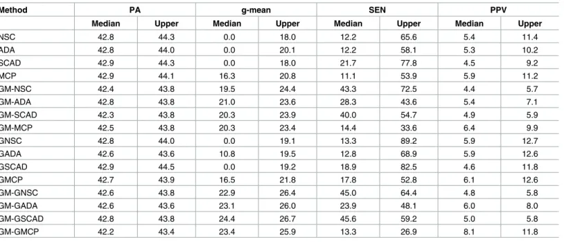
Simulation results for the three-class scenario have been presented in Tables5,6,7and8. Unlike the two-class scenario, class sizes were always imbalanced. However, we considered dif-ferent values ofγ, which was the effect size of DE genes, and observed that our proposed meth-ods performed significantly better than NSC. When the effect size of DE genes was moderate

Table 3. Two groups with sparse block diagonal structure (ρ= 0.5) and class-imbalance (π1= 0.8).

NSC 84.5 85.3 48.4 52.8 93.4 94.4 66.0 74.0 18.4 23.7

ADA 84.5 85.3 47.9 52.8 93.2 94.3 58.0 64.0 23.1 33.8

SCAD 84.7 85.3 49.0 52.4 93.5 94.4 65.0 71.2 19.6 22.8

MCP 83.8 84.5 43.6 49.4 92.1 94.0 41.5 56.0 38.1 55.1

GM-NSC 84.5 85.4 48.5 52.8 93.4 94.4 66.5 75.2 18.1 21.7

GM-ADA 84.5 85.3 48.1 52.8 93.2 94.3 58.0 64.0 23.1 32.2

GM-SCAD 84.7 85.3 49.0 52.4 93.5 94.4 65.5 72.0 19.4 22.7

GM-MCP 83.9 84.8 44.7 49.9 92.3 94.1 44.0 56.2 37.4 50.7

GNSC 84.4 85.4 48.2 52.8 93.3 94.5 65.5 73.2 19.0 24.6

GADA 84.4 85.3 47.9 52.1 93.5 94.5 56.0 67.0 26.3 32.1

GSCAD 84.3 85.3 47.6 52.0 93.4 94.4 64.0 69.0 20.6 24.0

GMCP 83.8 84.9 44.9 50.0 92.1 94.0 44.5 58.0 34.3 54.0

GM-GNSC 84.5 85.4 48.4 52.8 93.3 94.5 66.0 74.0 18.8 23.9

GM-GADA 84.4 85.3 47.9 52.1 93.5 94.5 56.5 67.0 26.3 31.5

GM-GSCAD 84.5 85.3 49.0 52.8 93.5 94.4 64.0 69.5 19.8 23.4

GM-GMCP 83.9 84.9 45.2 50.0 92.2 94.1 46.0 58.2 32.5 53.2

Table 4. Two groups with dense block diagonal structure (ρ= 0.9) and class-imbalance (π1= 0.8).

NSC 82.4 83.6 47.2 53.2 82.6 86.7 54.0 64.2 29.6 38.0

ADA 83.1 84.2 50.7 56.2 83.9 88.2 49.0 60.0 35.3 46.1

SCAD 82.9 84.4 52.3 57.2 83.5 87.0 59.0 70.0 26.3 34.2

MCP 83.1 84.2 49.4 53.8 83.4 87.6 36.0 52.2 42.2 67.0

GM-NSC 82.5 83.7 56.3 59.4 80.8 84.3 66.0 72.0 20.0 24.8

GM-ADA 83.1 84.4 55.9 59.6 82.7 86.0 58.0 64.2 26.6 33.9

GM-SCAD 83.2 84.5 56.6 60.0 82.2 85.7 66.0 74.0 19.6 25.0

GM-MCP 83.2 84.6 53.9 58.9 83.2 86.8 53.0 63.3 31.0 44.0

GNSC 82.5 83.4 45.1 53.4 81.7 86.4 51.0 62.2 30.1 39.9

GADA 82.8 84.1 50.2 56.3 82.8 87.8 44.0 57.2 35.8 48.1

GSCAD 82.7 84.0 49.5 55.3 83.0 86.3 53.5 71.0 27.7 37.4

GMCP 82.6 84.2 48.8 53.3 82.3 87.9 33.5 48.2 49.7 63.4

GM-GNSC 82.4 83.6 56.0 60.2 80.6 83.8 68.0 75.0 19.2 23.3

GM-GADA 82.8 84.2 55.1 59.7 81.6 86.1 57.0 69.5 26.4 35.4

GM-GSCAD 83.2 84.6 56.7 60.1 82.5 85.9 66.0 76.0 19.8 22.9

GM-GMCP 83.1 84.3 52.4 58.0 82.3 86.5 49.0 63.3 31.9 49.6

(11)

(γ= 0.5), only the ALT-NSC had better PA and g-mean, but GEN-NSC and GM methods showed no improvement. Under the very small effect size, all the classifiers performed very similarly in terms of PA, but their performance varied with respect to g-mean. MCP had the highest g-mean, and the other penalty functions gave zero as the median quartile of g-mean. Secondly, GM significantly improved g-mean for all the penalty functions, and the amount of the improvement was greater when the genewise penalties were used for the sparse block matrix. Finally, gene selection was also improved by GM: SEN increased and PPV stayed at

Table 5. Three groups with class-imbalance (π1= 0.4,π2= 0.2,π3= 0.4), sparse block diagonal structure (ρ= 0.5) and moderate mean difference

(γ= 0.5).

Method PA g-mean SEN PPV

Median Upper Median Upper Median Upper Median Upper

NSC 85.8 86.5 66.4 69.1 100.0 100.0 16.5 21.5

ADA 94.2 95.1 89.5 91.5 96.7 98.9 65.4 75.1

SCAD 95.5 96.3 92.4 93.9 100.0 100.0 24.2 28.9

MCP 96.4 97.2 94.6 95.7 85.0 90.3 94.2 97.4

GM-NSC 85.9 86.6 66.9 69.7 100.0 100.0 14.3 20.7

GM-ADA 94.2 95.3 89.6 91.6 96.7 98.9 66.0 75.3

GM-SCAD 95.6 96.3 92.6 94.3 100.0 100.0 23.5 28.5

GM-MCP 96.4 97.2 94.6 95.9 83.9 90.0 94.3 98.4

GNSC 85.3 86.2 64.8 68.3 100.0 100.0 20.4 29.0

GADA 92.2 93.4 85.1 87.6 96.7 97.8 71.7 81.6

GSCAD 93.5 94.5 88.4 90.4 100.0 100.0 31.2 40.7

GMCP 94.9 95.8 91.4 93.1 81.1 87.8 97.4 100.0

GM-GNSC 85.4 86.2 65.3 68.4 100.0 100.0 19.8 26.6

GM-GADA 92.2 93.4 85.4 87.7 96.1 97.8 72.4 82.9

GM-GSCAD 93.8 94.5 88.8 90.6 100.0 100.0 29.3 36.9

GM-GMCP 94.9 95.8 91.4 93.1 81.1 87.8 97.3 100.0

Table 6. Three groups with class-imbalance (π1= 0.4,π2= 0.2,π3= 0.4), dense block diagonal structure (ρ= 0.9) and moderate mean difference

(γ= 0.5).

NSC 84.6 85.5 62.6 67.5 98.9 100.0 28.7 36.7

ADA 92.5 93.6 86.3 88.5 94.4 96.7 74.6 84.1

SCAD 92.0 93.0 86.5 88.3 98.9 100.0 33.2 41.5

MCP 95.4 96.3 93.5 94.8 81.7 87.8 97.4 100.0

GM-NSC 84.8 85.6 68.2 70.1 100.0 100.0 16.5 21.4

GM-ADA 92.7 93.7 86.5 88.7 95.6 96.7 73.6 80.8

GM-SCAD 92.0 93.4 87.2 89.5 99.4 100.0 27.8 33.0

GM-MCP 95.3 96.3 93.5 94.8 81.7 86.9 97.4 100.0

GNSC 84.3 85.1 62.0 66.8 98.9 100.0 37.8 49.4

GADA 90.8 91.7 82.0 84.6 94.4 96.7 82.4 90.9

GSCAD 90.8 91.8 83.7 85.9 98.9 100.0 38.4 47.7

GMCP 94.1 94.9 90.3 91.9 78.3 86.7 98.6 100.0

GM-GNSC 84.2 85.1 66.0 68.1 100.0 100.0 20.6 30.2

GM-GADA 90.9 91.9 82.9 85.1 95.6 97.8 78.3 86.8

GM-GSCAD 90.9 91.9 84.0 86.3 98.9 100.0 34.0 43.0

GM-GMCP 94.2 94.9 90.3 91.6 78.3 86.9 98.6 100.0

(12)

almost the same value, compared to the corresponding methods based on the cross-validation prediction accuracy criterion.

Real data study

In this section, we applied conventional NSC and the proposed methods (ALT-NSC and GEN-NSC) to four real microarray data sets. The main characteristics of the four microarray data sets are presented inTable 9.

Table 7. Three groups with class-imbalance (π1= 0.4,π2= 0.2,π3= 0.4), sparse block diagonal structure (ρ= 0.5) and small mean difference

(γ= 0.1).

NSC 42.8 44.3 0.0 18.0 12.2 65.6 5.4 11.4

ADA 42.8 44.0 0.0 20.1 12.2 58.1 5.3 10.2

SCAD 42.9 44.3 0.0 18.0 21.7 77.8 4.5 9.2

MCP 42.9 44.1 16.3 20.8 11.1 53.9 5.9 11.2

GM-NSC 42.4 43.8 19.5 24.4 43.3 72.5 4.4 5.7

GM-ADA 42.8 43.8 21.0 23.6 28.3 43.6 5.4 7.1

GM-SCAD 42.3 43.8 20.3 23.9 40.0 54.7 4.9 5.9

GM-MCP 42.5 43.8 20.3 23.4 14.4 33.6 6.4 9.9

GNSC 42.8 44.0 0.0 19.1 13.3 89.2 5.9 12.7

GADA 42.6 43.6 10.8 19.5 12.8 68.9 5.9 12.6

GSCAD 42.9 44.5 0.0 19.2 18.9 82.5 4.6 11.8

GMCP 42.7 43.9 16.5 21.8 17.8 52.8 6.1 12.6

GM-GNSC 42.6 43.8 22.9 26.4 45.0 64.4 4.8 5.8

GM-GADA 42.6 43.6 23.1 26.0 23.9 48.1 6.0 8.0

GM-GSCAD 42.8 43.8 24.4 26.7 45.6 59.2 5.0 5.8

GM-GMCP 42.2 43.4 23.4 25.9 13.3 26.9 8.1 11.8

Table 8. Three groups with class-imbalance (π1= 0.4,π2= 0.2,π3= 0.4), dense block diagonal structure (ρ= 0.9) and small mean difference

(γ= 0.1).

NSC 40.5 41.8 0.0 27.5 5.6 25.8 6.7 17.9

ADA 40.7 41.9 0.0 28.3 5.0 30.0 6.3 17.2

SCAD 40.5 41.7 0.0 28.1 6.1 65.6 6.3 13.8

MCP 40.4 41.7 12.3 28.9 4.4 37.8 7.0 17.0

GM-NSC 38.7 40.1 31.2 33.0 61.7 86.9 4.4 5.2

GM-ADA 38.8 40.0 30.7 32.7 39.4 68.3 5.2 6.4

GM-SCAD 38.8 40.2 31.1 32.7 54.4 77.8 4.6 5.3

GM-MCP 39.3 40.3 29.5 31.9 17.8 50.0 6.2 9.1

GNSC 40.6 41.9 0.0 27.6 3.3 30.0 7.3 20.2

GADA 40.4 41.6 0.0 28.6 3.3 22.8 7.9 20.0

GSCAD 40.6 41.7 0.0 28.5 5.0 65.3 5.5 14.8

GMCP 40.1 41.2 21.4 30.0 5.0 26.1 7.2 17.3

GM-GNSC 38.6 39.5 30.8 32.4 55.6 81.4 4.6 5.8

GM-GADA 38.9 39.7 30.7 32.5 35.6 70.3 5.1 7.3

GM-GSCAD 38.6 39.5 31.3 32.8 48.3 75.6 4.7 5.5

GM-GMCP 38.9 39.9 30.5 32.2 25.0 53.6 6.0 9.6

(13)

The Gravier et al. [20] data set came from a breast cancer study that consists of 111 patients with no events and 57 patients with early metastasis after diagnosis. The Pomeroy et al. [21] data set is a CNS cancer study that consists of 10 medulloblastomas, 10 CNS AT/RTs (renal and extrarenal rhabdoid tumors), 8 supratentorial PNETs and 10 non-embryonal brain tumors (malignant glioma). The Yeoh et al. [22] data set is a acute lymphoblastic leukemia (ALL) study that consists of six types of pediatric ALL subtypes: 43 T-cell lineage ALL

(T-ALL), 27 E2A-PBX1, 79 TEL-AML1, 20 MLL rearrangements, 15 BCR-ABL, and 64 hyper-diploid karyotypes with more than 50 chromosomes (HK50). The Ramaswamy et al. [23] data set consists of 14 types of cancer samples as follows: 12 breast adenocarcinoma, 14 prostate adenocarcinoma, 12 lung adenocarcinoma, 12 colorectal adenocarcinoma, 22 lymphoma, 11 bladder transitional cell carcinoma, 10 melanoma, 10 uterine adenocarcinoma, 30 leukemia, 11 renal cell carcinoma, 11 pancreatic adenocarcinoma, 12 ovarian adenocarcinoma, 11 pleu-ral mesothelioma and 20 centpleu-ral nervous system.

We randomly split each data set into a training set and a test set with 33% of the data allo-cated to the test set. This process was iterated 100 times. We chose optimal tuning parameters (a,λ) as the values that give the maximum of 5-fold CV prediction accuracy or g-mean under Table 9. Characteristics of the real microarray data sets.

Author Reference Disease Class Gene Sample

Gravier et al. (2010) [20] Breast cancer 2 2905 168

Pomeroy et al. (2002) [21] CNS cancer 4 5597 38

Yeoh et al. (2002) [22] Leukemia 6 12625 248

Ramaswamy et al. (2001) [23] Cancer 14 16063 198

CNS: central nervous system. doi:10.1371/journal.pone.0171068.t009

Table 10. Gravier (2010) data set: Breast cancer study with 2 classes.

Method PA g-mean AUC N-sig

NSC 75.0 78.6 68.5 73.9 79.5 83.5 685 1176

ADA 75.0 78.6 68.5 73.9 79.9 83.3 550 1174

SCAD 75.0 78.6 69.3 73.9 79.9 83.3 928 1550

MCP 73.2 78.6 67.4 73.0 78.5 82.5 370 863

GM-NSC 75.0 78.6 70.5 75.7 80.9 83.8 660 968

GM-ADA 75.0 78.6 68.8 75.2 80.3 83.8 475 859

GM-SCAD 75.0 78.6 70.0 74.6 80.8 83.7 692 1196

GM-MCP 73.2 78.6 67.5 73.9 79.8 83.5 458 858

GNSC 75.0 78.6 70.4 74.1 80.0 83.5 720 1794

GADA 75.0 78.6 68.5 73.9 79.7 83.4 548 1198

GSCAD 75.0 78.6 68.5 73.9 80.0 83.2 908 1570

GMCP 73.2 78.6 67.5 72.2 78.4 82.9 435 1071

GM-GNSC 75.0 78.6 70.4 74.5 80.8 83.9 681 1396

GM-GADA 75.0 78.6 69.1 73.9 80.5 83.5 516 1007

GM-GSCAD 75.0 78.6 69.6 74.6 81.1 84.1 733 1191

GM-GMCP 75.0 78.6 68.5 73.5 79.7 83.3 480 848

(14)

the training data set. We compared prediction accuracy, g-mean, AUC (only for the Gravier data set) and the number of selected genes.

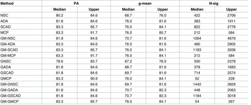
The Gravier data set is slightly imbalanced; the proportions of “no events” and “early metas-tasis” are 0.66 and 0.34. There was no improvement of PA, g-mean and AUC by the proposed methods, but using the alternative penalty functions reduced sig. MCP had the smallest N-sig (Table 10). The Pomeroy data set is balanced. ALT-NSC improved g-mean, but not PA, and reduced N-sig, with the exception of SCAD. GM did not improve either PA or g-mean. MCP performed the best with higher PA and g-mean and smaller N-sig compared to NSC. GMCP performed very similarly to MCP with slightly inferior prediction performance but much smaller N-sig (Table 11). The Yeoh data set is imbalanced. Like the Golub data set [24], the prediction was easy for this data set despite the large number of classes. PA and g-mean were not improved, but N-sig was reduced by the proposed methods. Both ALT-NSC and GEN-NSC reduced N-sig, with GMCP having the smallest N-sig. GMCP selected 418 genes, while NSC selected 1456 genes at the median quartile (Table 12). The Ramaswamy data set has a large number of classes, and, as a result, all the classifeirs had low g-mean values. All the MCP methods and GM-SCAD had positive g-mean values, but the other methods had zero as the 90% quantile of g-mean (Table 13).

Discussion

In this article, we proposed several variations of NSC that use alternative genewise shrinkages. We derived these methods using three penalized regression models that enjoy oracle proper-ties and have closed-form solutions under an orthonormal design. We also further modified these variants of NSC by adapting genewise penalty functions that use the correlations between the parameters belonging to the same gene, and the geometric mean approach for class-imbal-anced data. We showed that these methods have better performance than conventional NSC in terms of prediction accuracy, g-mean and gene selection through simuation and real data studies.

Table 11. Pomeroy (2002) data set: CNS study with 4 classes.

Method PA g-mean N-sig

Median Upper Median Upper Median Upper

NSC 80.2 84.6 68.7 76.0 422 2706

ADA 81.8 84.6 76.0 81.6 383 1911

SCAD 83.3 85.7 76.0 84.1 822 2776

MCP 83.3 91.7 76.0 85.7 212 584

GM-NSC 81.8 84.6 70.7 81.6 1264 4679

GM-ADA 83.3 84.6 76.0 81.6 480 2905

GM-SCAD 83.3 85.7 76.0 84.1 1183 3206

GM-MCP 83.3 91.7 76.0 84.1 212 584

GNSC 78.6 83.7 67.2 76.0 500 2378

GADA 81.8 84.6 68.7 81.6 378 1683

GSCAD 81.8 84.6 69.7 81.6 714 2574

GMCP 83.3 90.9 76.0 84.1 52 228

GM-GNSC 81.8 84.6 69.7 81.6 1442 3929

GM-GADA 81.8 84.6 70.7 82.3 448 2063

GM-GSCAD 81.8 84.6 70.7 82.3 1184 3018

GM-GMCP 83.3 85.7 76.0 84.1 54 267

(15)

We conducted simulation studies to evaluate the proposed methods. We used a block diag-onal covariacne matrix with the block being an auto-regresive structure with a paramterρ. Whenρis small, the block matrix becomes sparse, and thus it behaves like an identity matrix. Ohterwise, whenρis large, the block matrix becomes dense, and thus it behaves like a block exchageable matrix. We variedρ, the degree of class imbalance and the effect size of DE genes. Table 12. Yeoh (2002) data set: Leukemia study with 6 classes.

Median Upper Median Upper Median Upper

NSC 95.2 96.7 91.3 95.6 1456 2050

ADA 95.2 97.5 91.9 95.6 1044 2152

SCAD 95.2 96.4 92.1 94.8 1451 1991

MCP 95.2 96.4 93.9 95.5 1022 1454

GM-NSC 95.2 96.4 91.8 95.0 2168 3847

GM-ADA 95.2 97.5 94.0 95.6 2112 2310

GM-SCAD 95.2 96.4 92.2 94.8 1834 4072

GM-MCP 95.1 96.4 92.1 94.8 1454 2449

GNSC 96.3 96.4 93.9 95.6 690 1114

GADA 95.2 97.6 93.9 95.6 642 1041

GSCAD 96.3 97.6 94.0 95.6 990 1312

GMCP 96.4 97.6 93.5 95.6 418 496

GM-GNSC 95.2 96.4 93.9 95.6 931 1528

GM-GADA 95.2 96.7 94.0 95.6 820 1290

GM-GSCAD 96.3 96.4 93.5 95.3 1154 1998

GM-GMCP 96.4 97.6 94.4 95.6 484 911

Table 13. Ramaswamy (2001) data set: Cancer study with 14 classes.

Median Upper Median 90%* Median Upper

NSC 70.0 75.0 0.0 0.0 1570 4430

ADA 71.9 76.9 0.0 0.0 1346 3069

SCAD 70.6 75.4 0.0 0.0 2414 5233

MCP 72.3 77.4 0.0 62.1 1157 2566

GM-NSC 63.9 72.3 0.0 0.0 4610 16063

GM-ADA 69.7 76.9 0.0 0.0 2313 10264

GM-SCAD 68.7 75.8 0.0 55.6 6174 14779

GM-MCP 72.1 78.5 0.0 62.7 1575 4535

GNSC 68.7 73.8 0.0 0.0 396 1205

GADA 69.2 75.4 0.0 0.0 306 1042

GSCAD 68.2 73.6 0.0 0.0 539 5160

GMCP 70.3 77.0 0.0 0.0 206 578

GM-GNSC 18.5 68.7 0.0 0.0 6 16063

GM-GADA 60.3 71.6 0.0 0.0 466 16037

GM-GSCAD 60.9 70.4 0.0 0.0 3027 15757

GM-GMCP 69.2 75.5 0.0 58.3 234 3853

(16)

The proposed methods had better peformance in terms of prediction accuracy and gene selec-tion compared to NSC when the block matrix was dense and class was imbalanced. When the effect size was moderate, ALT-NSC methods performed well and among those MCP per-formed the best. When the effect size is small, GM method perper-formed well with the highest g-mean.

We applied the proposed methods to four real microarray data sets. The proposed methods improved the g-mean, but not the overall prediction accuracy, in the data sets we considered. When the number of classes was two (Gravier data set) or prediction was easy (Yeoh data set), only gene selection was improved by the alternative penalty functions. In the data set with the moderate number of classes (Pomeroy data set), g-mean was improved by the alternative pen-alty functions. When the data set had very large number of classes (Ramaswamy data set), using the genewise penalty functions reduced the performance.

In many applications, it is desirable to develop classifiers that use the smallest possible num-ber of genes. For example, one may wish to use an RT-PCR assay to discriminate between dif-ferent types of tumors or to determine the prognosis of a patient with a given tumor type. Such an assay will be prohibitively expensive if the expression levels of more than a handful of genes are needed. Thus, a classification method that produces comparable accuracy to another method using fewer genes would be considered superior in these situations. Hence, the fact that our proposed methods consistently use fewer genes than conventional NSC represents a significant advantage of our methods even if prediction accuracy is not always improved. MCP would be very useful in real applications becacuse they have shown to select the most reliable parsimonious gene set with competitive predictive accuracy.

Both simulation and real data studies showed that our proposed methods produced greater improvement compared to conventional NSC in the data sets with three or four clas-ses, but not in data sets with very large numbers of classes. When the number of classes is large, the sample size per class is usually small, and this affects the efficiency of shrunken mean estimators. By the virtue of the oracle property, ALT-NSC can produce more efficient estaimtes of the shrunken means, which yields better performance on both prediction and gene selection. Genewise shrinkages also improve the NSC classifier by combining the related genes in the same class, producing more accurate estimates when the size of the class is small (which commonly occurs when the number of classes is large). Clearly, the genewise penalty (GEN-NSC) shrinks a mean estimator toward zero faster than the non-genewise pen-alty (ALT-NSC), as shown in the simulations and the real data study. Appropriately fast shrinkage will be able to remove noisy genes effectively. However, one observes that when the number of classes is large, such as the Ramaswamy data set, the amount of shrinkage pro-duced by the genewise penalty is so large that NSC loses some prediction accuracy. Thus, applying GEN-NSC to data sets with too many classes may not be recommended when the objective is to maximize predictive accuracy (rather than minimize the number of selected genes).

(17)

Supporting information

S1 Rscript. R source code. This file contains the R functions that implement ALT-NSC and GEN-NSC.

(ZIP)

Acknowledgments

This work was supported by the National Research Foundation of Korea(NRF) grant funded by the Korea government(MSIP) (No. 2016943438). Eric Bair was partially supported by NIH/ NIDCR grant R03DE02359, NIH/NCATS grant UL1RR02574, and NIH/NIEHS grant P03ES01012.

Author Contributions

Conceptualization: BYC EB JWL.

Data curation: BYC.

Formal analysis: BYC.

Funding acquisition: JWL.

Investigation: BYC EB JWL.

Methodology: BYC EB JWL.

Project administration: JWL.

Resources: BYC.

Software: BYC.

Supervision: EB JWL.

Validation: EB JWL.

Visualization: BYC.

Writing – original draft: BYC.

Writing – review & editing: BYC EB JWL.

References

1. Tibshirani R, Hastie T, Narasimhan B, Chu G. Diagnosis of multiple cancer types by shrunken centroids of gene expression. PNAS. 2002; 99(10):6567–6572. doi:10.1073/pnas.082099299PMID:12011421 2. Tibshirani R, Hastie T, Narasimhan B, Chu G. Class prediction by nearest shrunken centroids, with

applications to dna microarrays. Stat Sci. 2003; 18(1):104–117. doi:10.1214/ss/1056397488

3. Wang S, Zhu J. Improved centroids estimation for the nearest shrunken centroid classifier. Bioinformat-ics. 2007; 23(8):972–979. doi:10.1093/bioinformatics/btm046PMID:17384429

4. Tibshirani R. Regression shrinkage and selection via the lasso. J R Stat Soc Series B Stat Methodol. 1996; 58(1): 267–288.

5. Guo Y, Hastie T, Tibshirani R. Regularized linear discriminant analysis and its application in microar-rays. Biostatistics. 2007; 8(1):86–100. doi:10.1093/biostatistics/kxj035PMID:16603682

6. Pang H, Tong T, Zhao H. Shrinkage-based diagonal discriminant analysis and its applications in high-dimensional data. Biometrics. 2007; 65:1021–1029. doi:10.1111/j.1541-0420.2009.01200.x 7. Shao J, Wang Y, Deng X, Wang S. Sparse linear discriminant analysis by thresholding for high

(18)

8. Mai Q, Zou H, Yuan M. A direct approach to sparse discriminant analysis in ultra-high dimensions. Bio-metrika 2012; 99(1):29–42. doi:10.1093/biomet/asr066

9. Blagus R, Lusa L. Improved shrunken centroid classifiers for high-dimensional class-imbalanced data. BMC Bioinformatics 2013; 14(64):1–13.

10. Fan J, Li R. Variable selection via nonconcave penalized likelihood and its oracle properties. JASA. 2001; 96(456):1348–1360. doi:10.1198/016214501753382273

11. Zou H. The adaptive lasso and its oracle properties. JASA. 2006; 101(476):1418–1429. doi:10.1198/ 016214506000000735

12. Zhang CH. Nearly unbiased variable selection under minimax concave penalty. Ann Stat. 2010; 38(2): 894–942. doi:10.1214/09-AOS729

13. Witten DM, Tibshirani R. A framework for feature selection in clustering. JASA. 2010; 105:713–726. doi: 10.1198/jasa.2010.tm09415PMID:20811510

14. Witten DM. Classification and clustering of sequencing data using a Poisson model. Ann Appl Stat. 2011; 5:2493–2518. doi:10.1214/11-AOAS493

15. Antoniadis A, Fan J. Regularization of wavelet approximations. JASA. 2001; 96:939–967. doi:10.1198/ 016214501753208942

16. Donoho DL, Johnstone JM. Ideal spatial adaptation by wavelet shrinkage. Biometrika. 1994; 81(3): 425–455. doi:10.1093/biomet/81.3.425

17. Breiman L. Better subset regression using the nonnegative garrote. Technometrics. 1995; 37(4): 373–384. doi:10.1080/00401706.1995.10484371

18. Gao HY, Bruce AG. Waveshrink with firm shrinkage. Stat Sinica. 1997; 7:855–874.

19. Dudoit S, Fridlyand J, Speed T. Comparison of discrimination methods for the classification of tumors using gene expression data. JASA. 2002; 97(457):77–87. doi:10.1198/016214502753479248 20. Gravier E, Pierron G, Vincent-Salomon A, Gruel N, Raynal V, Savignoni A, et al. A prognostic dna

sig-nature for T1T2 node-negative breast cancer patientsg. Genes Chromosomes Cancer. 2010; 49: 1125–1134. doi:10.1002/gcc.20820PMID:20842727

21. Pomeroy SL, Tamayo P, Gaasenbeek M, Sturla LM, Angelo M, McLaughlin ME, et al. Prediction of cen-tral nervous system embryonal tumour outcome based on gene expression. Nature. 2002; 415(6870): 436–442. doi:10.1038/415436aPMID:11807556

22. Yeoh E-J, Ross ME, Shurtleff SA, Williams WK, Patel D, Mahfouz R, et al. Classification, subtype dis-covery, and prediction of outcome in pediatric acute lymphoblastic leukemia by gene expression profil-ing. Cancer Cell. 2002; 1:133–143. doi:10.1016/S1535-6108(02)00032-6PMID:12086872

23. Ramaswamy S, Tamayo P, Rifkin R, Mukherjee S, Yeang CH, Angelo M, et al. Multiclass cancer diag-nosis using tumor gene expression signatures. PNAS. 2001; 98(26):15149–15154. doi:10.1073/pnas. 211566398PMID:11742071

24. Golub T, Slonim D, Tamayo P, Huard C, Gaasenbeek M, Mesirov J, et al. Molecular classification of cancer: Class discovery and class prediction by gene expression monitoring. Science. 1999; 286(5439):531–537. doi:10.1126/science.286.5439.531PMID:10521349