Invariant measures for continued fraction algorithms with finitely many digits

(1)

Invariant measures for continued fraction algorithms

with finitely many digits

Cor Kraaikamp

Delft University of Technology, EWI (DIAM), Mekelweg 4, 2628 CD Delft, the Netherlands, [email protected]

Niels Langeveld

Mathematical Institute, Leiden University, P.O. Box 9512, 2300 RA Leiden, The Netherlands, [email protected]

Abstract

In this paper we consider continued fraction (CF) expansions on intervals

differ-ent from [0,1]. For everyxin such interval we find a CF expansion with a finite

number of possible digits. Using the natural extension, the density of the invari-ant measure is obtained in a number of examples. In case this method does not

work, a Gauss-Kuzmin-L´evy based approximation method is used. Convergence

of this method follows from [1] but the speed of convergence remains unknown. For a lot of known densities the method gives a very good approximation in a

low number of iterations. Finally, a subfamily of the N-expansions is studied.

In particular, the entropy as a function of a parameterαis estimated forN = 2

andN= 36. Interesting behavior can be observed from numerical results.

Keywords: Continued fraction expansions, Gauss-Kuzmin-L´evy, entropy, natural extension, invariant measure

1. Introduction

In general, studies on continued fraction expansions focus on expansions for

which almost all x1 _{have an expansion with digits from an infinite alphabet.}

A classical example is the regular continued fraction [2, 3, 4]. An example of continued fraction expansions with only finitely many digits has been introduced in [5] by Joe Lehner, where the only possible digits are 1 and 2; see also [6]. More

recently, continued fractions have been investigated for which allxin a certain

interval have finitely many possible digits. In [7] the following 4-expansion has

1_{All ‘almost all}_x_{’ statements are wrt. Lebesgue measure.}

(2)

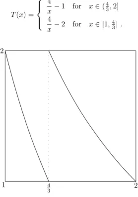
been (briefly) studied. LetT : [1,2]→[1,2] be defined as

T(x) =

    

4

x−1 for x∈( 4 3,2]

4

x−2 for x∈[1, 4 3].

(1)

1 2

2

4 3

..._... ... ..._...

... ..._...

..._... ... ..._...

... ..._...

..._... ..._...

..._... ... ..._...

..._... ..._...

... ..._...

..._... ..._...

..._... ...

..._... ..._...

..._... ...

..._... ..._...

..._... ...

Figure 1: The CF-mapT from (1).

By repeatedly using this map we find that everyx∈[1,2] has an infinite

con-tinued fraction expansion of the form

x= 4

d1+ 4

d2+. ..

(2)

with dn ∈ {1,2} for all n ≥ 1. The class of continued fractions algorithms

that give rise to digits from a finite alphabet is very large. In this paper we will give examples of such expansions and in Section 3 we will take a closer look at an interesting sub-family. Most of the examples will be a particular

case ofN-expansions (see [8, 9, 7]). Other examples are closely related and can

be found by combining the N-expansions with flipped expansions (cf. [10] for

(3)

suitable (from a computational point of view) for expansions with finitely many

different digits. This method is based on a Gauss-Kuzmin-L´evy theorem. For

greedyN-expansions this theorem is proved by Dan Lascu in [13]. The method

yields smoother results than by simulating in the classical way (looking at the histogram of the orbit of a typical point as described in Choe’s book [14], and used in his papers [12, 15]). We also give an example in which we do know the density and where we use this method to show its strength.

In Section 2 we will give the general form of the continued fraction maps we study in this paper. After that we give several examples of such maps and a way of finding the density of the invariant measure by using the natural extension. In Section 2.2 we will see how we simulated the densities in case we were not able to find them explicitly. In the last section we will consider a subfamily of

theN-expansions which can be parameterized by α∈(0,√N −1]. We study

the entropy as function ofα. We will do so mainly on a numerical basis. In the

past decades, it turned out to be very interesting to look at entropy of a family of continued fractions as a function of a parameter. In [16, 17, 18, 19, 20, 21, 22]

the entropy of Nakada’sα-expansions is studied. For example in [22] it is shown

that in any neighborhood of 0 you can always find an interval on which the entropy function is increasing, an interval on which the entropy function is decreasing and an interval on which this function is constant. In [18] it is shown that there is a countable set of open intervals on which the entropy function is monotonic. The union of these intervals has Lebesgue measure 1. As matching plays an important role in these papers we will take a glimpse at how matching works for our subfamily (see Section 3 for the definition and use of matching).

2. The general form of our maps

Throughout this paper we will look at continued fraction algorithms of the

following form. Fix an integer N ≥2 and let [a, b] be a subinterval of [0, N]

withb−a≥1. LetT : [a, b]→[a, b] be defined as

T(x) = ε(x)N

x −ε(x)d(x)

whereε(x) is either−1 or 1 depending onxandd(x) is a positive integer such

that T(x) ∈ [a, b]. Note that if b−a = 1 then there is exactly one positive

integer such that T(x) ∈ [a, b) if ε(x) is fixed. For N = 2 we find the family

that is studied in [10] and for ε(x) = 1 for all x we find the N-expansions

from [7]. Whenevera >0 this map can only have finitely many different digits.

This family is closely related to the (a, b)-continued fractions introduced and

studied by Svetlana Katok and Ilie Ugarcovici in [23, 24, 25]. For (a, b)-continued

fractionε(x) =−1 for all x∈[a, b] andN = 1. Also there are restrictions on

a, b. These are chosen such thata ≤ 0 ≤ b, b−a ≥1, −ab ≤ 1. The case

b−a = 1 was further studied by Carlo Carminati, Stefano Isola and Giulio

(4)

Note that this family is rather ‘large’. For the examples in the next sectionε(x) will be plus or minus one on fixed interval(s). In Section 3 other restrictions are imposed.

2.1. Two seemingly closely related examples and their natural extension

In [7], using the natural extension the invariant measure of the 4-expansion

mapT given in (1) was easily obtained. To (briefly) illustrate the method and

the kind of continued fraction algorithms we are interested in we consider a

slight variation of this continued fraction. Let ˜T : [1,2]→[1,2] be defined as

˜

T(x) =

     4

x−1 for x∈( 4 3,2]

5−4

x for x∈[1, 4 3],

(3)

i.e. we ‘flipped’ the mapT on the interval [1,4₃]; see also Figure 2.

1 4 3 2 2 ... ... ... ... ... ... ... ... ... ... ... ... ... ... ... ... ... ... ... ... ... ... ... ... ... ..._... ..._... ..._... ..._... ..._... ... ..._... ... ..._... ..._... ..._... ..._... ..._... ..._... ..._... ..._... ..._... ..._... ..._... ..._... ...

Figure 2: The CF map ˜T from (3).

Setting

ε1(x) =

1 forx∈(4₃,2]

−1 forx∈[1,4₃] and d1(x) =

1 forx∈(4₃,2]

5 forx∈[1,4₃] ,

we define εn(x) = ε1 Tn−1(x)

and dn(x) = d1 Tn−1(x)

. From T(x) =

ε1· 4

x−d1

, it follows that

x= 4

d1+ε1T(x) =. . .=

4

d1+

4ε1

d2+. .. +

4εn−1

dn+εnTn(x)

(5)

Taking finite truncations, we find the so called convergents

cn=

pn

qn

= 4

d1+ 4ε1

d2+. .. +4εn−1

dn

ofx. One can show that limn→∞cn=x; see [10] for further details. Therefore

we write

x= 4

d1+

4ε1

d2+. ..

, (5)

or in short hand notationx= [4/d1,4ε1/d2, . . .] orx= [d1, ε1/d2, . . .]4.

2.1.1. Using the natural extension to find the invariant measure

To demonstrate the method we will use ˜T from (3). The idea now is to build

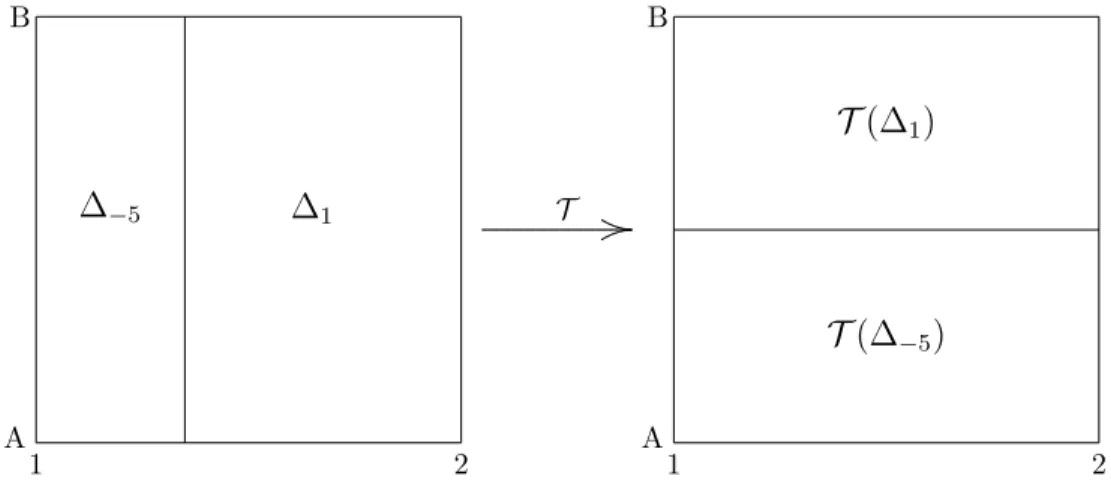
a two-dimensional system (the natural extension) (Ω = [1,2]×[A, B],T) which

is almost surely invertible and contains ([1,2],T˜) as a factor. In [7] it was shown

that a suitable candidate for the natural extension mapT is given by

T(x, y) =

˜

T(x), 4ε1(x) d1(x) +y

.

Now we choose A and B in such a way the system is indeed (almost surely)

... . . . . . . . . . .

T

A B

1 2 A

B

1 2

∆

1

∆

−5

T

(∆

1

)

T

(∆

−5

)

Figure 3: The suitable domain forT.

invertible. We define fundamental intervals ∆n = {(x, y) ∈Ω : d1(x) = n} if

ε= 1 and ∆−n ={(x, y)∈Ω :d1(x) =n} ifε=−1. When the fundamental

intervals fit exactly under the action ofT, the system is almost surely invertible;

(6)

choice here. It is shown in [7], that the density of the invariant measure (for the 2-dimensional system) is given by

f(x, y) =C 4

(4 +xy)2, for (x, y)∈Ω,

whereCis a normalizing constant (which is _log(3)1 in this example). Projecting

on the first coordinate yields the invariant measure for the 1-dimensional system

([1,2],T˜), with density

1 log(3)

₁ x+

1

4−x

, forx∈[1,2].

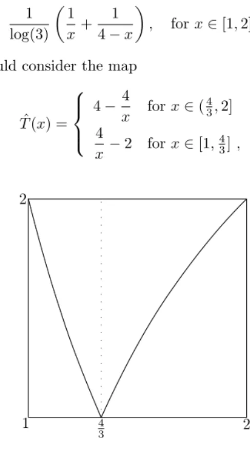
Note that if we would consider the map

ˆ

T(x) =

    

4−4

x forx∈( 4 3,2]

4

x−2 forx∈[1, 4 3],

(6)

1 2

2

4 3

..._... ... ..._...

... ..._...

..._... ..._...

..._... ... ..._...

..._... ..._...

..._... ..._......

... ...

Figure 4: The CF map ˆT from (6).

which is a ‘flipped version’ of the mapT from (1) where we flipped the branch

on the interval (4₃,2], we get another continued fraction of the form (5) but

now with digits dn ∈ {2,4}; see Figure 4. Our approach would give A =−2

andB =∞ which shows that the underlying dynamical system has a σ-finite

infinite measure with ‘density’f(x), given by

f(x) = 1

x+

1

2−x, forx∈[1,2].

(7)

will use an expansion given in [10]. Let ¯T(x) be defined as

¯

T(x) =

                     2

x−3 for x∈( 1 2,

4 7]

4−2

x for x∈( 4 7,

2 3]

2

x−2 for x∈( 2 3,

4 5]

3−2

x for x∈[ 4 5,1],

(7)

see Figure 5.

1 2 1 1 4 7 2 3 4 5 ... ... ... ... ... ... ... ... ... ... ... ... ... ... ... ... ... ... ... ... ... ... ... ... ... ... ... ... ... ... ... ... ..._... ..._... ... ..._... ..._... ... ..._... ..._... ... ..._... ..._... ... ..._... ... ..._... ... ..._... ... ..._... ... ..._... ... ..._... ... ..._... ..._... ..._... ... ... ... ... ... ... ... ... ... ... ... ... ... ... ... ... ... ... ... ... ... ... ... ... ... ... ... ... ... ... ... ... ... ... ... ... ... ... ... ..._... ..._... ..._... ..._... ..._... ..._... ..._... ..._... ..._... ..._... ..._... ..._... ... ..._... ..._... ..._... ..._... ..._... ..._... ..._... ..._... ..._... ..._...

Figure 5: An expansion map on [1 2,1]

When trying to construct the domain of the natural extension one quickly no-tices that ‘holes’ appear. This is not an entirely new phenomena in continued

fractions, it also appears in constructing the natural extension of Nakada’s α

-expansions whenα∈(0,√2−1); see [21]. One might hope that there are finitely

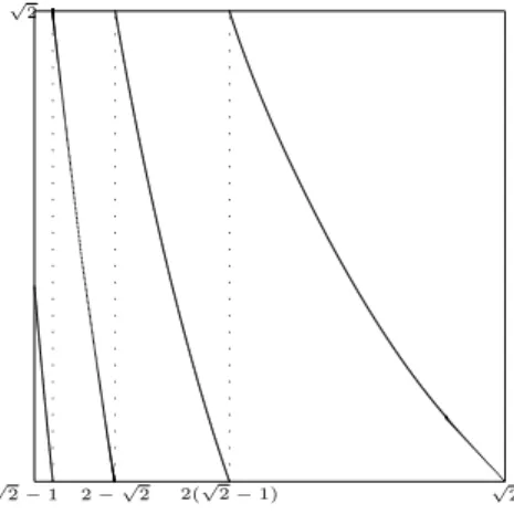
many holes, but a simulation of the domain indicates otherwise; see Figure 6. Although the method might still work in this case, it does not really seem to help us to find a description of the invariant density. In order to get an idea of the density we will use two different approaches. One will be based on the

Gauss-Kuzmin-L´evy Theorem. The other will be a more classical approach

(8)

Figure 6: A simulation of the domain of the natural extension for the map ¯T from (7).

2.2. Two different ways of approximating the density

The first way is based on the Gauss-Kuzmin-L´evy theorem. This theorem

states that for the regular continued fraction the Lebesgue measure of the

pre-images of a measurable setAwill converge to the Gauss measure.

λ T−n(A)

→µ(A) asn→ ∞.

This was stated as an hypothesis by Gauss in his mathematical diary in 1800 and proved by Kuzmin in 1928 who also obtained a bound on the speed of

convergence. Independently, L´evy proved the same theorem in 1929 but found a

sharper bound for the speed of convergence namely|λ(T−n₍_A₎₎₋_µ₍_A₎_|₌_O₍_qn₎

with 0< q <1 instead ofO(q√n_{) which is the bound Kuzmin found. There are}

many proofs of this theorem and refinements on the speed of convergence; see e.g. Khinchine’s book [3], or [27] for various refinements.

The idea for our method is to look at the pre-images of [1₂, z] for our map

¯

T from (7) and take the Lebesgue measure of the intervals found. Note that

in the first iteration you will find 2 intervals and after the first iteration the number of intervals found is multiplied by 4. Also the size of the intervals shrink relatively fast. Fortunately it seems that a low number of iterates (around 10) is already enough to give a good approximation; see Figure 8 where the theoretical density and its approximation are displayed and figure 7, where both methods of approximating are compared for a density we do not know the theoretical density.

The other way of finding an approximation is by iterating points and look at

the histogram of the orbits. The way we iterated is that we used a lot of

points and iterated them just a few times. To be more precise we iterated 2500 uniformly random points 20 times, repeated this process 400 times and took the average density of all points. Then we redid the process but instead of sampling uniformly we sampled from the previously found density (see also [28]) In Figure 7 we see both methods applied to our example.

The two methods give results that are relatively close but the approximation

found with the Gauss-Kuzmin-L´evy method is far more smooth. Since we do

not know the density we cannot compare the theoretical density with the

(9)

0.55 0.6 0.65 0.7 0.75 0.8 0.85 0.9 0.95 1 1.8

1.85 1.9 1.95 2 2.05 2.1 2.15 2.2 2.25

Figure 7: Approximations of the density of the invariant measure of ¯T(x) using the Gauss-Kuzmin-L´evy method (red) and the classical way (blue).

look how well this method performs in an example in which we know the

in-variant density explicitly. For the mapT from (1) we know the density which

was given in [7]. In Figure 8 we see a plot of both the theoretical density and

the approximation found by the Gauss-Kuzmin-L´evy method.

1.1 1.2 1.3 1.4 1.5 1.6 1.7 1.8 1.9 2 0.7

0.8 0.9 1 1.1 1.2 1.3 1.4

Figure 8: An approximation of the true density for the CF mapT from (1) and the true

T-invariant density.

The difference can barely be seen by the naked eye. If we look at the difference in 2-norm we get

Z 2

1

(f(x)−fˆ(x))2dx

12

= 1.1235∗10−5

(10)

3. A sub-family of the N-expansions

In this section we study a subfamily of the N-expansions (so ε(x) = 1 for

allxin the domain) with digits from a finite alphabet and an interval [α, β] as

domain. For our subfamily we want that it has finitely many digits. Furthermore

we would like that there is a unique digit such thatT(x)∈[α, β). This results

in α > 0 and β −α = 1. In this way the map is uniquely determined by

the domain. With these restrictions we define for α ∈ (0,√N −1] the map

Tα,N : [α, α+ 1]→[α, α+ 1] as

Tα,N=

N x −

_N x −α

.

Note that for all these expansions we have a finite number of digits sinceα >0.

Also note that this is the largest range in which we can choose αbecause for

α > √N −1 the digit would be 0 or less (see Section 3.2 for a calculation).

Simulations show that a lot of maps have an attractor smaller than [α, β]. When

N≥9 we find that ifα=√N−1 there is always an interval [c, d]([α, α+1] for

which theTα,N-invariant measure of [c, d] is zero. WheneverN >4 we have that

Tα,N always has 2 branches forα=

√

N−1. Calculations of these observations

are given in Section 3.2 in which we take a closer look on which sequences are

admissible for a given N and α. In Section 3.3 we study the behavior of the

entropy as a function ofαfor a fixedN.

The examples in [7] with ‘fixed range’ are all member of this kind of sub-family of

theN-expansions. Though, these examples are cases for which all the branches

of the mapping are full. In such case the natural extension can be easily build using the method described previously. If not all branches are full we can still make the natural extension in some cases. We will start this section with such case.

3.1. A 2-expansion withα=√2−1

LetT(x) : [√2−1,√2]→[√2−1,√2] be defined by

T(x) =

                    

2

x−1 for 2(

√

2−1)< x≤√2 2

x−2 for 2−

√

2< x≤2(√2−1) 2

x−3 for 1 7(6−2

√

2)< x≤2−√2 2

x−4 for

√

2−1≤x≤ 1

7(6−2

√

2).

(11)

√

2−1 √2

√

2

2(√2−1) 2−√2

..._... ..._... ..._... ..._... ..._... ..._... ..._... ..._... ..._... ..._... ..._... ..._... ..._... ... ..._... ..._... ..._... ... ..._... ..._... ..._... ..._... ..._... ..._... ... ..._... ..._... ... ..._... ..._... ... ..._... ... ..._... ... ..._... ..._... .... ..._... ... ..._... ..._... ... ..._... ... ..._... ..._... ..._... ... ..._... ... ..._... ... ..._... ..._... ..._... ..._... ..._... ..._... ..._... ... ..._... ..._... ... ..._... ... ...

Figure 9: A 2-expansion on the interval [√2−1,√2].

almost surely bijective on the domain (see Figure 10). We get the following

equations for the heightsA, B andC:

A= 2

4 +C , B=

2

3 +C andC=

2

1 +B .

... . . . . . . . . . . T A B C A B C

∆

1

∆

2 ∆3 ∆4

T

(∆

1

)

T

(∆

2

)

T(∆3)

T_(∆4)

(12)

This results inA= 1₂(√33−5),B= 1₆(√33−3) andC= 1₂(√33−3). We find the following invariant density up to a normalizing constant (which is given in Theorem 3.2)

f(x) =

  

√

33−3 4+(√33−3)x−

√

33−5

4+(√33−5)x for

√

2−1< x≤2(√2−1) √

33−3 4+(√33−3)x−

√

33−3

12+(√33−3)x for 2(

√

2−1)< x≤√2.

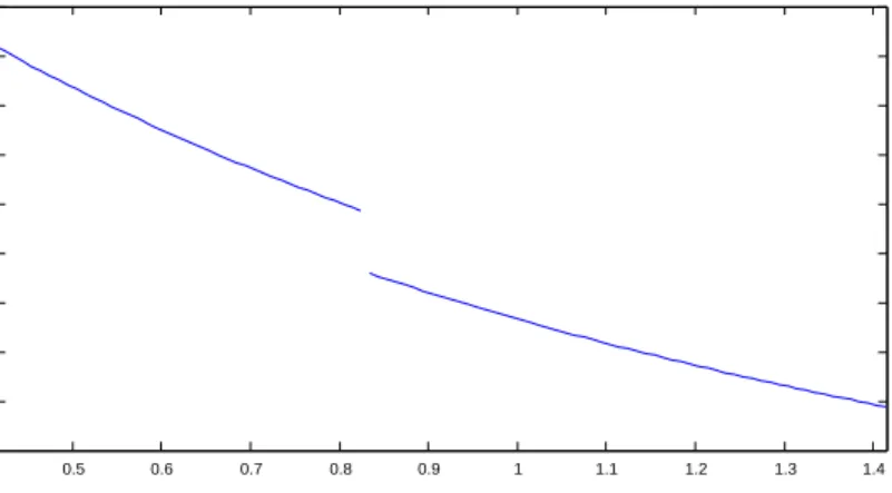
The graph of the density is given in Figure 11. In this case we were lucky. But

0.5 0.6 0.7 0.8 0.9 1 1.1 1.2 1.3 1.4 0.7

0.8 0.9 1 1.1 1.2 1.3 1.4 1.5

Figure 11: The density of the invariant measure for the 2-expansion on [√2−1,√2].

in general it seems to be very hard to construct the natural extension explicitly.

Still we can simulate the densities and calculate the entropy for a givenα. Also

for the 2-expansions we can extend the above result to allα∈[

√

33−5 2 ,

√

2−1];

see Theorem 3.1

3.2. Admissibility

In this section we look at how the alphabet is determined byαfor a fixedN.

It turns out that not all different sequences of such alphabet will occur in a con-tinued fraction expansion (or only finitely many times). This is a consequence of some cylinders having zero mass. The range of the first digits of a continued

fraction for givenαandN are easily described since the smallest digit will be

attained by the right end point of the domain largest digits will be attained by the left end point of the domain. Let

nmin=

_N α+ 1−α

and nmax=

_N α −α

.

Note thatnmin≤0 whenα >

√

N−1 and thereforeα=√N−1 is the largest

value for which we have positive digits. Furthermore the alphabet is given by

{nmin, . . . , nmax}. Now to see for which N we have that for α =

√

(13)

there are two branches we must check that nmax = 2. This happens when N

√

N−1−2∈[

√

N−1,√N]. We find 2 inequalities

N

√

N−1 −2≤

√

N (8)

and

√

N−1≤ √ N

N−1 −2. (9)

Inequality (8) gives 4≤N and inequality (9) givesN−1≤N. This yields that

for allN ≥4 we have two branches forα=√N−1. If N ≥9 we also have an

attractor which is strictly smaller than the entire interval for α=√N−1 as

the following calculation shows

Tα,N

[α, N

α+ 2]

=

α,N

α −2

Tα,N

[α,N

α −2]

=

α,N

α −2]∪[ N α

N−2α−1, α+ 1

Tα,N

[ N α

N−2α−1, α+ 1]

=

α,N

2₋₍₁₋₃_α₎_N₋₂_α

(α−1)N+ 2α

.

If we substituteαwith√N−1 and the following two inequalities hold we find

an attractor strict smaller than the interval [α, α+ 1];

N

√

N−1 −2<

N(√N−1)

N−2(√N−1) −1 (10)

N2−(4−3√N)N−2(√N−1)

(√N−2)N+ 2(√N−1) <

N

√

N−1 −2, (11)

yielding thatN ≥9. We take a closer look atN = 9 andα=√9−1 = 2. This

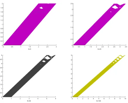
example is briefly discussed in [7] where it is stated that computer experiments suggest that the orbit of 2 never becomes periodic and therefore it is hard to find the natural extension explicitly. However, when simulating the natural extension, it seems that there are finitely many discontinuities; see Figure 12.

We can also simulate the density of the invariant measure; see Figure 13. Remark that cylinders with zero mass tells us which sequences are not appar-ent in any continued fraction of numbers outside the attractor and for those numbers not in the attractor these sequences only appear in the start of the continued fraction. We can describe which cylinders these are. The hole is

given by [2.5,2.6]. Now 2.5 = [1,1,1,1,1,1,1,1,2,1,1,1,1,1,1,2,2,1,1,1, . . .]9

and 2.6 = [1,1,1,1,1,1,1,2,1,1,1,1,1,1,2,2,1,1,1,1. . .]9. The boundary of a

cylinder ∆(a1, . . . , an) is given by [a1, . . . , an,1, r]9 and [a1, . . . , an,2, r]9 where

r is the expansion of 2. Now a cylinder is contained in [2.5,2.6] if 2.5 <

(14)

Figure 12: A simulation of the natural extension forN= 9 andα= 2.

2 2.1 2.2 2.3 2.4 2.5 2.6 2.7 2.8 2.9 3 0

0.2 0.4 0.6 0.8 1 1.2 1.4 1.6 1.8

Figure 13: A Simulation of the density forN = 9 andα= 2 using the Gauss-Kuzmin-L´evy method.

can have a clear description of the attractor and therefore for the admissible se-quences. Simulation shows us that there are a lot of different settings in which you find an attractor strictly smaller than the interval. In Figure 14

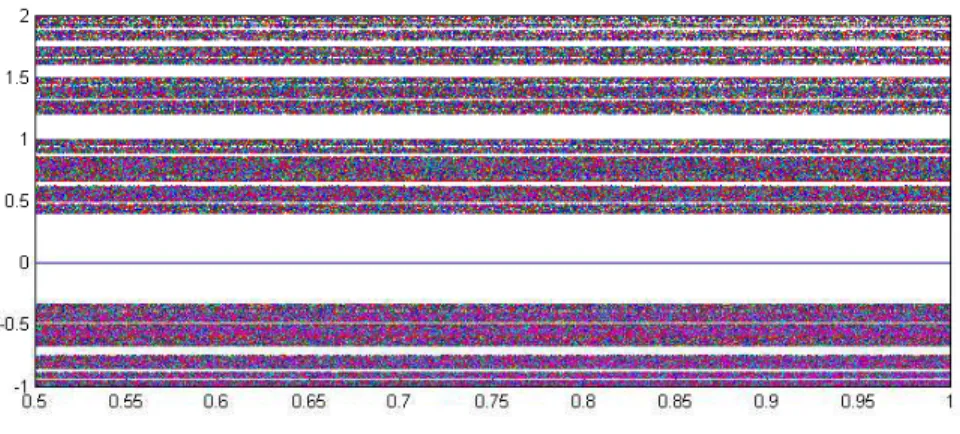
simula-tions for several values ofN are shown. On the y-axes αis given and on the

x-axes the attractor is plotted. For example, for N = 9 we see that for α= 1

there is no attractor strictly smaller than the interval. There is an attractor for

α= 1.8 and also for example forα= 2. The pattern seems to be rather regular.

Moreover, more ‘holes’ seem to appear for largeN and largeα.

3.3. Entropy

(15)

Figure 14: Attractors plotted for several values ofN.

it gives information about the speed of convergence for a typical point in that

system. Entropy as a function of a parameterαis widely studied for Nakada’s

α-expansions (see [17, 18, 19, 21, 22]). Also for the (a, b)-continued fractions the

entropy is studied [26]. A special interest goes to monotonicity which can be proven (for both cases) by using matching. It is shown that matching implies monotonicity and that matching holds almost everywhere. In this section we

look at entropy as a function ofα∈(0,√N−1] for a fixedN. For our family

it we do not know whether matching holds almost everywhere. In fact, it is

not even clear whether matching occurs for all N. Also, if matching implies

monotonicity is not clear. Certain conditions used to prove it in the case of

Nakadaα-expansions do not hold for our family and therefore we cannot mimic

the proof of [18]. Let us first give the definition of matching.

Definition 1 (Matching). We say matching holds for α if there is an K, M

such thatT_N,αK (α+ 1) =T_N,αM (α). The numbers K, M are called the matching exponents,K−M is called the matching index and an interval (c, d)such that for all α ∈ (c, d) we have the same matching exponents is called a matching interval.

Note that for Nakada’sα-expansions all rationals have a finite expansion and

thus match in 0 or before. For any rational in the domain a matching interval is found. For our family all rationals will have an infinite expansion. Since

for all α∈(0,√N −1) the expansion is infinite there are no values for which

(16)

it is hard to conclude it must hold in a neighborhood of α as well since we

cannot find an algebraic relation. The presence of the holes for someαmight

also lead to problems. The only reason to believe matching can help us to prove monotonicity is the fact that it works for related families and for specific choices

ofN andαwe can find matching where we can see the function is monotonic.

We will now discuss the 2α-expansions in detail. Moreover, we proof that the

entropy is constant forα∈

√

33−5 2 ,

√

2−1whenN = 2.

3.3.1. The entropy of2α-expansions

We start with an example for which there is no α such that we have an

attractor strictly smaller than the interval. Also, simulation indicates that there

seems to be a plateau in the neighborhood of√2−1. For this value we can

calculate the entropy since we have the density for this specific case ofα; see

Section 3.1 also see Figure 15 for a plot of the entropy function. When taking

Figure 15: Entropy as function ofαforN= 2.

a closer look at this plateau we found that on the interval [ √

33−5 2 ,

√

2−1] the

entropy is constant on this interval. The point √

33−5

2 is the point for which all

smallerα have that there are always 5 or more branches and for all larger α

there are always 4 branches. If we look at a simulation of the natural extension

it seems that for these values ofαwe can construct a natural extension. Indeed

this turned out to be the case (see Theorem 3.2). For √

33−5

2 we find matching

exponents (0,2) and for √2−1 we find matching exponents (0,1). Inside the

interval itself we find (3,3). As the value of the entropy, These values were first

found by simulation, in Theorem 3.1 we give a proof of this.

Theorem 3.1. Let N = 2, and let α ∈

√

33−5 2 ,

√

(17)

Proof. Note that the interval (α, α+ 1) has as natural partition{I1, I2, I3, I4}, where

I1= 2

α+ 2, α+ 1

, I2= 2

α+ 3, 2

α+ 2

i

, I3= 2

α+ 4, 2

α+ 3

i ,

and

I4= h

α, 2 α+ 4

i ,

where

T(x) = 2

x−d, ifx∈Id ford= 1,2,3,4.

An easy calculation shows that

T(α) =2−4α

α ∈I1,

(andT(α) = 2

α+2 when α=

√

2−1, and T(α) =α+ 1 when α=

√

33−5

2 ), so

that

T2(α) =3α−1

1−2α.

Furthermore, we have that

T(α+ 1) = 1−α

α+ 1 ∈I4,

(andT(α+ 1) =√2−1 whenα=√2−1;T(α+ 1) = _α₊₄2 whenα=

√

33−5 2 ),

so that

T2(α+ 1) = 6α−2

1−α.

Now let

K1=

√

33−5

2 ,

√

51−6

3

#

, K2=

√

51−6

3 ,

√

129−9

6

#

and

K3=

√

129−9

6 ,

√

2−1

! .

Forα∈K1 we have thatT2₍_α₎_∈_I3 _{and so}

T3(α) = 5−13α

3α−1

andT2₍_α_{+ 1)}_∈_I4 _{which results in}

T3(α+ 1) = 5−13α

3α−1 =T

(18)

Forα∈K2 we have thatT2(α)∈I2 and so

T3(α) = 4−10α

3α−1

andT2₍_α_{+ 1)}_∈_I3 _{which results in}

T3(α+ 1) = 4−10α

3α−1 =T

3₍_α₎_.

Forα∈K3 we have thatT2(α)∈I1 and so

T3(α) =3−7α

3α−1

andT2₍_α_{+ 1)}_∈_I

2 which results in

T3(α+ 1) = 3−7α

3α−1 =T

3

(α).

Earlier we thought we were just lucky finding the natural extension in case

N = 2 andα=√2−1. Note that from this natural extension we immediately

also have the caseN = 2,α=

√

33−5

2 ; just “invert” the time and exchange the

two coordinates in the natural extension we found forN = 2 and α=√2−1.

However, from Theorem 3.1 it immediately follows that we can also ‘build’ the

natural extension for everyα ∈

√

33−5 2 ,

√

2−1. Clearly, from Theorem 3.1

we see that we have three different cases.

Theorem 3.2. Forα∈

√

33−5 2 ,

√

2−1the natural extension can be build as in Figure 16. Moreover the invariant density is given by

f(x) = H( D

2 +Dx

1

(α,T(α+1))+

E

2 +Ex

1

(T(α+1),T2(α))+

F

2 +F x

1

(T2(α),α+1)

− A

2 +Ax1(α,T2(α+1))−

B

2 +Bx1(T2(α+1),T(α))−

C

2 +Cx1(T(α),α+1))

withA= √

33−5 2 , B=

√

2−1, C=

√

33−3 6 , D= 2

√

2−2, E=

√

33−3 2 , F =

√

2and

H−1= log ₃₂1(3 + 2√2)(7 +√33)(√33−5)2≈0.25the normalizing constant.

Proof. We guessed the shape of the domain of natural extension by studying a

simulation. For the map on this domain we usedT(x, y) =T(x), 2

d1(x)+y

.

Forα∈K1, we find the following equations:

A=₄₊2_E A=

√

33−5 2

B=₄₊2_D B =√2−1

C= ₃₊2_E C=

√

33−3 6

D= ₂₊2_A implying that D= 2√2−2

E=₁₊2_C E =

√

33−3 2

(19)

... . . . . . . . . .

T

A F

B C D E

α T(α+ 1) α+ 1 α α+ 1

T2 (α+ 1)T2 (α) T(α)

A F

B C D E

∆

1

∆

2

∆

3

∆

4

T

(∆

1

)

T

(∆

2

)

T(∆3)

T(∆4)

Figure 16: Ω andT(Ω) withα∈K1.

A similar picture emerges for α ∈ K2 and α ∈ K3. Moreover, you will find

the same set of equations and thus the same heights! Note that forα < 2₅ we

have T2₍_α₎_{< T}₍_α_{) for} _α₌ 2

5 we have T

2₍_α_{) =}_T₍_α_{) and for} _{α >} 2

5 we have

T2₍_α₎ _{> T}₍_α_{). When you integrate over the second coordinate you find the}

density given in the statement of the theorem. For the normalizing constant we have the following integral

H =

Z α+1

α

D

2 +Dx1(α,T(α+1)). . .− C

2 +Cx1(T(α),α+1)dx

= log

2 +DT(α+ 1)

2 +Dα

+. . .+ log

2 +CT(α)

2 +C(α+ 1)

= log

_{2 +}_DT₍_α_{+ 1)}

2 +Dα · · ·

2 +CT(α)

2 +C(α+ 1)

It seems thatH depends on αbut this is not the case. We will calculate one

(20)

log

_{2 +}_DT₍_α_{+ 1)}

2 +Dα

= log 2 + (2

√

2−2)T(α+ 1)

2 + (2√2−2)α

!

= log 2 + (2

√

2−2)1₁₊−α_α

2 + (2√2−2)α

!

= log 2(1 +α) + (2

√

2−2)(1−α)

2 + (2√2−2)α

!

+ log(1 +α)

= log √2

√

2(1 +α) +√2(√2−1)(1−α)

2 + (2√2−2)α

!

+ log(1 +α)

= log √22 + (2

√

2−2)α

2 + (2√2−2)α

!

+ log(1 +α)

= log(√2) + log(1 +α)

When calculating the second term one finds 1₄(√33−5)−log(1 +α) and so this

cancels the log(1 +α) term.

One might hope that when calculating the entropy using Rohlin’s formula, terms

will cancel as well. These integrals result inLi2 functions depending onαand

things are not so easy anymore. We provide a more elegant proof to show that

the entropy is constant on

√

33−5 2 ,

√

2−1and then calculate the entropy for

α=√2−1. We will use quilting introduced in [29]. Proposition 1 in this article

can be formulated (specific to our case) in the following way:

Proposition 3.3. Let(Tα,Ωα,Bα, µ)and(Tβ,Ωβ,Bβ, µ)be two dynamical

sys-tems as in our setting. Furthermore letD1= Ωα\Ωβ andA1= Ωα\Ωβ. If there

is ak∈Nsuch thatTαk(D1) =Tβk(A1)then the dynamical systems are

isomor-phic.

Since isomorphic systems have the same entropy it will give us the following corollary.

Corollary 3.4.ForN = 2the entropy function is constant on

√

33−5 2 ,

√

2−1

and the value is approximately1.14.

Proof. We show that for k = 3 we satisfy the condition in Proposition 3.3.

(21)

following regions (see Figure 17):

D1 = [α, β]×[A, D], D2 = [T(β), T(α)]×[B, C], D3 = [T2(β), T2(α)]×[E, F],

D4 = [T3(β), T3(α)]×

₂

3 +F,

2

3 +E

,

A1 = [α+ 1, β+ 1]×[C, F],

A2 = [T(β+ 1), T(α+ 1)]×[D, E],

A3 = [T2(β+ 1), T2(α+ 1)]×[A, B],

A4 = [T3(β+ 1), T3(α+ 1)]×

₂

4 +B,

2

4 +A

.

Note that since we have matching [T3(β), T3(α)] = [T3(β+ 1), T3(α+ 1)]. Now

2

3 +F =

2

3 +√2 =

2

4 +B =

2

4 +√2−1 ,

2

3 +E =

2

3 + √

33−3 2

= 2

4 +A =

2

4 + √

33−5 2

and so we findD4=A4.

... ... ..._... ... ... ... ..._... ... ... ... ..._... ... ... ... ..._... ... ... ... ..._... ... ... ... ..._... ... ... ... ..._... ... ... ... ..._... ... ... ... ..._... ... ... ... ..._... ... ... ... ..._... ... ... ... ..._... ... ... ... ..._... ... ... ... ..._... ... A F B C D E α

α+ 1

T(α+ 1)

T2 (α+ 1) _T₍_α₎

T2 (α)

β

β+ 1

T(β+ 1)

T2 (β+ 1) T(β)

T2 (β)

(22)

For the value of the entropy we use Rohlin’s formula forα=√2−1 (see [2, 4]);

h(T√

2−1) = Z

√

2

√

2−1

log|T0(x)|f(x)dx

= H

Z

√

2

√

2−1

(log(2)−2 log(x))f(x)dx

= log(2)−2H

Z

√

2

√

2−1

log(x)f(x)dx

= log(2)−2H

Z

√

2

√

2−1

log(x)((

√

33−3

4 + (√33−3)x−

√

33−5

4 + (√33−5)x)1

√

2−1,2(√2−1)

+(

√

33−3

4 + (√33−3)x−

√

33−3

12 + (√33−3)x)12(

√

2−1),√2)dx

= log(2)−2H((Li2(−x(

√

33−3)

4 ) + log(

x(√33−3)

4 + 1)

−Li2(−x( √

33−5)

4 ) + log(

x(√33−5)

4 + 1))|

2(√2−1)

√

2−1

+(Li2(−x(

√

33−3)

4 ) + log(

x(√33−3)

4 + 1)

−Li2(−x( √

33−5)

12 ) + log(

x(√33−5)

12 + 1))|

√

2 2(√2−1))

≈ 1.14.

By looking at the graph displayed in Figure 15 we can’t really find other match-ing exponents easily. To check for other matchmatch-ing exponents we can do the following. Suppose we are interested in finding a matching interval with

ex-ponents (n1, n2). We select a large number random points (say 10 000) from

(0,√N−1). Then we looked atTn1

α (α)−Tαn2(α+ 1) for these random points

and we checked to see whether it is very close to 0. Note that if an interval

was found this way with matching exponents (n1, n2) then we also find that

interval for (n1+ 1, n2+ 1). Table 1 shows which matching exponents we found.

This is very different from Nakada’sα-continued fractions where you can find

all possible matching exponents. The fact that we did not observe them does not mean they are not there. Maybe they are too small to observe using this method.

3.3.2. The entropy of36α-expansions

ForN ≥9 we expect different behavior due to the fact that for someαthere

is at least one subinterval on which the invariant measure is zero. If we pick

N = 36 we have a map with only full branches forα= 1,2,3. Figure 18 shows

the entropy as function of α. The stars indicate those values which we could

(23)

M\K 1 2 3 4 5 6 7 8 9 10

1 0 0 1 0 1 0 0 0 0 0

2 0 0 0 1 0 1 0 0 0 0

3 0 0 1 0 1 0 1 0 1 0

4 0 0 0 1 0 1 0 1 0 1

5 0 0 0 0 1 0 1 0 1 0

6 0 0 0 0 0 1 0 1 0 1

7 0 0 0 0 0 0 1 0 1 0

8 0 0 0 0 0 0 0 1 0 1

9 0 0 0 0 0 0 0 0 1 0

10 0 0 0 0 0 0 0 1 0 1

Table 1: observed matching exponents forN= 2: 1 if seen, 0 if not.

Figure 18: Entropy as function ofaforN= 36.

Clearly, we can observe plateaus but if we look at the matching exponents we

can observe that for all M, K ≤10 the only matching exponents we find are

(3,3),(4,4), . . .(10,10).

4. Conclusion

We have seen that the general form of the examples given yields a rather large family. In some examples we were able to construct the natural extension and therefore to find the invariant measure. In other examples this was not the case. There does not seem to be an easy rule which tells you when the

method will work and when it does not. The subfamily of theN-expansions we

studied is not new, but it has not been studied in this detail with finitely many

digits. Note that having the Gauss-Kuzmin-L´evy method for approximating the

densities allowed us to study the entropy much easier due to computation time. We have seen that matching is helpful to prove monotonicity even though we

did not mimic the proof forα-expansions. Motivated by similar results in the

case of Nakada’sα-expansions the following questions about entropy arise:

• For everyN ∈N≥2is there an interval in (0,

√

(24)

function is constant?

• For a fixedN ∈N≥2 for whichα∈(0,

√

N−1) do we have matching?

• Does matching holds on an open dense set? Does matching hold almost

everywhere?

• What is the influence of an attractor strictly smaller than the interval

[α, α+ 1] on the entropy?

References

[1] F. Schweiger, M. Waterman, Some remarks on Kuzmin’s theorem for F

-expansions, J. Number Theory 5 (1973) 123–131.

[2] K. Dajani, C. Kraaikamp, Ergodic theory of numbers, Vol. 29 of Carus Mathematical Monographs, Mathematical Association of America, Wash-ington, DC, 2002.

[3] M. Iosifescu, C. Kraaikamp, Metrical theory of continued fractions, Vol. 547 of Mathematics and its Applications, Kluwer Academic Publishers, Dordrecht, 2002.

[4] F. Schweiger, Continued Fractions and their Generalizations: A short

his-tory off-expansions, docentpress, 2016.

[5] J. Lehner, Semiregular continued fractions whose partial denominators are 1 or 2, in: The mathematical legacy of Wilhelm Magnus: groups, geometry and special functions (Brooklyn, NY, 1992), Vol. 169 of Contemp. Math., Amer. Math. Soc., Providence, RI, 1994, pp. 407–410.

[6] K. Dajani, C. Kraaikamp, “The mother of all continued fractions”, Colloq. Math. 84/85 (part 1) (2000) 109–123, dedicated to the memory of Anzelm Iwanik.

[7] K. Dajani, C. Kraaikamp, N. van der Wekken, Ergodicity of N-continued

fraction expansions, J. Number Theory 133 (9) (2013) 3183–3204.

[8] M. Anselm, S. H. Weintraub, A generalization of continued fractions, J. Number Theory 131 (12) (2011) 2442–2460.

[9] E. B. Burger, J. Gell-Redman, R. Kravitz, D. Walton, N. Yates, Shrinking the period lengths of continued fractions while still capturing convergents, J. Number Theory 128 (1) (2008) 144–153.

[10] N. D. S. Langeveld, Finding infintely many even or odd continued fractions by introducing a new family of maps, Master’s thesis (2015).

URLrepository.tudelft.nl

(25)

[12] G. H. Choe, Generalized continued fractions, Appl. Math. Comput. 109 (2-3) (2000) 287–299.

[13] D. Lascu, Dependence with complete connections and the gauss-kuzmin

theorem forn-continued fractions (2015).

[14] G. H. Choe, Computational ergodic theory, Vol. 13 of Algorithms and Com-putation in Mathematics, Springer-Verlag, Berlin, 2005.

[15] G. H. Choe, C. Kim, The Khintchine constants for generalized continued fractions, Appl. Math. Comput. 144 (2-3) (2003) 397–411.

[16] C. Bonanno, C. Carminati, S. Isola, G. Tiozzo, Dynamics of continued fractions and kneading sequences of unimodal maps, Discrete Contin. Dyn. Syst. 33 (4) (2013) 1313–1332.

[17] C. Carminati, S. Marmi, A. Profeti, G. Tiozzo, The entropy ofα-continued

fractions: numerical results, Nonlinearity 23 (10) (2010) 2429–2456.

[18] C. Carminati, G. Tiozzo, A canonical thickening of _Q and the entropy

of α-continued fraction transformations, Ergodic Theory Dynam. Systems

32 (4) (2012) 1249–1269.

[19] C. Carminati, G. Tiozzo, Tuning and plateaux for the entropy of α

-continued fractions, Nonlinearity 26 (4) (2013) 1049–1070.

[20] C. Kraaikamp, T. A. Schmidt, W. Steiner, Natural extensions and entropy

ofα-continued fractions, Nonlinearity 25 (8) (2012) 2207–2243.

[21] L. Luzzi, S. Marmi, On the entropy of Japanese continued fractions, Dis-crete Contin. Dyn. Syst. 20 (3) (2008) 673–711.

[22] H. Nakada, R. Natsui, The non-monotonicity of the entropy ofα-continued

fraction transformations, Nonlinearity 21 (6) (2008) 1207–1225.