Bayesian model-based methods for the analysis of DNA microarrays with survival, genetic, and sequence data

(1)

Bayesian Model-based Methods for the Analysis of

DNA Microarrays with Survival, Genetic, and

Sequence Data

Jonathan A. L. Gelfond

A dissertation submitted to the faculty of the University of North Carolina at Chapel Hill in partial fulfillment of the requirements for the degree of Doctor of Philosophy in the Department of Biostatistics, School of Public Health.

Chapel Hill 2007

Approved by:

Advisor: Joseph G. Ibrahim Co-advisor: Fei Zou

(2)

ABSTRACT

JONATHAN GELFOND:

Bayesian Model-based Methods for the Analysis of DNA Microarrays with Survival, Genetic, and Sequence Data

(Under the direction of Dr. Joseph G. Ibrahim)

DNA microarrays measure the expression of thousands of genes or DNA fragments

simultaneously in which probes have specific complementary hybridization. Gene

ex-pression or microarray data analysis problems have a prominent role in the biostatistics,

biological sciences, and clinical medicine. The first paper proposes a method for finding

associations between the survival time of the subjects and the gene expression of tumor

microarrays. Measurement error is known to bias the estimates for survival regression

coefficients, and this method minimizes bias. The latent variable model is shown to

detect associations between potentially important genes and survival in a breast cancer

dataset that conventional models did not detect, and the method is demonstrated to

have robustness to misspecification with simulated data. The second paper considers the

Expression Quantitative Trait Loci (eQTL) detection problem. An eQTL is a genetic

locus that influences gene expression, and the major challenges with this type of data are

multiple testing and computational issues. The proposed method extends the Mixture

(3)

the transcript location. The new technique exploits the fact that genetic markers are

more likely to influence transcripts that share the same location on the genome. The

third paper improves the analysis of Chromatin (Ch)-Immunoprecipitation (IP) (ChIP)

microarray data. ChIP-chip data analysis estimates the motif of specific Transcription

Factor Binding Sites (TFBSs) by comparing the IP DNA sample that is enriched for the

TFBS and a control sample of general genomic DNA. The probes on the ChIP-chip array

are uniformly spaced on the genome, and the probes that have relatively high intensity

in the IP sample will have corresponding sequences that are likely to contain the TFBS

motif. Present analytical methods use the array data to discover peaks or regions of IP

enrichment then analyze the sequences of these peaks in a separate procedure to

dis-cover the motif. The proposed model will integrate enrichment peak finding and motif

discovery through a Hidden Markov Model (HMM). Performance comparisons are made

(4)

ACKNOWLEDGMENTS

I would especially like to thank Dr. Joseph Ibrahim for his mentorship and his

research advice during the completion of this dissertation. Also, I would like to thank

Fei Zou and Mayetri Gupta for their important contributions and guidance as well as

the other members of my committee, Fred Wright and David Threadgill. I could not

have undertaken this dissertation without the generous support of the Howard Hughes

(5)

LIST OF TABLES

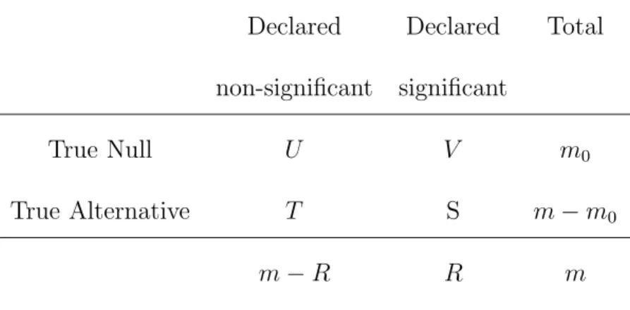
1 Possible outcomes for m hypotheses . . . 7

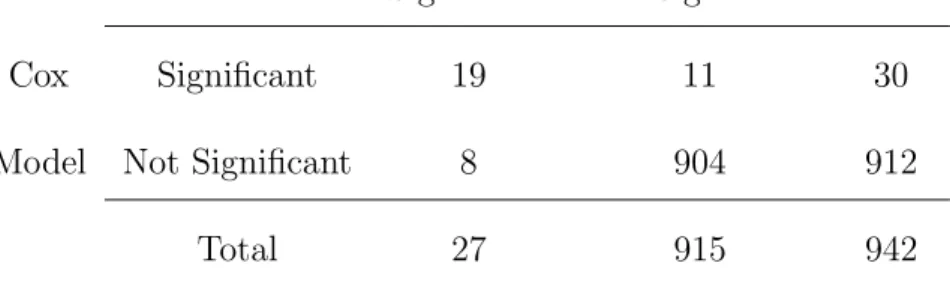
2 Comparison of Significant Genes . . . 42

3 Clinical Covariates Only Comparison . . . 43

4 Comparison of Significant Genes with Covariates . . . 44

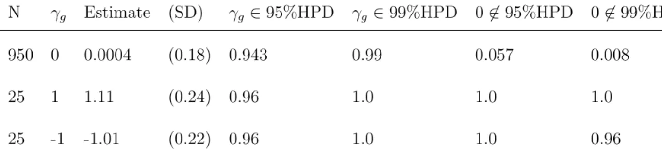
5 Operating Characteristics under True Model . . . 48

6 Operating Characteristics under Misspecified Model . . . 49

7 Simulated Data Parameter Estimates . . . 77

8 Simulated Data Parameter Estimates . . . 77

9 BXD Analysis Comparison of Parameter Estimates . . . 79

10 BXD Analysis Comparison of Differentially Expressed Genes . . . 80

11 Different Possible Probe Outcomes . . . 97

12 Simulations Based on Intensity Model Enrichment Estimates . . . 108

13 Simulations Based on TileMap Enrichment Estimates . . . 110

14 Parameter Estimates from IO and IS methods . . . 117

(9)

LIST OF FIGURES

1 Survival Curve for Breast Cancer Dataset . . . 22

2 Variance vs Mean Relationship with Model Fit Lines . . . 24

3 Trace Plots for Measurement Error Model . . . 40

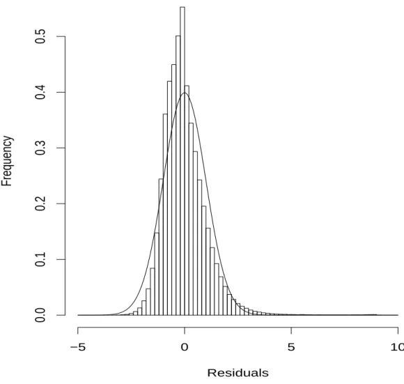
4 Scaled Residuals . . . 45

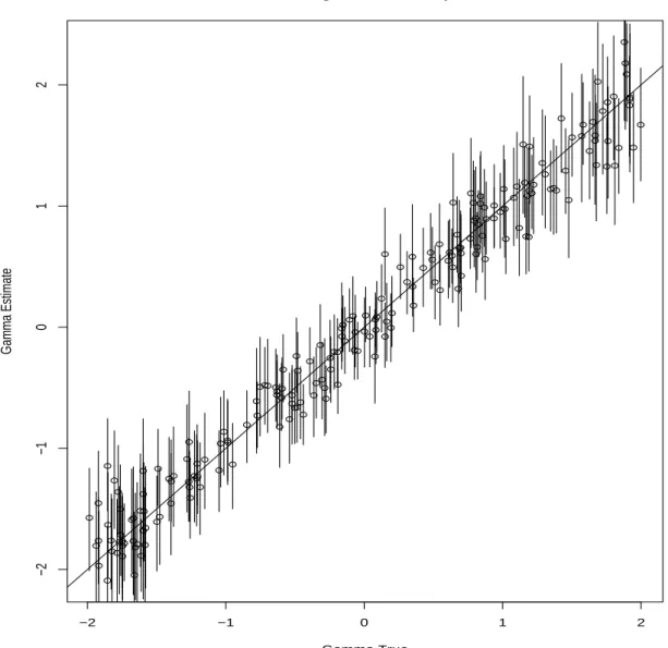
5 Estimation of Survival Regression Parameter . . . 47

6 Simulated Data Power Comparisons . . . 75

7 Simulated Data FDR Comparisons . . . 76

8 BXD Analysis Posterior distribution of eQTLs . . . 81

9 ChIP Process . . . 87

10 ChIP-chip Data Schematic . . . 90

11 ChIP-chip Data from Rap1 Experiment . . . 91

12 Likelihood Trace Plots for Accumulating Dictionary . . . 113

13 Selected Motif Logos of Accumulating Dictionary . . . 114

(10)

LIST OF ABBREVIATIONS

cDNA Complementary DNA

ChIP Chromatin Immunoprecipitation

DNA Deoxyribonucleic Acid

EM Expectation Maximization

FDR False Discovery Rate

HMM Hidden Markov Model

MCMC Markov Chain Monte Carlo

MLE Maximum Likelihood Estimate/Estimator

mRNA Messenger RNA

SNP Single Nucleotide Polymorphism

(11)

1 Introduction and Literature Review

Microarrays are quantitative assays that can measure the gene expression levels of

thou-sands of transcripts or millions of DNA fragments simultaneously. Since the mid 1990s,

this technology has provided a wealth of new biological and medical insights from the

discovery of the often subtle influences that experimental conditions can have on gene

expression to the recognition of previously unknown cancer subtypes. In the future,

one may expect that microarrays or similar technologies will provide insights into gene

networks, and that gene expression analysis will be used to guide clinical decisions on

chemotherapy to find optimal treatments and avoid unnecessary side effects.

The scientific potential of microarrays is enormous, and the statistical challenges of the

technology are nontrivial. First, there is the problem of multiple testing. Thousands or

even millions of dependent hypotheses can be tested in a single experiment. The simple

p-values and Bonferroni corrections have been enhanced by estimates of the false discovery

rates as a means of characterizing the certainties of inferences. Second, these hypotheses

are not made independently of one another. The genes do not work independently, and

the expression measurements of the genes share parameters between them that should

be modeled in order to utilize all of the information on the array. Third, microarrays are

indirect measurements that often have several components per transcript. An estimate

of the true expression level should be obtained that summarizes these components; these

(12)

difficulties such as normalization for experimental comparisons and outcome prediction

based on high dimensional data.

The dissertation is organized as follows. In Chapter 1, the scientific and statistical

fundamentals of microarrays are introduced. The first paper develops a measurement

error model for time-to-event data and tumor microarrays and is discussed in Chapter 2.

Chapter 3 presents the second paper and the analysis of genetics and microarrays. The

paper capitalizes on the relationship between genomic location and the genetic control

of transcription. The third paper is discussed in Chapter 4, and it concerns statistical

methods that use microarrays to discover transcription factor binding sites.

1.1 Fundamentals of Microarrays

Some biological and technological knowledge of how microarrays work is necessary for

the development and understanding of analytical methods. The biology that underlies

expression microarrays is often referred to as the “Central Dogma of Molecular Biology.”

For a review see Watson et al. (2004) or Stryer (1995). This is the principle that the

information coded in the nucleotide sequence of DNA is transcribed into mRNA which

is moved to the cytoplasm and translated into polypeptides that modulate and

enzy-matically promote most of the biochemical reactions in a cell. Gene expression is the

process of regulated transcription which is vital for cellular differentiation and function.

Microarrays are simultaneous measurements of this transcription process of thousands of

genes in a tissue or cell culture. Basically, a microarray is a snapshot quantification of

(13)

There are some specifics of polynucleotide molecules like DNA and RNA that are

vital to the self-reproductive properties of cells and to microarrays. DNA molecules are

sequences of nucleotide bases that are the purines adenosine and guanine and the

pyrim-idines thymine and cytosine. In RNA, the role of the purine thymine is replaced by uracil.

The polynucleotide chains of DNA and RNA will bind according to the hydrogen bonds of

their base sequence. The pyrimidines thymine, uracil have corresponding hydrogen bonds

with the purine adenine, and cytosine has corresponding hydrogen bonds with guanine.

These favorable configurations result in the complementary binding of adenine with

cy-tosine and uracil and the binding of guanine with cycy-tosine. Polynucleotide molecules will

preferentially bind to other nucleotides that have the complementary sequence, and this

process of one nucleotide binding to another is called hybridization. There are many

va-rieties of microarrays, but they all depend on the principle of specific hybridization. The

various mRNA of the cells are extracted through a technical process, but their sequences

remain specific to the gene from which they were transcribed in the cell. The cellular

extraction or sample of all of these mRNA is then labeled with either a fluorescent dye or

radioactive isotope that binds in a non-specific manner to the mRNA. On the microarray

slide is a spot or probe that contains the complementary sequence to a particular gene,

say “G1”. Sometimes multiple spots will represent the same gene, and these collection

of spots are called probe sets. When the sample makes contact with the slide, only the

“G1” mRNA will bind to the “G1” probes or spots because of the specific hybridization.

There may be tens of thousands of different probe sets each representing different genes

on an array. The fluorescent intensity or radioactivity of all of the probe sets can be

(14)

different probes, and a summary statistic of the intensity of light or radiation for each

probe is obtained by image analysis (Yang et al., 2001).

Two major classes of microarrays are the two color microarrays and the Affymetrix

oligonucleotide arrays. Some of the earliest microarrays used a two dye system to obtain

a relative quantification of mRNA (Cho et al., 1997). Two different samples of mRNA

are labeled with two different fluorescent dyes (e.g. red and green) and are hybridized

to the same array. The array probes are spots containing nucleotide sequences

comple-mentary to a specific gene. The ratio of red/green of the probe’s fluorescent intensity

is taken to be a relative measure of the mRNA levels corresponding to the biological

states of the two samples. Affymetrix high-density oligonucleotide arrays are synthesized

by a proprietary photolithography process that allows the synthesis of up to 105

differ-ent probes on the same array (Fodor et al., 1993; Lockhart et al., 1996). The probes

consist of short complementary sequences of length 25, and the probes are in perfect

match/mismatch pairs. The 13th _{nucleotide in a mismatch probe is not complementary} to the transcript sequence whereas the perfect match probes are entirely complementary

to the corresponding sequence. A probe set representing a gene will be about 10-20 pairs,

each complementary to a different part of the gene’s sequence.

1.2 Gene Expression Index

The Gene Expression Index (GEI) is the scalar valued summary statistic of the gene

ex-pression level based on the probe set data. For example, a probe in a two dye system has

(15)

and an experimental sample (red) (Pollack et al., 2002). The log-ratio of red/green

summarizes the two measurements by giving an estimate of the log of the ratio of the

concentrations in the two biological states. The motivation for using the log-ratio is

man-ifold. The ratio gives an easily interpretable comparison of the two concentrations and

may reduce variation from multiplicative noise that might be present in the measurement

variability of both the red and the green channels (Ideker et al., 2000; Rocke and Durbin,

2001). Taking the log acts to symmetrize the distribution of the ratio; the distribution of

the ratio is strictly positive and positively skewed. The log-ratio is not universal though,

sometimes the red and the green components are analyzed separately (Wolfinger et al.,

2001; Kerr et al., 2002).

In Affymetrix arrays, several different probes measure the presence of different

com-ponents of the gene’s sequence, and the models for the GEI are more complex. Early

studies used the average difference model (Lipshutz et al., 1999) as the GEI. Let PP M gij be the intensity measurement of the gth _gene’s_ith _{measurement of the} _jth _{perfect match} probe where j = 1, . . . , J, and let PM M

gij be the corresponding mismatch probe. The statistical model has the form

P_gijP M = νgj+θgi+P Mgij (1)

P_gijM M = νgj+M Mgij (2)

whereνgj is the common background effect, θi is the gene expression effect, andij is the random error. The average difference GEI is given by

ADgi = 1

J

J X

j=1

(16)

The motivation for the average difference model is the elimination ofν background

vari-ability, and the utilization of all probe data. However, there are some problems with

this model. It was seen that θgi could sometimes be negative which is problematic for estimates proportional to concentration. Also, the average difference model did not take

into account the reduced coefficient of variation for higher values. Li and Wong (2001)

proposed a model that had parameters that reflected the various probe sensitivities to

their target. The model is as follows

P_gijP M = νgj+αgjθgi+φgjθgi+P Mgij (4)

PgijM M = νgj+αgjθgi+M Mgij (5)

where φgi are the specific probe sensitivities, and αgi represent the probe sensitivities to non-specific binding. The φgj parameter had the constraint PJ_j₌₁φ2gj = J. Neverthe-less, Li and Wong showed that their model could give improved GEIs that would more

accurately detect differential expression in different biological states. Since the Li and

Wong model, there have been many competing models that give GEIs for Affymetrix

data such as Robust Microarray Analysis (Irizarry et al., 2003) and a mixed model

ap-proach of Hsieh et al. (2003). Both of these methods use a transformation of the intensity

measurements.

1.3 Microarrays and Multiple Testing

The types of hypotheses most common are those that test for the existence of an

as-sociation between a gene’s expression and the biological states of the collected sample.

(17)

Table 1: Possible outcomes in testing m hypotheses

Declared Declared Total

non-significant significant

True Null U V m0

True Alternative T S m−m0

m−R R m

(Cho et al., 1997; MacAlpine and Bell, 2005), irradiation exposure (Tusher et al., 2001;

Snyder and Morgan, 2004; Burns and El-Deiry, 2003), exposure to various compounds

(Bartosiewicz et al., 2001; Lobenhofer et al., 2004; Shultz et al., 2001), and survival times

(Hastie et al., 2000; Beer et al., 2002; Vijver et al., 2002). In these studies, there are

thousands of hypotheses because there are thousands of genes. We will refer to these

hypotheses asHi whereirepresents the gene identification number, andHi = 0 when the gene is under the null (no association), andHi = 1 when the gene is under the alternative (association). Classical methods generally focused on the development of testing

proce-dures that controlled the type I error rate for one or a few tests of hypotheses (Lehmann,

2005). New testing procedures were developed to increase the power of inferences in this

setting. Benjamini and Hochberg (1995) introduced the False Discovery Rate (FDR)

approach with the following Table 1.

The quantity m0

m is the proportion of hypotheses that are truly null, and it is often called π0. The family-wise error rate (FWER) is defined to be

(18)

FWER is the probability that there was at least one rejection of a null hypothesis or

false discovery. If the truth concerning the m hypotheses was known such that the table

could be constructed then the FDR would be given by

FDR = I[R >0]V

R =I[R >0] V

V +S. (7)

Since the truth concerning these hypotheses is not known, the FDR was defined to be

FDR = E

V

R|R >0

P{R >0} (8)

where V_R = 0 when R = 0. There is a closely rated concept of the positive false discovery rate pFDR = E[V_R|R > 0], but for microarray analyses P{R > 0} ≈ 1 so that FDR ≈

pFDR. A simple interpretation of the FDR is the expected proportion of false discoveries

in the set that is rejected. As Ge et al. (2003) point out,

FDR≤pFDR≤FWER. (9)

The above inequality is readily shown by writing the quantities as expectations and

illustrates the utility of the FDR to avoid the excessive strictness of controlling the

FWER. Biologists and clinicians are less concerned about the probability of making a

single false discovery (FWER) than in finding a set of genes that has a FDR that is

controlled in some sense.

The FWER, FDR or pFDR may be controlled in three ways, and these three ways

depend on the conditions under which these expectations are estimated. Strong control

is achieved when these expectations are bounded from above conditional on any set of

null hypotheses being true. Exact control is a bounding of the expectations under the

(19)

when the expectations are controlled under the complete null hypothesis which states

that all hypotheses are under the null. An important early result that Benjamini and

Hochberg (1995) proved for independent null hypotheses is that the FDR is controlled

in the strong sense under the following procedure. Order the p-values and let these be

P(1) ≤ P(2) ≤ · · · ≤ P(m). If one defines k to be the largest i such that P(i) ≤ _mi q∗ and

rejects the H(r) for r ∈ {1, . . . , k}, then the FDR will be less than π0q∗. They do not

estimate π0 so that they simply bound the FDR by q∗. Benjamini and Yekutieli (2001)

extended this type of procedure to handle arbitrary dependence in the test statistics.

This procedure is as follows. If one rejects k hypotheses when k is the largest ifor which

P(i)≤ Pmi

l=11/lq, then the FDR is no greater thanπ0q.

The Benjamini Hochberg (BH) procedure is an example of a stepwise procedure. A

stepwise procedure is one that involves using the rejection decision of other tests to

in-fluence the rejection of another. Specifically, the BH procedure is a step-up procedure

that starts at the least significant test (i.e. the largestp-value). Astep-downtest such as

the Westfall and Young (1993) procedure to control the FWER starts at the most

signif-icant test with the smallest p-value. These stepwise procedures are contrasted with the

single-step procedures like the Bonferroni, Sidak, minP and maxT p-value adjustments

(Ge et al., 2003). These are called single-step because the rejection decision of one test

does not involve the decisions concerning other tests.

Efron et al. (2001) and Storey (2003) utilize the connection between the FDR and

a Bayesian interpretation of the multiple testing problem. Efron et al. (2001) use an

empirical Bayes method to estimate the local false discovery rate that is the posterior

(20)

of the connection between the posterior probability and the FDR will be continued later.

The pFDR may be written as Storey (2002) did

pFDR(p) =P{Hi = 0|pi < p}=

π0P{pi < p|Hi = 0}

P{pi < p)}

(10)

with the exception that the p-value has been substituted for the test statistic. This

Bayesian construction leaves the problem of estimating the value of π0 which Storey

does by examining the distribution of thep-values. Storey argues that in an experiment

with π0 >0, the density of p-values over the interval [0,1] should become flat over some

subinterval [λ,1]. Given a choice of λ, an estimate ofπ0 is

ˆ

π0(λ) =

#{pi > λ}

(1−λ)m . (11)

This estimate of π0 is conservative (ˆπ0(λ) > π0) because some pi under the alternative could be greater than λ. The number of rejections R(p) is taken to be a function of the

p-value cutoff. He then estimates the pFDR as

\

pFDR_λ(p) = πˆ0(λ)p c

P r(P ≤p)[1−(1−p)m_]. (12)

In the above equation, the numerator ˆπ0(λ)pis an estimate of the probability of the false

positive, and the denominator is the product of estimates for the probability of rejection

givenp (P rc(P ≤p)) and the probability that R(p)>0 ([1−(1−p)m_{]). The probability} for rejection P rc(P ≤ p) is estimated by the observed rejection rate R(p)/m, and the probability that R(p) > 0 is conservatively estimated under that case that the null

hypotheses are independent. Storey et al. (2004) demonstrates that his method of pFDR

estimation provides strong control when the test statistics are independent or exhibit

(21)

V(p)/m0 and S(t)/(m−m0) converging almost surely as m → ∞. Weak dependence

holds for dependence in finite blocks and some other special cases, but it is not clear

that the correlation in expression data exhibits weak dependence. Specifically, there are

only a finite number of genes so that the meaning of asymptotic and continuity in the

empirical distribution cannot directly be applied.

Resampling methods like those of Yekutieli and Benjamini (1999) (YB) provide FDR

control under general dependence structure. Yekutieli and Benjamini (1999) use

resam-pling to control FDR in a similar manner as the Westfall and Young (1993) procedure

for controlling the FWER. Yekutieli correctly notes the FWER estimation through

re-sampling only requires that the null hypotheses rejectedV, but FDR estimation through

resampling requires that the number of true alternatives (S) is estimated giving

FDRest(p) =EV∗₍_p₎

V∗₍_p₎ V∗₍_p_{) + ˆ}_s₍_p₎

(13)

where p is the p-value threshold for significance. The YB procedure has an estimate of

S = ˆs that is negatively biased to ensure that the estimate of the FDR is conservative.

To this end, YB suggested using ˆs =mp. Reiner et al. (2003) compared the performance

in terms of power of the YB resampling method and the BH procedure. They concluded

that the YB resampling method provided small increases in power over the BH procedure.

Storey’s idea of estimatingπ0 based on the density of thep-values is similar in spirit to

the Beta-Uniform Mixture (BUM) method of Pounds and Morris (2003). In this method,

the density of the p-values is modeled by a BUM given by

f(p) =λ+ (1−λ)apa−1 (14)

(22)

given by ˆπ0 ≈ˆλ+ (1−λˆ)ˆa. The density ofp-valuesf is written as a mixture distribution

with uniform component ˆπ0I[p ∈ [0,1]] corresponding to the p-values under the null

which have cumulative distribution function F0(p) =p, and the alternative component

f(p)−πˆ0

1−πˆ0

(15)

which has cumulative density Fa(p). For any p-value cutoff τ, an upper bound of the FDR is given by

[

FDRub= πˆ0F0(τ) ˆ

π0F0(τ) + (1−πˆ0)Fa(τ)

. (16)

However, the BUM method does not model any dependence structure or address the

dependence theoretically. Broberg (2005) discusses the performance of the BUM method

as well as other methods under dependence, and found that the BUM method performs

reasonably well, but as dependence increases, the BUM method, like other methods, has

worsening performance.

There are a number of methods for estimating the FDR directly in terms of a posterior

probability. Efron et al. (2001) originally proposed the equivalence between local false

discovery rates and posterior probability, but Newton et al. (2001) developed a fully

Bayesian model for posterior probabilities involving a parametric hierarchical model for

two color microarray data. The model estimated the mixing proportion p of genes that

were differentially expressed using an Expectation Maximization (EM) (Dempster et al.,

1977) algorithm. The complete data involved an unobserved indicator variable zg that represented whether or not transcript g was differentially expressed. They advocated

using the first-order approximation of the posterior odds

odds = P(zg = 1|D)

P(zg = 0|D)

≈ pA(r, g)ˆp

p0(r, g)(1−pˆ)

(23)

where pA(r, g) and p0(r, g) are the parametric densities of the red (r) and green (g)

spot intensities under the alternative (differential expression) and the null respectively.

Kendziorski et al. (2003) extended this model to include different parametric assumptions.

Kendziorski used the posterior probability in an empirical Bayes framework as a decision

rule. These parametric models were extended to a semiparametric error model by Newton

et al. (2004a). Newton proposed using the average posterior probability to estimate the

FDR and control the FDR. He defined βg to be the posterior probability of the null hypothesis for gene g. The βg are then ranked from smallest to largest, and if βg is less than some κ, then the genes are identified as differentially expressed. One controls the

FDR in this framework by this estimate

[

FDR(κ) = P

gβgI[βg ≤κ] P

gI[βg ≤κ]

≤α. (18)

Clearly, FDR can be controlled by choosing an appropriate[ κ.

Considering the FDR as an average of posterior probabilities exposes a potential

problem in some FDR procedures like Storey’s q-value. This averaging quality of the

pFDR has been proved by Efron and Tibshirani (2002). In short, the FDR is problematic

because placing a bound on the average (FDR) of a set does not bound the members of

a set (posterior probabilities). Liao et al. (2004) point out the differences between the

posterior probabilities

P{Hi = 0|pi =p}=

π0

π0+ (1−π0)fa(p)

(19)

and Storey’s pFDR

P{Hi= 0|pi ≤p}=

π0p

π0p+ (1−π0)Fa(p)

(24)

where fa and Fa are the density and the cdf under the alternative. The right hand side in the above equation matches the FDRub in the BUM method. The difficulties with the

pFDR arise when considering inferences on specific genes. For example, it is possible

that the posterior probabilities for being under the null have a highly positively skewed

distribution, and the pFDR can be controlled but the gene of least significance could

have a posterior probabilities of being under the null equal to 0.99. Glonek and Soloman

(2003) give more examples of these poor decisions resulting in blindly controlling the

pFDR. This motivates the development of local FDR methods that approximate the

posterior probabilities such as Liao et al. (2004) and Efron (2004).

Other methods have been suggested to control the accuracy of multiple inferences

in microarray data. Versions of the negative predictive value for detecting differential

expression have been used by Liao et al. (2004) and Genovese and Wasserman (2002).

Also, Ibrahim et al. (2002) presented a parametric Bayesian model for modeling optimal

inferences concerning differential expression. This model includes correlation between the

genes as a form of dependency which was induced by the structure of the

hyperparame-ters. The ratio of the mean expression levels of different states for gene g is given by ξg. The posterior probabilityγg is defined asP(ξg>1|D), and a thresholdγ0 ∈[1₂,1] is then

selected such that geneg is differentially expressed if |γg−1₂| ≤γ0−1₂. The γ0 threshold

could then be set by using the L measure criterion. This model selection criterion was

developed by Ibrahim and Laud (1994), and it balances the posterior squared predictive

error and the posterior variance of the predictions for future observations. The optimal

model minimizes the L measure. In the gene expression model, several levels of γ0 were

(25)

be differentially expressed. This list is approximately optimal in terms of the L measure,

(26)

2 Microarrays and Survival Data

2.1 Cancer and Gene Expression

The first paper presents a method for finding associations between time-to-event data

and microarrays of tumors. Microarrays have been used to study cancer in many ways.

First, scientists saw in microarrays a technique for differentiating cancer types that

can-not be differentiated by other means. Microarrays are now capable of measuring every

gene in a cell giving a near complete picture of the transcriptome. The transcriptome

contains vast amount of information about tumors and can be used to differentiate

dif-ferent types of cancer. This process of classification of high-dimensional transcriptomes

into distinct subtypes is a statistical problem known as unsupervised classification or

clustering (Hastie et al., 2001). Methods of unsupervised classification include

hierar-chical clustering (Eisen et al., 2001), self-organizing maps (Tamayo et al., 1999), and

some more statistical methods like Parmigiani et al. (2002). Microarrays are not simply

a taxonomic tool, but the transcriptome gives biological insight as well (Golub et al.,

1999). Unsupervised clustering techniques can be used to find clusters of the genes,

and biologists recognize that genes within known pathways often are found within these

clusters (Golub et al., 1999; Perou et al., 2000). The discoveries of pathways and the

gene expression patterns involved in disease is a critical component of finding targets for

(27)

The transcriptomes of tumor samples have also been successfully used to predict

sur-vival for several different types of cancer including lung adenocarcinoma (Beer et al.,

2002), breast cancer (Sorlie et al., 2001; Sotiriou et al., 2003), hepatocellular

carci-noma(Lee et al., 2004), and leukemia (Chiaretti et al., 2004). The combination of survival

data and expression data has become an increasingly important and common analysis

problem. One of the fundamental difficulties in analysis of expression and survival data

is that the number of predictors (transcripts) is much larger than the number of

indepen-dent survival times. This leads to a noniindepen-dentifiability problem in estimating regression

parameters. Classical Principle Components Regression (PCR) involves using the

prin-ciple components of the data matrix as the linear predictors (Nguyen and Rocke, 2002).

The principle components with the smallest eigenvalues are discarded from analysis thus

reducing the dimension of the predictor matrix. However, Nguyen and Rocke (2002) have

shown that PCR performs poorly relative to the method of Partial Least Squares (PLS)

in predicting tumor classification based on expression profiles, but PLS is not optimal

in any reasonable way as shown by Butler and Denham (2000). The poor performance

of PCR is not surprising because principle components are an orthogonal decomposition

of the total variation of only the predictor matrix, and they are not necessarily

associ-ated with the variational patterns correlassoci-ated with survival. For example, the application

of unsupervised clustering techniques to tumor data can lead to classes that are not

associated with survival as seen by Bair and Tibshirani (2004).

Several strategies have been developed for predicting survival based on expression

data, and most of them used supervised methods of classification. Supervised

(28)

transcriptomes) are known in advance of the model construction (Hastie et al., 2001).

This is contrasted to unsupervised clustering methods like those that look for previously

unknown classes in the data. Naturally, survival times are continuous and censored in

nature, so forming discrete classes is often arbitrary. If these classes are treated as known,

then the stochastic properties are ignored which can lead to overfitting (Bair and

Tib-shirani, 2004). Nevertheless, there exist many mathematical techniques for supervised

classification such as neural networks (Wei et al., 2005), support vector machines (Lee

et al., 2003), and penalized logistic regression (Shen and Tan, 2005) that have been

ap-plied to tumor gene expression. Hastie et al. (2000) developed a “gene shaving” procedure

that is related to principle components analysis and takes advantage of the survival times

in order to find clusters of genes that are associated with survival. Gene shaving

accom-plished this by selecting genes into clusters by a balance of both their associations with

survival as well as correlations with other genes. There are several tuning parameters

that must be predetermined in the gene shaving method including the balance parameter

that determines the degree to which survival data influences the principle components in

the predictor matrix. Bair and Tibshirani (2004) created a semi-supervised method for

predicting survival in which only genes most associated with survival were included in a

reduced predictor matrix. The reduced predictor matrix was then decomposed into

prin-ciple components that are used in a predictive model. It is important to notice that the

univariate associations with gene expression play a vital role in some of these supervised

methods. In the first paper of the proposal, methods are developed for improving the

joint modeling of gene expression and survival that take into account the measurement

(29)

2.2 Measurement Error Models

The measurement error of microarrays is often not modeled directly by methods that

link gene expression and survival. Ideally, one would like to consider the variability

due to microarray measurement error when making inferences because microarrays have

significant amounts of assay noise (Yang et al., 2002). The presence of noise is obvious in

the case of assay replication, but assay noise can be confounded with biological variation

depending on experimental design. In the case where the biological states are finite (i.e.

treatment and control), there is often biological and technical replication of the states.

The assay noise in the presence of biological or technical replication is accounted for

by estimating the variance within replicates in the manner of t-statistics (Dudoit et al.,

2002). No two tumors constitute the same biological state. Unless the same tumor is

assayed more than once, the assay noise will be confounded with biological variation

between tumors. The analysis of noise in the absence of either biological or technical

replication is not straightforward, but it is of interest to account for the effects of assay

noise when dealing with time-to-event data. It is a well known phenomena that failure to

account for measurement error in covariates results in asymptotic bias of the estimated

effect toward the null (Prentice, 1982; Nakamura, 1992). This gives us motivation to

develop a model that includes assay noise and avoids biased inference. Tadesse et al.

(2005) have recently shown how inferences concerning microarrays and survival can be

affected by not accounting for measurement error in Affymetrix microarrays, and we

would like to build a similar model for cDNA microarray data.

(30)

mea-surement error in cDNA microarray experiments on the assessment of associations

be-tween gene expression and time-to-event data. We present a Bayesian hierarchical latent

variable model linked with a piecewise constant proportional hazards model for the

time-to-event data. The latent variable corresponds to the Gene Expression Index, and the

hazard function is conditional upon this latent GEI. The model is shown to have

favor-able properties such as robustness to misspecification and GEIs that do not explicitly

depend on platform specific parameters. Platform specific parameters include the

sensi-tivity of the red probe compared to the green probe and the reference sample. We apply

the model to a particular breast cancer experiment that previously demonstrated novel

subtypes of breast cancer based on gene expression profiles. The time-to-event of interest

is time-to-death due to disease.

Characterizing the association between time-to-event data and gene expression is

similar to the differential expression problem because event data constitutes a biological

state, although the state is complex in that the state space is censored and infinite. The

broader problem of differential expression requires that the gene expression for a

partic-ular gene on an array is measured or computed. The aforementioned value of a gene’s

expression is often referred to as the gene expression index (GEI) (Li and Wong, 2001).

The GEI is computed in numerous ways depending on the type of array and the model

used. The probes or spots on an individual array have complementary subsequences

highly specific to the corresponding gene’s RNA in the samples. The proposed model

extends the additive error-in-variable survival model for Affymetrix data of Tadesse et al.

(2005) to two color microarrays with correlated multiplicative errors. The error model

(31)

analyses are performed, and the model is applied to a breast cancer study dataset.

2.3 The Data Structure

The data analyzed were obtained from experiments performed on breast cancer samples

with similar types of cDNA microarrays. There were a total of 85 microarrays of tumor

(78), normal tissue (4), and other tissue (3) from 84 individuals, but clinical information

was available from only 77 of the individuals who corresponded to tumors. Of these 77

individuals, 75 had time-to-event data available. This subset of the data is the focus of

the paper. There were six batches of microarrays, some arrays having 24k probes and

others having 8k probes. A common subset of 7,938 probes were selected. In the green

channel, one of three batches of standardized reference were used. The red channel for

each array consisted of the 75 tumor samples. It has been reported that the differences in

the array type and the batch effect due to reference add some variability to the analysis

(Sorlie et al., 2001), but this noise is not considered here. The dataset is available from

the Stanford Microarray Database (http://genome-www.stanford.edu/microarray) . The

endpoint studied was time to death due to disease in months. Survival times were between

0 and 100 months (mean 35.43, median 30.0). Twenty-six of the 75 patients experienced

the event after time 0, A Kaplan-Meier curve of the 75 patients is shown in Figure 1.

2.4 The General Model

The goal is to characterize the association between gene expression of particular genes

(32)

0 20 40 60 80 100

0.0

0.2

0.4

0.6

0.8

1.0

Time in Months

Survival Proportion

Kaplan−Meier Plot of Data

(33)

measurement error model. The data is inherently trivariate in that the red and green

channels of any probe are potentially correlated with survival and jointly modeled. Some

notation will be introduced for this two color data. Each spot on the array will be

described asPgir which are vectors of length two whose indicesg,i andr refer to the gth gene and theith _{individual at the}_rth_{replicate respectively. The elements of}_P

girare Rgir and Ggir which are the red and green fluorescent measurements of the spot. Pgir may be

written as P robegir ≡Pgir =     Rgir Ggir    .

The measurement error model is adapted from one proposed by Ideker et al. (2000).

Ideker’s model consists of a bivariate normal error with an additive component and a

multiplicative component. The multiplicative component will be called the spot effect

(spot ≡ S). The spot effect is the motivation for taking the ratio of Rgir/Ggir. By dividing R by G, the general assumption is that the multiplicative error will cancel.

The additive component is related to the background effect (B). An examination of the

data reveals the relationship between the mean probe intensity and the variance of the

probe. Figure 2 shows the log of the sample variance plotted against log of the sample

mean in the green and red channels of our dataset. There appears to be a strong linear

relationship between log(probe mean) and log(probe variance).

Stating the model in equation form we have

Pgir=MgiSgir+Bgir, (21)

where

Sgir∼N2

        1 1    ,     σ2

mR ρmσmRσmG

(34)

5 6 7 8 9 10

10

12

14

16

18

20

Log(Probe Mean)

Log(Probe Variance)

a. Green Channel

5 6 7 8 9 10 11

10

12

14

16

18

20

Log(Probe Mean)

Log(Probe Variance)

b. Red Channel

(35)

Bgir∼N2         0 0    ,     σ2

aR ρaσaRσaG

ρaσaRσaG σ2aG        , and

Mgi=    

µRgi 0 0 µGgi

   .

The diagonal elements ofMgi are interpreted as the mean intensities for geneg and state

i since E[Pgir] = [µRgi µGgi]0, and this is what motivates the mean vector of     1 1     for

Sgir. The covariance parameters for the multiplicative error are σ2

mR,σ2mG, andρm which represent the variability due to a multiplicative effect in assay replication of biologically

identical samples. Similarly, the covariance parameters for the additive variability due

to replication areσ2

aR,σaG2 , and ρa.

There are other models for cDNA data with both additive and multiplicative

compo-nents. Rocke and Durbin (2001) suggest a log-normal multiplicative error with a normal

additive error. This model presents major computational challenges because Pgir does not have a standard distribution, and the likelihood cannot be written in closed form.

Rocke and Durbin (2001) suggest an iterative fitting procedure on different subsets of

genes for the additive and the multiplicative components separately. However, we do not

choose this model for three reasons. First, analysis of the residuals of the log transformed

data suggest that the log-transformation over-corrects for the relatively small amount of

skewness in the data. Second, the difficulty of dealing with a nonstandard distribution

adds to an already heavy computational burden. Third, we show in Section 2.6 that the

(36)

assump-tion are robust to this type of misspecificaassump-tion of the multiplicative error distribuassump-tion.

However, even the Ideker model is not identifiable unless there is technical replication

in both the red and green channels. In the dataset considered in this paper, we do not

have such replication except in a small number of duplicate probes on each array (about

180). An analysis of these probe measurements was performed on the green and the red

channels separately, and the estimates of σ2

mR and σ2mG were found to be approximately equal. With this justification, we set the constraint σ2

mR = σmG2 = σm2 for the purpose of model identifiability. Also, the variance parameters due to the additive components

(σ2

aR,σaG2 , andρa) were found to be very small relative to the multiplicative error, so we set them to zero. The parameters µRgi and µGgi are the means within a biological state. When a common reference is used,µGgibecomesµGgand it represents the mean intensity of the reference channel, and µRgi is the mean of the sample channel. In experiments with biological replication within a channel, the means of the intensities measured are

often considered to be derived from the same underlying population, so that µRgi =µRg for replicates within a biological state. We must account for the biological variability in

tumor samples, and thus we consider an additional hierarchical component to the model

and take µRgi =µRg(1 +βgi) The parameter βgi is the latent GEI and represents the ith tumor’s and the gth _{gene’s deviation from mean of that gene (}_µ_Rg). _β

gi is taken to be a truncated normal variable withβgi >−1 because βgi+ 1 is considered to be proportional to a concentration, and therefore, βgi+ 1 must be positive. The method of identifying the GEI as a latent variable is novel. It is well suited for tumor samples because it gives

a structure to the variation in a gene’s expression. The structure of the truncated normal

(37)

the mean. The model can be restated in another equivalent form.

Rgi = µRg(1 +βgi)Rgi (22)

Ggi = µGgGgi (23)

where

Sgi≡     Rgi Ggi    ∼         1 1    ,     σ2

m ρmσm2

ρmσm2 σm2         and

βgi ∼N{βgi>−1}(0, σ

2

bio).

We have a simple physical model that assumes that the intensity of a probe (P) is roughly

proportional to product of the concentration ([mRNA]) of the target mRNA in the sample

and the sensitivity of the probe (φ). In equation form we have P ≈ [mRNA]×φ. The physical model is motivated in part because of the Li and Wong model for Affymetrix

data which takes the following form for a single gene:

Pij=νj+θiφj+ij (24)

Here, Pij represents the ith measurement jth probe with sensitivity φj and background

νj. θi is the gene expression index and ij is a normally distributed error term. The difference between our model and models like that of Li and Wong is that the GEI of

individual i is not a random effect. That is, in the Li and Wong model, the biological

variation of GEI’s is not modeled explicitly. We extend the form of the Li and Wong

model to cDNA data here for the case of a standard reference in the green channel by

taking

(38)

where Φg =    

φRg 0 0 φGg

  

 and Θgir=    

[red]gi 0

0 [green]g    .

The parameters φRg and φGg are the platform specific sensitivities of the red and green channels respectively. The Θgi denotes a matrix whose diagonal elements [red]gi

and [green]g are the concentrations of RNA on the specified array. This model statement

is consistent with (21) if we let ΘgiΦg =Mgi and set Bgi = 0. The problem of gene by dye interaction occurs for some genes when the intensity of the red channel and the green

channel respond differently to the same concentration gradient. Using the language of

this model, gene by dye interaction can be stated as φRg 6= φGg. The connection with this model and the log-ratio can be seen by considering the special case that ρm = 1. The log-ratio is given by

ψgir ≡log(Rgir/Ggir) = log ((φRg/φGg)([red]gi/[green]g)). (26)

The three deficiencies ofψgircan be noticed. First, if the values in the red or green channel are negative, then the log-ratio cannot be computed, and this generates missing data

despite the clear informativeness of low values. Second, the platform specific parameters

of φRg and φGg are contained in the GEI. Third, the reference specific parameter µGg is also affecting the GEI, and these two problems complicate the interpretation and the cross

platform comparisons of the log-ratio. Now, consider the parameter βgi. The parameter can be stated in terms of the ratio of intensity parameters as βgi = (µRgi/µRg) −1. According model 29, µRgi =φRg[red]gi and µRg =φRg[redg] then,

βgi = (µRgi/µRg)−1 = ([redgi]/[red]g)−1. (27)

(39)

the reason that it is a function of the ratio of the mean intensities, and that ratio is not

dependent on the probe sensitivity or the reference channel.

The parameter βgi will also be linked to the following piecewise constant hazards survival model. This model divides the survival time axis intoJadjacent disjoint intervals

(s0, s1],(s1, s2], ...,(sJ−1, sJ] where 0 = s0 < sj < sj0 if (0 < j < j0) and j = 1, . . . J.

Within each interval is a constant baseline hazardh0(y) =λj when y∈(sj−1, sj]. We let

νi = 1 be the failure indicator for the ith individual (νi = 0 otherwise), and let δij = 1 if the ith _{individual was either censored or failed in the} _jth _{interval (}_δ

ij = 0 otherwise). The survival component contribution of the likelihood for the ith _{individual becomes}

f(yi|βgi, γc) = J Y

j=1

(λjexp(ηi))δijνiexp{−δij "

λj(yi−sj−1) +

j−1

X

k=1

λk(sk−sk−1)

#

exp(ηi)} (28)

where ηi = log(βgi+ 1)γg+Zi0γc is the linear predictor. Zi is the p×1 vector of clinical covariates for the ith _{individual, and} _γ

c is the corresponding p×1 vector of coefficients. Note thatβgi has been log transformed for comparisons with the log-ratio models.

In this paper, we consider only one gene’s (g =g0_{) association with survival at a time}

so βg0 refers to the vector of latent GEI’s for the g0(th) gene, but P refers to all probe

data, that is all of the red and green channel measurements. The model parameters are

Ω ={λj, βg0_i, γ0_g, γ_ck, µ_Rg, µ_Gg, σ_m, ρ_m, σ_Bg}.

(40)

by

L(Ω|D)∝

n Y i=1 G Y g=1 φ2    Pgi;

   

µRg(1 +βgi)

µGg    ,     µ2

Rgiσ2m ρmσm2µRgiµGg

ρmσ2mµRgiµGg µ2Ggσm2        

× φ{βgi>−1}(βgi; 0, σ

2 Bg) × J Y j=1

λje(log(βg0i+1)γg0+Ziγc)δijνi I[g=g0_]

×

"

exp{−δij "

λj(yi−sj−1) +

j−1

X

k=1

λk(sk−sk−1)

#

elog(βg0i+1)γg0+Ziγc_}

#I[g=g0_]

. (29)

where φ2() is the bivariate normal density, and φ{βgi>−1}() is the left truncated normal

density. Again, ηi = log(βg0_i + 1)γ_g0 +Z_iγ_c is the linear predictor for survival involving

only one gene (g0_{). Also,} _µ

gRi =µgR(1 +βgi) for convenience.

The likelihood has two parts. The first part will pertain to the measurement error

model, and the second part is the survival model. This dichotomy of the likelihood

motivates the two stage fitting procedure described in Section 2.4.2.

2.4.1 Priors

Bayesian models involve the specification of priors as well as the likelihood, therefore

the specification of priors will complete our model. We do not have information about

parameters from previous studies, and therefore we choose priors that are relatively

(41)

µ−_Rg1|µi, σµ2i ∼ N{µRg>0}(µim

−1

Rg, σ2µim

−2

Rg) [mRg = 1

ng ng

X

i=1

Rgi] (30)

µ−_Gg1|µi, σµ2i ∼ N{µGg>0}(µim

−1

Gg, σ

2

µim

−2

Gg) [mGg = 1

ng ng

X

i=1

Ggi] (31)

σ_m−2|αm, ωm ∼ gamma(αm, ωm) (32)

ρm ∼ Unif(0,1) (33)

σBg|αB, ωB ∼ gamma(αB, ωB) (34)

λj|α0, ω0 ∼ gamma(α0, ω0/λj−1)(λ0 = 1) (35)

γg0|σ_g2 ∼ N(0, σ_gene2 ) (36)

(37)

The gamma priors on the λj’s are chosen because they are strictly positive, conju-gate, and they induce correlation between adjacent λ0_s_{. Such correlated priors create}

smoothness in the baseline hazard and were introduced by Arjas and Gasbarra (1994).

Such correlated priors are also discussed in Ibrahim et al. (2001). The prior for σBg was chosen to be a vague gamma prior; the prior was taken for on σBg instead of the precision parameterσ−_Bg2 because the former is more easily interpreted, and the precision parameter of a truncated normal does not have a conjugate gamma prior. The prior for

σ−2

m is a vague gamma prior because this is the conjugate form. A vague normal prior was selected for the survival coefficients γg and to let the likelihood drive the inference and make the survival parameters comparable to the Cox model for comparison. The

µ parameters in both models had priors that cover the range of the measurements, and

(42)

the log-concave posterior which facilitates a more efficient Gibbs sampling scheme. See

the appendix for computational details. The array data is scaled to avoid numerical

problems. This scaling by mGg and mRg results in the choice ofµi = 1.

2.4.2 Model Fit

Our goal is to fit the model (29) on a gene by gene basis in a computationally

effi-cient manner, and the parameter of interest is γg0 becauseγ_g0 determines the association

between gene expression and time-to-event. We could fit the full model likelihood for

each gene, but doing so would be computationally expensive because parameters such as

(βgi, µgR,andµgG) relating to other genes would then be estimated as well. The number of these nuisance parameters is on the order of n∗G ≈ 100,000. To facilitate a more feasible fitting scheme, the model was fit using an MCMC method in two stages. These

two stages correspond to the two parts of the likelihood. In the full likelihood, the first

part contains information about the measurement error parameters (σm, ρm, σBg) for all genes, and the second part contains the parameters of the survival model. One may

notice that the measurement error parameters are shared across all genes and that one

individual gene’s contribution to the likelihood should be relatively small. Further, our

analysis has shown that these parameters can be estimated to a reasonably high precision

by using a large number of genes (≥500). Thus, in the first stage of the model fitting, we will estimate the measurement error parameters using likelihood

L(Ω|D) = n Y i=1 G Y g=1 φ2    Pgi;

   

µRg(1 +βgi)

µgG    ,     µ2

Rgiσm2 ρmσm2µRgiµGg

ρmσm2 µRgiµGg µ2Ggσm2        (38)

× φ{βgi>−1}(βgi; 0, σ

2

(43)

The biological variance parameter σB is chosen in this stage to be the same for each gene for computational convenience and to borrow strength across genes. Alternatively,

one could select of subset of housekeeping genes thought to have the same low biological

variability, and use only these genes to estimate the measurement error parameters. From

this model fit, we will use the estimates of the measurement error parameters ˆσm and ˆρm and substitute them into (29) and this will constitute the second stage of the model fit:

L(Ω|D)∝

n Y i=1 φ2    Pgi;

   

µRg(1 +βgi)

µg0_G

   ,     µ2

Rgiσˆm2 ρˆmσˆm2µRgiµGg ˆ

ρmσˆ2mµRgiµGg µ2Ggσˆm2       

φ{βg0i>−1}(βg0i; 0, σ

2

Bg0)

×

J Y

j=1

(λjexp(ηi))δijνiexp{−δij "

λj(yi−sj−1) +

j−1

X

k=1

λk(sk−sk−1)

#

exp(ηi)}. (39)

The second stage will be applied to each gene, and the parameters associated with the

measurement error (ˆσm,ρˆm) remain fixed. Further, we found that the model is weakly identifiable when σB becomes large (σB >2). For large σB, the parameters σB and µRg become confounded. So, for the second stage of the analysis, we fixedµRg = 1_nPni=1Rgi.

We found that this constraint only had slight influence on the inferences regarding the

parameter of interest (γg). In order to classify the genes as either significantly associated with an survival or not, we will use the highest posterior density (HPD) intervals for

the γg parameter. If and only if the interval does not contain 0, then the gene will be included in the list of genes associated with survival.

We fit the models using a Gibbs sampling technique in which samples from the joint

(44)

of the full conditionals for the first stage of the model fit are given below: For notational

convenience let

SSR = G X g=1 ng X i=1

(Rgi−µRg(1 +βgi))2 (µRg(1 +βgi))2

,

SSG = G X g=1 ng X i=1

(Ggi−µGg)2

µ2

Gg

,

SRG = G X g=1 ng X i=1

(Rgi−µRg(1 +βgi))(Ggi−µGg)

µGgµRg(1 +βgi)

,

mRg = 1

ng ng

X

i=1

Rgi , and

mGg = 1

ng ng

X

i=1

(45)

We have

p(µ−_Gg1|rest) ∝ exp{− 1

2σ2

m(1−ρ2m) [ 1 µ2 Gg ng X i=1

G2_gi

− 2 µGg ng X i=1

Ggi+ρm

RgiGgi

µRg(1 +βgi) −Ggi

]}

× µ−ng

Gg exp (

−(µ

−1

Gg −µim−Gg1)2 2σ2

µim

−2

Gg )

I[µGg >0] ,

p(µ−_Rg1|rest) ∝ exp{− 1

2σ2

m(1−ρm) [ 1 µ2 Rg ng X i=1 Rgi 1 +βgi

2 − 2 µGg ng X i=1 Rgi 1 +βgi

+ ρm 1 +βgi

RgiGgi

µGg

−Rgi

]}

× µRg−ngexp (

−(µ

−1

Rg−µim−Rg1)2 2σ2

µim

−2

Rg )

I[µRg >0] ,

p(σ−2

m |rest) ∼ gamma αm+ G X

g=1

ng, ωm+ 1 2(1−ρ2

m)

[SSR+SSG−2ρmSRG] !

,

p(ρm|rest) ∝ exp ( −1 2 G X g=1

nglog(1−ρ2m)−

1 2σ2

m(1−ρ2m)

(SSR+SSG−2ρmSRG) )

× I[ρm ∈[0,1]] ,

p(βgi|rest) ∝ exp{−

1 2σ2

m(1−ρ2m)

[(Rgi−µRg(1 +βgi))

2

(µRg(1 +βgi))2

− 2ρm

µGgµRg(1 +βgi)

]}

× (1 +βgi)−1exp

− β

2

gi 2σ2

B

I[βgi>−1] , and

σB|rest ∝ (1−Φ(

−1

σB

))−PGg=1nGσ− PG

g=1ng+αB

B exp

(

−ωB− 1 2σ2

B G X g=1 ng X i=1

β_gi2

)

.

where ”rest” denotes the data and the remaining parameters.

Computation for the Gibbs sampler was performed using the C language. The full

(46)

log-concave density, and could be sampled directly using Adaptive Rejection Sampling (ARS)

(Gilks and Wild, 1992). The parameter σ−2

m has a gamma distribution which could be sampled using standard statistical algorithms. The ordered overrelaxation technique of

Neal (2003) was used when sampling from the σ−2

m , µ−Rg1 and µ−Gg1 full conditionals to reduce autocorrelation of the Gibbs sampler and improve convergence.

The second stage of the model fit has additional parameters relating to the survival

model, and it treats the measurement error parameters σm and ρm as known by substi-tuting in their estimated values from stage 1. Further, the parameter µRg set to mRg (defined above) for identifiability. Below are the full conditionals for the second stage of

the model. For notational convenience, we define Λi as the cumulative baseline hazard

for individual i

Λi = J X

j=1

δij "

λj(yi−sj−1) +

j−1

X

h=1

λh(sh−sh−1)

#

(47)

We now have

p(µ−1

Gg|rest) ∝ exp{−

1 2σ2

m(1−ρ2m) [ 1 µ2 Gg ng X i=1 G2 gi − 2 µGg ng X i=1

Ggi+ρm

RgiGgi

µRg(1 +βgi) −Ggi

]}

× µ−ng

Gg exp (

−(µ

−1

Gg−µ0)2

2σ2

µ0

)

I[µGg >0],

p(βgi|rest) ∝ exp{−

1 2σ2

m(1−ρ2m)

[(Rgi−µRg(1 +βgi))

2

(µRg(1 +βgi))2

− 2ρm

µGgµRg(1 +βgi)

]}

× (1 +βgi)−1exp

− β

2

gi 2σ2

B

I[βgi >−1]

× expnνiγgβgi−Λielog(βgi+1)γg0+Z

0

iγc

o

,

σB|rest ∝ (1−Φ(

−1

σB

))−ng_σ−ng+αB

B exp (

−ωB− 1 2σ2

B ng

X

i=1

β_gi2

)

,

p(γg|rest) ∝ exp " _n

X

i=1

γgνiβgi−Λielog(βgi+1)γg0+Z

0

iγc

# ×exp − 1 σ2 g γg ,

p(γck|rest) ∝ exp " _n

X

i=1

γckνiZik−Λielog(βgi+1)γg0+Z

0

iγc

# ×exp − 1 σ2 c γck , and

λj|rest ∼ gamma α0+

n X

i=1

νiδij,

ωo

λj−1

+ n X

i=1

∆ijelog(βgi+1)γg0+Zi0γc

!

where ∆ij = (min(yi, sj)−sj−1)+.

Again, the ARMS algorithm was used to sample from the posterior distribution within

the Gibbs framework for the all of the parameters except λj. The γck and γg parameters have full conditionals that are log-concave so that the ARS algorithm is potentially

applicable; however, numerical imprecision sometimes yielded non-concave log-likelihood

functions despite the analytical log-concavity of the conditionals. Since ARMS is a more

general sampling method, it was used for these parameters. Also, within the ARMS

(48)

truncated in the extreme tails to avoid numerical imprecision. Again overrelaxation was

used for the µGg parameter to improve convergence properties.

2.5 Case Study in Breast Cancer

We use the model in the previous section to examine the breast cancer data described

in Section 2.3. As mentioned above, the model was in two stages, measurement error

parameter estimation and survival analysis.

2.5.1 Estimating the Measurement Error Parameters

We normalized the microarrays before applying our model. There are many normalization

procedures available for cDNA (Yang et al., 2002). However, most of these methods are

applied to the log-ratio as opposed to the red and green channel individually. For our

purposes, we jointly model the red and green channel instead of modeling log(R/G).

Moreover, there is no replication of samples that is an important component of many

normalization procedures. For normalization, we choose to perform a simple scaling

procedure as follows. One array without major problems such as poor green or red dye

measurements is chosen as the standard, and the red channel measurements from that

array are scaled so that the mean of the red channel is equal to the mean of the green

channel. Then, all other arrays are scaled so that the means of each channel’s probes are

equal to the mean of the green channel of the first array. This method was chosen above

quantile normalization because it better preserved the correlation between the red and

the green channels across arrays. When we compare our method to one that uses the

(49)

After the arrays were normalized, we estimated the measurement error parameters by

sampling 500 probes at random from the original 7,938 probes. Prior parameters were

selected as follows: (αB, ωB) = (2,0.1); (αm, ωm) = (2,0.1); (µi, σµ2i) = (1,100). The

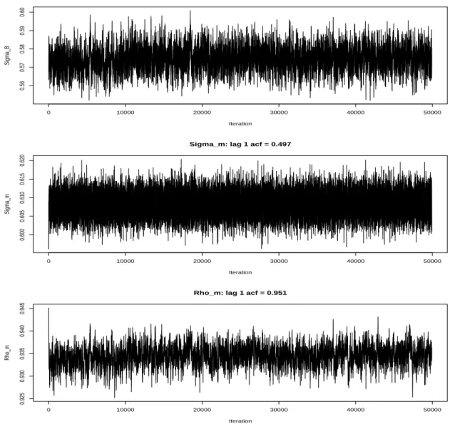
burn-in period of 10,000 Gibbs sample was used to achieve convergence, and the number

of samples used was 50,000. The convergence of the Gibbs sampler was diagnosed with

parallel chains by using the Gelman and RubinpRˆ statistic (Gelman and Rubin, 1992).

Convergence diagnostics were computed with the R coda package (Plummer et al., 2005).

See the Figure 3 for trace plots.

There was some autocorrelation in the parameters that slowed convergence, but the

effect on parameter estimation was small as the mean of the posterior estimates were

within 1% of their final estimates very early in the chain (i.e. after a few hundred

iterations). The measurement error model then yielded estimates for these parameters

as follows: σB = 0.5752(0.0062);σm = 0.6082(0.0029); ρm = 0.9347(0.0021).

These parameters suggest a large amount of variation due to assay noise. The

coef-ficient of variation due to the multiplicative technical error is ˆσm, and the correlation of the red and green components of this multiplicative effect is ˆρm which suggests that the log-ratio has significant error. These parameters will now be considered fixed in the gene

by gene survival analysis stage.

2.5.2 Data Preprocessing

Before survival models are fitted, there is some data preprocessing including gene filtering

and imputation of missing data. The large number of genes relative to the number of

(50)

0 10000 20000 30000 40000 50000

0.56

0.57

0.58

0.59

0.60

Iteration

Sigma_B

Sigma_B: lag 1 acf = 0.829

0 10000 20000 30000 40000 50000

0.600

0.605

0.610

0.615

0.620

Iteration

Sigma_m

Sigma_m: lag 1 acf = 0.497

0 10000 20000 30000 40000 50000

0.925

0.930

0.935

0.940

0.945

Iteration

Rho_m

Rho_m: lag 1 acf = 0.951

Bayesian model-based methods for the analysis of DNA microarrays with survival, genetic, and sequence data