INTEGRATED ANALYSIS OF MULTIPLE DATA SETS WITH BIOMEDICAL APPLICATIONS
Gen Li
A dissertation submitted to the faculty at the University of North Carolina at Chapel Hill in partial fulfillment of the requirements for the degree of Doctor of Philosophy in the
Department of Statistics and Operations Research.
Chapel Hill 2015
c ○ 2015
Gen Li
ABSTRACT
GEN LI: INTEGRATED ANALYSIS OF MULTIPLE DATA SETS WITH BIOMEDICAL APPLICATIONS
(Under the direction of Andrew B. Nobel and Haipeng Shen)
ACKNOWLEDGMENTS
I am very lucky to have Andrew and Haipeng as my advisors during my PhD study in the Department of Statistics and Operations Research at UNC Chapel Hill. I am greatly indebted to them for their patience, dedication, and constructive supervision. Their extraordinary empathy and valuable advice have guided me through many difficult situations and helped me make important decisions. I am also grateful for numerous enlightening and fruitful discussions with Drs. Jianhua Huang, J.S. Marron and Fred Wright. They are definitely role models in my life.
I would also like to thank my colleagues, Patrick Kimes, James Wilson, Xuan Wang, Dan Shen, Eric Lock and many others, for their insightful comments, stimulating discussions, and helpful criticism of my research. In particular, I will miss the time when Patrick and I tackled math problems together using the white board in our office.
I would not have made it without the great company of my friends. I hereby would like to thank: Juana, my beloved girlfriend, for her tremendous support and company; Minghui Liu and Dong Wang for being wonderful roommates; Dongqing Yu and Siying Li for being great neighbors; Yu Zhang and Haojin Zhai for being gym buddies; many others for sharing happiness and sorrow.
TABLE OF CONTENTS
LIST OF TABLES . . . viii
LIST OF FIGURES . . . ix
1 INTRODUCTION . . . 1
1.1 Dimension Reduction of Single Dataset . . . 2
1.2 Dimension Reduction with Multiple Datasets . . . 5
1.3 Expression Quantitative Trait Loci Analysis . . . 11
1.4 Empirical Bayes . . . 12
1.5 New Contributions and Outline . . . 14
2 SUPERVISED SINGULAR VALUE DECOMPOSITION. . . 16
2.1 Introduction . . . 16
2.2 The SupSVD Model . . . 19
2.2.1 An Equivalent Form of The Model . . . 19
2.2.2 Connections with Existing Models . . . 21
2.3 Model Estimation . . . 23
2.4 Asymptotic Analysis . . . 28
2.5 Numerical Examples . . . 29
2.5.1 Simulation Studies . . . 30
2.5.2 Breast Cancer Data . . . 33
2.6 Discussion . . . 35
2.7 Appendix . . . 36
2.7.1 Proof of Proposition 2.2.1 . . . 36
2.7.2 Proof of Proposition 2.3.1 . . . 37
2.7.4 Proof of Theorem 2.4.1 . . . 41
2.7.5 Proof of Corollary 2.4.1 . . . 43
2.7.6 Two Motivating Examples . . . 46
2.7.7 Breast Cancer Data . . . 47
2.7.8 Call Center Data . . . 48
3 SUPERVISED REGULARIZED PRINCIPAL COMPONENT ANALYSIS 53 3.1 Introduction . . . 53
3.2 Model and Likelihood . . . 55
3.2.1 Functional PCA Model . . . 55
3.2.2 SupSFPC Model . . . 57
3.2.3 Penalized Likelihood . . . 59
3.3 Computational Algorithm . . . 62
3.3.1 EM Algorithm . . . 62
3.3.2 Derivation of the EM Algorithm . . . 64
3.3.3 Tuning Parameter Selection . . . 67
3.4 Simulations . . . 68
3.5 Real Data Example: Yeast Cell Cycle Data . . . 71
3.6 Appendix . . . 75
3.6.1 Tuning Parameter Selection . . . 75
3.6.2 Government Bond Yield Data . . . 80
3.6.3 Emergency Room Visit Data . . . 82
4 MULTIPLE TISSUE EQTL ANALYSIS. . . 85
4.1 Introduction . . . 85
4.1.1 Related Work . . . 86
4.1.2 Outline . . . 88
4.2 The MT-eQTL Model . . . 88
4.2.1 Format of Multi-Tissue eQTL Data . . . 88
4.2.3 Hierarchical Model . . . 92
4.2.4 Mixture Model . . . 93
4.2.5 Marginal Consistency . . . 94
4.3 Model Fitting and Parameter Estimation . . . 95
4.3.1 Matrix eQTL . . . 95
4.3.2 Modified EM Algorithm . . . 95
4.4 Multi-Tissue eQTL Inference . . . 98
4.4.1 Detection of eQTLs Using the Local False Discovery Rate . . . 99
4.4.2 Analysis for Subsets of Tissues . . . 103
4.4.3 Assessments of Tissue Specificity . . . 103
4.4.4 Testing a Family Configurations . . . 104
4.5 Simulation Study . . . 105
4.5.1 Simulation Setting . . . 105
4.5.2 Model Fit . . . 106
4.5.3 Results . . . 106
4.6 GTEx Data Analysis . . . 108
4.6.1 Data Preprocessing . . . 108
4.6.2 Model Fit . . . 109
4.6.3 Results . . . 111
4.7 Discussion and Future Work . . . 113
4.8 Appendix . . . 116
4.8.1 Proof of Lemma 4.2.1 . . . 116
4.8.2 Proof of Theorem 4.4.1 . . . 117
4.8.3 GTEx Estimations . . . 123
LIST OF TABLES
2.1 Comparison of Parameter Estimation Accuracy . . . 32
2.2 Call Center Arrival Rates Forecasting Accuracy . . . 52
3.1 Comparison of Parameter Estimation Accuracy . . . 72
4.1 Sample Size, Sample Overlap, and Degree of Freedom . . . 105
4.2 eQTL Discoveries in a 4-Tissue Simulation . . . 107
LIST OF FIGURES
2.1 Comparison of Estimation over a Spectrum . . . 33
2.2 Breast Cancer Data - SupSVD Scores . . . 34
2.3 Breast Cancer Data - SupSVD Heat Map . . . 35
2.4 Simulation Example 1 . . . 47
2.5 Simulation Example 2 . . . 48
2.6 Breast Cancer Data - SVD Scores . . . 49
2.7 Breast Cancer Data - SVD Heat Map . . . 49
2.8 Breast Cancer Data - RRR Scores . . . 50
2.9 Breast Cancer Data - RRR Heat Map . . . 50
2.10 Call Center Data - Raw Data . . . 51
2.11 Call Center Data - Comparison of Loadings . . . 52
3.1 Simulated Smooth and Sparse Loading Vectors . . . 69
3.2 Yeast Cell Cycle Data - Raw Data . . . 73
3.3 Yeast Cell Cycle Data - Comparison of Loadings . . . 74
3.4 Clustering of Yeast Cell Cycle Data . . . 75
3.5 Yeast Cell Cycle Data - TF Activities . . . 76
3.6 Yield Data- Raw Data . . . 80
3.7 Yield Data - Comparison of Loadings . . . 81
3.8 Hospital Data - Raw Data . . . 82
3.9 Hospital Data - Comparison of Loadings . . . 83
3.10 The Day-of-Week Structure Identified by SupSFPC. . . 84
4.1 Typical Data Format, and MT-eQTL Model Input and Output . . . 89
4.2 Comparison of the Number of Significant Discoveries . . . 108
4.3 Sample Information of the GTEx Data . . . 109
4.4 Prior and Posterior Integrated Probability Mass . . . 111
4.5 Goodness of Fit for Marginal MT-eQTL Models . . . 112
4.6 Scatter Plots for a Pair of Tissues . . . 113
CHAPTER 1: INTRODUCTION
Collection of multiple data sets on the same set of samples becomes increasingly common. Many scientific research fields, such as genetics, finance and economics, now involve the analysis of multiple data types. Multiple data sets provide vast opportunities and challenges to statistics.
As an example, The Cancer Genome Atlas Network (2012) (TCGA) aims at understanding how genetic variations interact to drive cancers. The TCGA consortium collected multiple data types such as gene expression data, genotype data, and DNA methylation data from over 500 subjects for each cancer selected for study. Conceptually, different data types are inherently related and may shed light on the mechanism of disease from different perspectives. Jointly analyzing the multiple genetic data types may help us get a more comprehensive un-derstanding. Another example is the Genotype-Tissue Expression (GTEx) project (Lonsdale et al., 2013; The GTEx Consortium, 2015). The primary goal is to create a comprehensive public atlas of gene expression and regulation across multiple human tissues. Noticing the commonality among tissues, one may borrow strength across tissues when studying genetic regulation in one tissue. Moreover, the joint analysis of multiple tissues may expand the scope of single tissue analyses by addressing more fundamental biological questions about the nature and source of variation among tissues.
In this dissertation, we develop two statistical methodologies for integrated analysis of multiple data sets: one issupervised dimension reduction and the other is multi-tissue eQTL model. For the first topic, we are interested in dimension reduction of a primary data set, with the presence of an auxiliary data set. The goal is to exploit the auxiliary information to improve the accuracy and interpretability of the reduced primary data. Motivated by many applications, we assume the auxiliary data set potentially drives the underlying structure of the primary data. We develop a latent variable model to account for the supervision effect in dimension reduction. For the second topic, we are interested in studying eQTL, or significant gene-SNP associations, in multiple tissues. The goal is to utilize genetic data across multiple tissues to increase eQTL detection power and improve tissue-specificity assessment. We develop a hierarchical Bayesian model to jointly analyze gene-SNP associations in multiple tissues.
In this chapter, we briefly review some relevant concepts and existing methods. In Sec-tion 1.1, we introduce several dimension reducSec-tion methods for a single multivariate data set, including Singular Value Decomposition (SVD), Principal Component Analysis (PCA), and factor analysis. In Section 1.2, we extend to methods involving multiple data sets, such as Sufficient Dimension Reduction (SDR), Canonical Correlation Analysis (CCA), and par-simonious multivariate regression. In Section 1.3, we give an overview of the expression quantitative trait loci (eQTL) analysis. In Section 1.4, we briefly introduce the empirical Bayes framework. A summary of our contributions and the outline of the dissertation is given in Section 1.5.
Notation: Throughout the dissertation, without special notification, we use bold capital
letters (e.g., X, Y) to denote matrices, bold small letters (e.g., u, v) to denote column vectors, and plain letters (e.g.,λ,c) to denote scalars. For a random data matrix, we assume
each row corresponds to a sample and each column corresponds to a variable.
1.1 Dimension Reduction of Single Dataset
SVD is a popular matrix decomposition approach. It factorizes a matrix into a sum of several unit-rank layers. Formally, let X be an n×p data matrix of rank k, where k ≤
min(n, p). The SVD ofX can be written as
X=UDVT =
k
X
i=1
diuiviT
where U = (u1,· · ·,uk) is an n× k matrix of orthonormal left singular vectors, V =
(v1,· · · ,vk) is ap×kmatrix of orthonormal right singular vectors, andD= diag(d1,· · ·, dk)
is a diagonal matrix with positive singular values d1 ≥ · · · ≥dk>0. In particular, diuivTi is
theith unit-rank layer with Frobenius normdi. If all singular values are distinct, the
decom-position is uniquely defined. When some of the di’s are equal, the column space spanned by
the corresponding left (or right) singular vectors is unique, while the specific singular vectors are determined up to an orthogonal rotation.
SVD can be used as a dimension reduction approach. We can obtain a low rank approxi-mation ofX by taking the summation of the first few unit-rank layers. In particular, for any rank r≤k, we have
r
X
i=1
diuiviT = arg min
C∈Rnr×p
kX−CkF = arg min C∈Rnr×p
tr{(X−C)(X−C)T}
where Rnr×p is the set of all n×p matrices with rank r, and k · kF represents the Frobenius
norm. In the sense, SVD provides the best low rank approximation of a matrix in terms of minimizing the Frobenius norm of the difference between the low rank matrix and the original one.
Principal Component Analysis
criterion:
arg max {v1∈Rp:kv1k2=1}
var(v1Tx),
and subsequent loading vectors (k= 2,· · ·, p) are obtained by solving
arg max
{vk∈Rp:kvkk2=1,vTkvj=0,j=1,···,k−1}
var(vkTx).
It is easy to see that the PC loadings are the eigenvectors ofΣon population level.
When the true Σ is unknown, PC loadings can be estimated from a sample covariance matrix. This is closely related to the SVD method. Let X denote an n×p data matrix where each row is an independent identically distributed (i.i.d.) sample with mean µ and covarianceΣ. Without loss of generality, we assumeXhas been column centered. PCA can be computed by the SVD of X. In particular, if we write the SVD ofX asUDVT where U is the left singular matrixV is the right singular matrix andDis the diagonal singular value matrix, the columns ofUDcorrespond to PC scores and the columns ofVcorrespond to PC loadings. Alternatively, one may also obtain PC loadings by decomposingXTX, and obtain PC scores by decomposingXXT.
Recently, many variants of PCA have been investigated and adapted for different applica-tions. For example, Shen and Huang (2008b) proposed a sparse PCA method by imposing`1
regularized PCA methods. Factor Analysis
Factor analysis describes variability of correlated variables in terms of a small number of latent factors. Formally, the factor model for a length-prandom vector xis
x=µ+Lf +ε
whereµis a mean vector,f is an length-r random vector (r < p) with entries being uncorre-lated latent factors,L is a p×r loading matrix, and εis a p×1 error vector. We assume f has mean zero and covarianceI, and is independent ofεwhich has mean zero and covariance Σ. Hence the covariance of x is LLT +Σ. One may impose different covariance structures
onΣ to form different factor models.
To estimateµ,L, andΣin a factor model, people usually use theExpectation-Maximization
(EM) algorithm. It is an iterative algorithm alternating between an E step and an M step. In the E step, we calculate the conditional distribution of the latent factorf given the observed dataxand parameters estimated from the previous iteration; in the M step, we maximize the conditional expectation of the joint likelihood of xand f with respect to model parameters.
Factor analysis is closely related to PCA, but they are not the same. By definition, the PC loadings ofx are the eigenvectors ofLLT +Σ, which are not necessarily the columns of L. However, when Σis isotropic (i.e., Σ=σ2I) and L has orthogonal columns, it is easy to
see the firstr eigenvectors of LLT +Σ are proportional to the columns ofL. In fact, when Σ=σ2I, the factor model is the probabilistic PCA model proposed by Tipping and Bishop (1999).
1.2 Dimension Reduction with Multiple Datasets
Sufficient Dimension Reduction
Assume we have a univariate responsey and a multivariate predictor vectorx∈Rp. The
ofx, denoted by R(x), that lies in a lower dimensional subspace Rr (r < p) and contains all relevant information about y in x. Formally, a reduction R(·) : Rp 7→ Rr is sufficient if it satisfies one the following conditions:
(1) x|(y, R(x))∼x|R(x), (2) y|x∼y|R(x),
(3) x |=y|R(x),
where ∼ means identically distributed and |= means independent. These conditions are equivalent when (y,x) has a joint distribution. Different conditions may be useful in different situations. For example, when the response is assumed fixed, only condition (1) makes sense since it does not require y to be random; for fixed design where x is assumed fixed, only condition (2) is meaningful.
The sufficient reductionR(·) can be of any form. In the extreme case where no reduction is available, R(·) is a one-to-one mapping of x. For simplicity, people usually assume that
R(·) is a collection of linear transformations: R(x) = (βT1x,· · ·,βTrx)T =BTx, where B =
(β1,· · ·,βr) is ap×rcoefficient matrix. The column space ofBis called adimension reduction subspace, denoted by SB. Since any superspace of SB also contains all relevant information about y inx, the dimension reduction subspace is not unique. Under mild conditions, Cook (1996) shows that the intersection of two dimension reduction subspaces is still a dimension reduction subspace. Consequently, the inferential target in sufficient dimension reduction is often taken to be the intersection of all dimension reduction subspaces which is uniquely defined. It is called thecentral subspace, denoted by Sy|x.
There has been a lot of efforts devoted to the estimation of central subspace. In particular, there are two major lines: moment-based methods and likelihood-based methods. Li (1991) proposed a sliced inverse regression (SIR) approach that exploits the first moment ofxgiven
SIR and SAVE and move beyond (see Cook and Ni, 2005; Ye and Weiss, 2003; Yin and Cook, 2003, for example). Cook and Forzani (2009) proposed a maximum likelihood estimator of the central subspace based on Gaussian assumptions. They demonstrated the method outperforms moment-based methods and is robust against deviations from normality.
Parsimonious Multivariate Regression
In multivariate regression problems, the response has multiple variables. In particular, assumingy = (y1,· · ·, yq)T ∈Rq and x = (x1,· · ·, xp)T ∈Rp, a multivariate regression has the following form
y=µ+BTx+ε
whereµis aq×1 intercept vector,Bis ap×qcoefficient matrix, andεis an error vector with mean zero and covariance Σ. Without loss of generality, in the context we always assume that all variables are centered beforehand so we get rid of the intercept term. When multiple observations are available, the model can be written in the matrix form as
Y =XB+E
where Y is an n×q response matrix, X is an n×p design matrix, and each row of E is i.i.d. with mean zero and covarianceΣ. In particular, we assume columns of X are linearly independent to avoid indeterminacy.
Ordinary least square (OLS) is one of the most popular approaches to estimate the re-gression coefficient matrixB. It minimizes the following criterion
b
BOLS= arg min B
kY−XBk2
F= arg min
B
tr{(Y−XB)T(Y−XB)}
wherek · kF is the Frobenius norm. The above problem has a unique closed-form solution as
b
whenXhas full column rank. OLS is equivalent to maximum likelihood estimate (MLE) when the random noise has a multivariate Gaussian distribution. Under Gaussian assumption, the log likelihood of the observed data is proportional to−tr{(Y−XB)Σ−1(Y−XB)T}. When Σ is isotropic, i.e., Σ = σ2I, the MLE has the same object function as OLS; when Σ is any positive definite matrix, using elementary matrix calculus calculations we can derive the closed form solution of MLE to be the same as that of OLS as well. Namely, BbMLE ≡BbOLS under normality.
In high dimension, overfitting issue may arise in estimation. Two primary solutions have been extensively studied: one is feature selection, and the other is feature extraction. The idea of feature selection is to use a subset instead of all of the p variables to construct the model. The idea of feature extraction is to transform the data from thep-dimensional space to a low-dimensional subspace. Both are achieved by adding structural constraints on the coefficient matrixB. In particular, feature selection can be achieved by imposing sparsity on B. Unimportant variables are removed from the analysis by the device of zero coefficients in B. Various sparse multivariate linear regression methods have been studied in literature (cf. Turlach et al. (2005), Yuan et al. (2007), Lee and Liu (2012), Rothman et al. (2010)).
To realize feature extraction, one general approach is to impose a rank constraint on the co-efficient matrix. Consider the multivariate regression model with the constraint rank(B) =r
wherer is a prespecified number much smaller than min(p, q, n). We write the QR decompo-sition ofBasQRT whereQis aq×r matrix,Ris ap×rmatrix. As a result, the constrained regression model can be written as
Y=XQRT +E.
OLS criterion is commonly used to estimateB in RRR
b
BRRR = arg min rank(B)=r
kY−XBk2
F.
Again, this is equivalent to MLE when the random error is Gaussian with isotropic covariance structure. The explicit solution is given in Reinsel and Velu (1998) as
b
BRRR= (XTX)−1XTYHHT
where H = (h1,· · ·,hr) and hi is the ith eigenvector of YTX(XTX)−1XTY. When the
random error is Gaussian but with arbitrary positive definite covariance structure, the OLS is not equivalent to the MLE anymore. The closed form MLE solution is given in Izenman (1975). Recently, Chen et al. (2012) and Chen and Huang (2012) combined feature selection and feature extraction by imposing sparsity on the low rank coefficient matrix estimation. Numerical studies show the proposed sparse RRR methods have more appealing performances in many situations.
Envelope model (Cook et al., 2010) is another parsimonious variation of multivariate regression. The motivation comes from the observation that some variations in response might be unrelated with the predictor. In that case, by separating the material variation from the immaterial one and only focusing on the former, one expects to reduce the coefficient estimation variability. In particular, the coordinate version of the envelope model is
Y = XΛΓT +E Σ = ΓΩΓT +Γ0Ω0ΓT0
whereΛΓT is the low rank coefficient matrix, (Γ,Γ0) is a q×q orthogonal matrix, Σis the
covariance structure for each i.i.d. row of E, and Ω and Ω0 are two positive definite
matri-ces. YΓ envelops the material variation in the response, and YΓ0 envelops the immaterial
have been studied in Su and Cook (2011), Su and Cook (2012), Su and Cook (2013), Cook and Su (2013) and Cook et al. (2013).
Canonical Correlation Analysis
Unlike regression models, CCA focuses on examining correlation structures between two multivariate random vectors. It treats both random vectors equally, without assuming one to be response and the other to be predictor. The idea of CCA is to find linear combinations such that the correlations between the two are sequentially maximized. Assume we have multivariate vectors x = (x1,· · · , xp)T ∈ Rp and y = (y1,· · · , yq)T ∈ Rq. The first pair of canonical loadings (u1,v1) is the solution of the following optimization problem
max u∈Rp,v∈Rq
corr(uTx,vTy).
For identifiability purpose, we need to require both loading vectors have norm 1. The sub-sequent pairs of loadings are defined in a similar way under the orthogonal constraint that uTi uj =vTi vj =δij whereδij is the kronecker delta.
Let Σx and Σy denote the covariance matrices of x and y respectively, and let Σxy = cov(x,y) andΣyx = cov(y,x). With some algebraic calculations, we know the loading vectors ui’s are the eigenvectors ofΣ−x1ΣxyΣ−y1Σyxandvi’s are the eigenvectors ofΣ−y1ΣyxΣ−x1Σxy. Correspondingly,uTi xandvTi yare called the ith canonical scores. When the true covariance matrices are unknown, we can replace them with sample covariance matrices. LetXandYbe data matrices withni.i.d. samples. We haveΣcx= 1nXTX,Σcy= n1YTY,Σdxy = 1nXTY and
d
Σyx = n1YTX. The canonical loadings are estimated accordingly through eigendecomposition of the product of sample covariance matrices.
results.
1.3 Expression Quantitative Trait Loci Analysis
Genetic variation in a population is commonly studied through the analysis of SNPs, which are variants occurring at specific sites in the genome. Differences among these vari-ants drive primary phenotypic differences between members of the population. For humans these differences range from physical characteristics to disease susceptibility. Mediating the connection between genetic variation and resulting phenotypes are the effects of SNPs on the expression of different genes. The analysis of eQTL seeks to identify genetic variants that affect the expression of one or more genes: a gene-SNP pair for which the expression of the gene is associated with the value of the SNP is referred to as an eQTL. Enabled by high-throughput sequencing, eQTL analysis has proven to be an effective approach for the discovery of genomic variants that influence expression, and a potentially useful tool in the study of pathways and networks that underlie disease in human and other populations. For an overview of eQTL analysis and disease mapping, see Cookson et al. (2009), Mackay et al. (2009), Rockman and Kruglyak (2006), and the references therein. Kendziorski and Wang (2006) and Wright et al. (2012) survey existing statistical and computational methods for eQTL analysis, respectively.
To date, most eQTL studies have considered the effects of genetic variation on expression within a single tissue. Nonetheless, these studies have provided enhanced understanding of gene regulation and the etiology of various diseases, cf. Franke and Jansen (2009) and Westra et al. (2013). A natural next step in understanding genomic variation of expression is the simultaneous analysis of eQTLs in multiple tissues. Multi-tissue eQTL analysis has the potential to improve the findings of single tissue analyses by borrowing strength across tissues, and to expand the scope of single tissue analyses by addressing more fundamental biological questions about the nature and source of variation between tissues.
studies is that a SNP may be associated with the expression of a gene in some tissues, but not in others. Thus a full multi-tissue analysis must identify complex patterns of association across multiple tissues. We will refer to an eQTL as ’common’ if association is present in all available tissues, and ’tissue-specific’ if association is present in at least one tissue, but not all. Until recently, understanding of multi-tissue eQTL relationships was limited by a shortage of true multi-tissue data sets, requiring the assimilation of data or results from different stud-ies (one for each tissue) involving distinct populations, measurement platforms, and analysis protocols,cf.Emilsson et al. (2008) and Xia et al. (2012).
Recently, a number of human true multi-tissue eQTL data sets have been collected, for example by Dimas et al. (2009) and Nica et al. (2011), although these contain relatively few tissues. By contrast, the GTEx initiative (Lonsdale et al. (2013)) and related projects are generating eQTL data from dozens of tissues in several hundred individuals, greatly expanding our potential understanding of the variation and specificity of eQTL effects across multiple tissues. The size and complexity of these emerging multi-tissue data sets has created the need to expand existing statistical tools for eQTL analysis.
1.4 Empirical Bayes
Empirical Bayes methods are statistical inference procedures that combine Bayesian mod-els with Frequentist estimation procedures. In Bayesian hierarchical modmod-els, parameters of interest are treated as random variables with prior distributions in which the parameters are called the hyperparameters. A typical Bayes approach would either integrate out the hyper-parameters or set them to be values based on some subjective prior knowledge. For empirical Bayes methods, the hyperparameters are estimated from observed data through marginal maximum likelihood which is a typical Frequentist approach. Conceptually, empirical Bayes approaches fully utilize the information in the observed data.
such that the observations are normally distributed as
x∼ N(θ, σ2I).
We are interested in estimating the parameter vectorθusing the single observation vector x. For simplicity, we assume σ2 is known. In Frequentist inference, the least square estimate of
θ is just x.
In Bayesian framework, the parameter vector θ is assumed random, and one can impose a flexible prior distribution on θ based on prior knowledge. In particular, we set the prior distribution of θ to be N(0, τ2I) where τ2 is an unknown hyperparameter. The posterior distribution of θ given xis
θ|x∼ N
τ2 τ2+σ2x,
τ2σ2 τ2+σ2
.
Consequently, for any fixed τ2, the Bayes estimate of θ is [τ2/(τ2+σ2)]x. Notice the Bayes
estimate depends on the subjective choice of the hyperparameter τ2.
The empirical Bayes approach takes advantage of the flexible Bayesian model while esti-mating the hyperparameter from the data. In particular, from the marginal distribution ofx we know
E
1−(p−2)σ
2
kxk2 2
= τ
2
τ2+σ2
for any p > 2. We can substitute this into the Bayes estimate and get the empirical Bayes estimate as
1− (pk−2)σ2
xk2 2
x. This estimate has the same form with the James-Stein estimate (Stein, 1956). It has been proved (Efron and Morris, 1973) that the empirical Bayes estimate strictly outperforms the Frequentist estimate whenp ≥3 in terms of the mean square error for any true value.
of differential expression and co-expression in gene microarrays, cf. Kendziorski et al. (2003), Newton et al. (2004), Smyth (2004), Efron (2008), and Dawson and Kendziorski (2012).
1.5 New Contributions and Outline
In this dissertation, we focus on two topics of the integrated analysis of multiple data sets, i.e., supervised dimension reduction and multi-tissue eQTL analysis. We shall illustrate that in both studies integrated analysis outperforms separate analysis by borrowing strength across data sets. Briefly, the remainder of the dissertation is organized as follows:
to identify auxiliary variables with no supervision effect. The resulting methodology subsumes the original supervised PCA method, as well as existing regularized PCA methods, such as functional PCA and sparse PCA as special cases. Numerical studies show the proposed method outperforms competitive approaches in terms of low-rank structure recovery accuracy in a wide range of settings. In an application example concerning yeast cell cycle-related genes, the supervised regularized PCA method takes advantage of auxiliary transcription factors binding information and captures underlying cyclic patterns of gene expressions in two cell cycles. Moreover, it simultaneously identifies important transcription factors that regulate cell cycles, which is not achieved by other dimension reduction methods.
CHAPTER 2: SUPERVISED SINGULAR VALUE DECOMPOSITION AND ITS ASYMPTOTIC PROPERTIES
2.1 Introduction
As high dimensional data become increasingly common, dimension reduction becomes more and more important, since it is easier to visualize and analyze a low dimensional struc-ture in high dimensional data. SVD is a fundamental tool used in multivariate analysis to decompose a high-dimensional data matrix into a sum of unit-rank layers ordered by impor-tance. The first few layers, which often capture the majority of the variation, act as a low rank approximation or dimension reduction of the original data.
However, one drawback of SVD is that it only makes use of a single data set, and by default the resulting dimension reduction cannot incorporate any additional information that may be relevant. When multiple related data sets are available on the same set of samples, sharing information across data sets may lead to recovery of a low rank structure that is more interpretable. Several approaches have been developed for analyzing multiple data sets. For example, Lock et al. (2013) develops an integrative approach to study joint and individ-ual variations simultaneously; Bair et al. (2006) develops a supervised principal component regression method to select predictors and do prediction. In this chapter, we propose a su-pervised SVD (SupSVD) model to achieve dimension reduction that incorporates auxiliary information. We assume that the auxiliary data set, which we refer to as the supervision, is a potential driving factor for the low rank structure of theprimarydata of interest.
potentially get a better understanding of if we take advantage of the supervision (SNP) data. We now introduce the SupSVD model using matrix notation. Let X denote the data matrix of primary interest which has nrows (or samples) and p columns (or variables). Let Y denote the supervision data matrix which has n rows (matched with X) and q columns. We assume that the intrinsic information inXis low dimensional with rankr(r ≤min(n, p)), and is possibly driven byY, in a linear fashion. In matrix form, the SupSVD model can be expressed as follows:
X=UVT +E,
U=YB+F,
(2.1)
where U is an n×r latent score matrix, V is a p×r full-rank loading matrix, and B is a
q×r coefficient matrix, withF andE beingn×r and n×p error matrices, respectively. Overall, the SupSVD model captures situations in which X has an intrinsic low rank structure and the structure is partially affected byY. The first equation in (2.1) is motivated by the additive-multiplicative low-rank approximation model for SVD, as in Dozier and Sil-verstein (2007) and Shabalin and Nobel (2013). It indicates that the observed data matrixX consists of the low rank structureUVT plus measurement errors E. We use a multivariate linear regression model to capture the potential supervising effect of Y on the score matrix U. In particular, the matrixFcaptures information inUthat cannot be explained byY. We note that very recently Fan et al. (2014) proposed a projected PCA method that generalizes the second equation of (2.1) to a semi-parametric model.
error term, consisting of a few latent factors and noise. The name of the model comes from the fact that the latent factors are modeled with surrogate variables. Both models are related to but different from the SupSVD model we propose here.
Compared with the SVD, the SupSVD model incorporates the auxiliary information in Y. The potential advantages of SupSVD over SVD are two-fold. First, using additional infor-mation may help reveal interesting patterns that might otherwise be undiscovered. Second, the low rank structure recovered by the SupSVD model might have superior interpretability. Evidence can be found in the simulated examples in the appendix, Section 2.7.6. Overall we find that SupSVD performs favorably when the supervision information is indeed a driving factor of low rank data. When auxiliary data are irrelevant, for example in Case 2 of Section 2.5.1.1, SupSVD automatically adapts to the situation and performs as well as SVD.
There is a rich literature on dimension reduction of a data matrix X in the presence of auxiliary information Y, for example sufficient dimension reduction Cook and Ni (2005), supervised principal components Bair et al. (2006), and principal fitted components Cook (2007); Cook and Forzani (2008). Moreover, reduced rank regression (RRR) Izenman (1975); Reinsel and Velu (1998) can also be viewed as a dimension reduction approach for X if we regressXonY. The focus of most existing methods is to find a dimension reduced version of Xthat keeps all the information aboutY. This is different from the scope of the current paper. Here our primary goal is to identify low rank structure ofX, whether or not the structure is related to the auxiliary informationY. The auxiliary informationY offers guidance for the dimension reduction ofX. To the best of our knowledge, our work is the first to address this topic.
the appendix, Section 2.7.
2.2 The SupSVD Model
In this section, we describe the SupSVD method in detail. Section 2.2.1 gives an equivalent formulation of the model, and discusses identifiability conditions. Section 2.2.2 establishes connections of the proposed model with some existing methods.
2.2.1 An Equivalent Form of The Model
In Model (2.1), if we substitute the latent matrix U in the first equation with the second equation, we get an equivalent form for the SupSVD model as:
X=YBVT +FVT +E. (2.2)
Without loss of generality, we assume that both X and Y are column-centered; hence, the model does not have intercepts. The random matrices E and F are assumed independent. Each entry of the error matrixE is independently identically distributed (i.i.d.) with mean zero and varianceσ2e. This follows the signal-plus-noise model for matrix reconstruction, cf. Shabalin and Nobel (2013), as well as ther-component spiked covariance model for PCA, cf. Johnstone (2001); Paul (2007). Each row ofFis i.i.d. with mean zero and covariance matrix Σf, which is an unknownr×r positive definite matrix.
Furthermore, Model (2.2) can be viewed as a special setup of a multivariate linear regres-sion model
X=Yβ+ε
where the coefficient matrix β is BVT of rank min(r, q), and the random noise matrix ε is FVT+E. The rows of the noise matrixεare i.i.d. with covarianceΣequal toVΣfVT+σe2Ip
whereIp is thep×pidentity matrix.
data X using Y. Namely, we want to estimate YBVT +FVT, where YBVT is the deter-ministic part andFVT is the random part. The deterministic signal is driven byY and the random signal captures important structures from unknown sources. The two parts are re-lated through the common loading matrixV, and together they form the underlying low rank representation forX. In practice, we substitute all model parameters by estimates obtained from the observed data, and replace the random matrix Fby its best unbiased prediction.
The SupSVD model (2.2) is identifiable in terms of the coefficient matrixβ =BVT and
the covariance matrix Σ=FVT +E, but unidentifiable in terms of the specific parameters B, V, Σf, and σ2e. To see this, let B? = BQ, V? = VQ, and Σ?f = QTΣfQ for any
r×r orthogonal matrixQ. It is easily seen that BVT =B?V?T and VΣfVT =V?Σ?fV?T. Namely, the two sets of parameters lead to the same Model (2.2). In particular, we define two sets of parameters to beequivalentwhen they give identical likelihood functions (see (2.6) below).
For regression purpose knowing β andΣis enough, but for dimension reduction purpose we need to obtain all specific parameters since each parameter has an important interpreta-tion. For example, the columns ofV can be interpreted as projection directions; the matrix Σf gives the covariance structure of latent scores; each column of B indicates how the su-pervision matrix Y is related with the corresponding score vector. Therefore we impose the following constraints to identify the model.
(1) Thep×r matrixV has orthonormal columns, i.e.,VTV =I r;
(2) Ther×r matrix Σf is diagonal with r distinct positive eigenvalues;
(3) The columns ofV are sorted in the descending order in terms of column norms ofXV, and the first entry of each column is positive.
out column and sign switches. In addition, we also assume that the supervision data matrix Yhas linearly independent columns; in practice, one can discard linearly dependent columns inY. Under these conditions, the SupSVD model is identifiable. Hereafter, without special notice, we assume that the model satisfies all the aforementioned identifiability conditions. We comment that the identifiability conditions help us identify the unique representative in an equivalence class.
Proposition 2.2.1. In Model (2.2), for any parameter set(B,V,Σf, σ2e)such that the largest
r eigenvalues of Σ=VΣfVT +σe2I are distinct and greater than the remaining eigenvalues,
there exists an unique parameter set that is equivalent with (B,V,Σf, σe2) and satisfies the
identifiability conditions.
For cases in which two or more of the first r eigenvalues of Σ are equal, the above con-ditions are not sufficient for identifiability, and one may have to impose constraints onB as well. However, in real data examples, equal-eigenvalue cases rarely occur. Therefore, we can reasonably restrict our scope to models that satisfy the identifiability conditions.
2.2.2 Connections with Existing Models
The SupSVD model (2.2) has close connections with several existing models. On the one hand, when B = 0, i.e., when the score matrix U equals to the random matrix F, Model (2.2) reduces to
X=FVT +E. (2.3)
In Model (2.3), each row ofX is i.i.d. with mean zero and covariance matrixVΣfVT +σ2eIp,
which is exactly the r-component spiked covariance model for PCA, cf. Johnstone (2001); Paul (2007); Shen et al. (2013). In the model, the r columns of V are the first r principal component (PC) loadings, and the columns ofXV are the corresponding PCs. Note that the PCA model is unsupervised, as the matrix Y does not appear in the model.
SupSVD model reduces to
X=YBVT +E, (2.4)
where for identifiability purposes we letBhave orthogonal columns. We note that Model (2.4) is the reduced rank regression (RRR) model (Izenman, 1975; Reinsel and Velu, 1998) with isotropic covariance structure (we will refer to isotropic RRR as RRR). The matrixC=BVT is the rankr coefficient matrix whose least square estimator is explicitly given in Reinsel and Velu (1998). In this case, the true underlying structure ofXisYBVT, whose column space is a subspace of the column space ofY. In other words, the underlying structure is fully driven by the supervision information. We therefore refer to the RRR model as fully supervised.
The SupSVD model (2.2) is also connected with the envelope model that was recently proposed by Cook et al. Cook et al. (2010) and further developed in (Cook et al., 2013; Cook and Su, 2013; Cook and Zhang, 2015; Su and Cook, 2011). The envelope model is a parsimonious model for multivariate regression that is based on the assumption that variation in the response can be divided into two parts: a material part that is related to the predictor, and an immaterial part that is unrelated to the predictor. The envelope model achieves substantial efficiency gain in parameter estimation by focusing on the material part of the response. The coordinate version of the envelope model can be written as
y = α+Γηx+ε (2.5)
Σ = ΓΩΓT +Γ0Ω0ΓT0.
Hereyis ap-dimensional response, xis aq-dimensional predictor,Γ isp×rsemi-orthogonal matrix andη is anr×q matrix. The product ofΓ andη acts as a coefficient, whileα and ε
are the intercept and the random error. The random errorεhas covariance matrixΣdefined in the second equation, in which (Γ,Γ0) is orthogonal, and Ωand Ω0 are positive definite.
covariance of (2.2) is slightly more specific than that of (2.5). However, we note that the two models arise in the analysis of different problems, and that they have different applications and interpretations. The SupSVD model attempts to extract a low rank representation of a primary data matrix, and is intended for dimension reduction problems in which auxiliary data is present. The goal of the envelope model is to reduce the variation of coefficient estimation in regression problems. Here we impose identifiability conditions on the model and estimate each parameter, as the parameters are directly interpretable in the context of dimension reduction. In Cook et al. (2010) the authors focus on identifying estimable subspaces that are spanned by the parameters of their model; the parameters themselves are of less importance. In addition, fitting of the SupSVD and envelope models is carried out in fundamentally different ways. We describe a computationally efficient EM type algorithm to fit the model (2.1) for which the likelihood of the observed data usually converges to a local maximum after a few iterations. In order to fit the envelope model, the authors of Cook et al. (2010) directly maximize the likelihood function, which involves optimization over a Grassmann manifold. We compared the computational speeds of both methods using various simulations, and in general the EM algorithm is faster.
SupSVD can be viewed as a general model for supervised dimension reduction. It encom-passes unsupervised PCA and fully supervised RRR as two extremes. When the auxiliary information is irrelevant to low rank structure of the primary data, the SupSVD model re-duces to the PCA model; when the underlying structure is totally driven by the auxiliary data, the SupSVD model reduces to the RRR model. It also connects with the envelope model from a multivariate regression point of view.
2.3 Model Estimation
of this section.
Under the normality assumption for E and F, we can obtain the distribution of the observed dataX according to (2.2) as
vec(XT)∼ Nnp vec(VBTYT), In⊗(VΣfVT +σe2Ip)
,
where vec(·) is the column-stacking operator and ⊗is the Kronecker product. Thus the log likelihood ofX can be expressed explicitly as
L(X) =−np
2 log(2π)−
n
2log det (VΣfV
T +σ2 eIp)
−1
2tr (X−YBV
T)(VΣ
fVT +σe2Ip)−1(X−YBVT)T
,
(2.6)
where the parameters satisfy the identifiability conditions discussed above.
One way to estimate the parameters is to directly maximize the likelihood function (2.6) under the identifiability conditions. However, a direct constrained maximization is challenging for two reasons: 1)V appears in both the mean and the variance of the normal distribution; and 2) the constrained parameter space is not convex. As a remedy, we propose a modified EM algorithm, namely anexpectation-maximization-standardization (EMS)algorithm, to ef-ficiently estimate the model parameters. The additional standardization step guarantees that the parameter estimates satisfy the identifiability conditions.
The latent matrix U in Model (2.1) naturally suggests the possibility of using the EM algorithm for parameter estimation. The joint log likelihood ofX and U, i.e.,L(X,U), can be separated into two parts: the conditional log likelihood of X given U, and the marginal log likelihood ofU. In detail,
where
vec(XT)|U ∼ Nnp vec(VUT), σ2eInp
, and (2.8)
vec(UT) ∼ Nnr vec(BTYT),In⊗Σf
. (2.9)
The benefit of this separation is that the parameters (B,Σf) are isolated from (V, σ2e), and each parameter only contributes to one part of the likelihood. Using (2.7) the joint log likelihood has the following form:
L(X,U) ∝ −nplogσe2−σe−2tr (X−UVT)(X−UVT)T
−nlog detΣf −tr (U−YB)Σ−f 1(U−YB)
T
.
Below we describe the steps of the EMS algorithm, which is presented as Algorithm 1 at the end of this section. We use θ(i) = (B(i),V(i),Σ(i)
f , σe2 (i)
) to denote the parameter estimates obtained in theith iteration, which satisfy the identifiability conditions.
E Step: We calculate the conditional expectation of L(X,U) with respect to U given X and θ(i), i.e., EU(L(X,U)|X, θ(i)). The conditional distribution of U given X and the previous parameter estimationθ(i) is
vec(UT) |X ∼ N
vec
Θ(Ui)|XT
, In⊗Ω(Ui)|X
, (2.10)
where
Θ(Ui)|X = EU(U|X) =
YB(i)
σ2e(i)Σ(fi)−1
+XV(i) Ir+σ2e (i)
Σ(fi)−1 −1
,
Ω(Ui)|X =
Σ(fi)−1+σe−2(i)Ir
−1 .
Note that the conditional expectation ofUgivenXis a weighted average ofYB(i)andXV(i), where the weights are determined byσe2(i) andΣ(fi).
is not convex. As the joint distribution ofXandUis identifiable even without the side condi-tions, we propose a modified EM algorithm that bypasses the constrained optimization prob-lem. More specifically, we first obtain the unconstrained optimizers of EU(L(X,U)|X, θ(i)), and then find the unique set of parameters that is equivalent to the optimizers in terms of the SupSVD model, and that satisfies the identifiability conditions.
The unconstrained optimization problem can be solved analytically. Setting partial deriva-tives of EU(L(X,U)|X, θ(i)) with respective to each parameter to zero, we obtain
b
B = (YTY)−1YTEU(U|X, θ(i)), (2.11) b
V = XTEU(U|X, θ(i)) h
EU(UTU|X, θ(i)) i−1
, (2.12)
c Σf =
1
nEU
h
(U−YB)b T(U−YB)b |X, θ(i) i
, (2.13)
c
σ2
e =
1
npEU
h
tr((X−UVbT)(X−UVbT)T) |X, θ(i) i
, (2.14)
where the corresponding conditional expectations can be obtained from (2.10). Details can be found in the appendix, Section 2.7.3.
S Step: The unconstrained optimizers (Bb,Vb,Σcf,cσe2) in (2.11)–(2.14) typically satisfy the condition of Proposition 2.2.1. In this case, we can obtain the unique equivalent set of parameters that satisfy the identifiability conditions. In particular, we perform SVD on
b
VΣcfVbT to obtain the following eigen-decomposition:
V(i+1)Σ(fi+1)V(i+1)T =VbΣcfVbT,
where the columns ofV(i+1) are the orthonormal eigenvectors and the diagonal entries of the diagonal matrix Σ(fi+1) are the eigenvalues. In practice, the eigenvalues are almost always positive and distinct, so that the matrices V(i+1) and Σ(fi+1) satisfy the identifiability con-ditions and are unique up to a column reordering. Then, we set B(i+1) = BbVbTV(i+1) and
σ2 e
(i+1)
=cσe2. It is easy to see that
Lastly, we reorder the columns of V(i+1), and accordingly the columns of B(i+1) and the rows/columns ofΣ(fi+1), in order to ensure that the column norms ofXV(i+1)are decreasing. As a result, we get parameter estimatesθ(i+1) = (B(i+1),V(i+1),Σ(fi+1), σe2(i+1)) for the (i+ 1)th iteration.
Each step of the EMS algorithm has an analytical expression and can be computed effi-ciently. Our numerical studies indicate that the algorithm is insensitive to initial values. In practice, we use the naive estimates from SVD as the initial values. The following proposition guarantees convergence of the EMS algorithm to a local optimum.
Proposition 2.3.1. In each iteration of the EMS algorithm, the log likelihood of the observed data L(X) is monotonically nondecreasing. Therefore, the EMS algorithm always converges to some stationary point (maybe local maximum).
Algorithm 1 The EMS Algorithm for Parameter Estimation under the SupSVD Model
1: Set initial values for the parameters (B(0),V(0),Σ(0) f , σ2e
(0)
);
2: whileL(X|θ(i+1))− L(X|θ(i))>thresholddo
3: E Step: Derive the conditional distribution (2.10) givenθ(i) = (B(i),V(i),Σ(fi), σ2e(i));
4: M Step: Obtain the unconstrained optimizer (Bb,Vb,Σcf,cσe2) from (2.11)-(2.14);
5: S Step: Standardize (Bb,Vb,Σcf,cσe2) to get θ(i+1) = (B(i+1),V(i+1),Σ(i+1) f , σe2
(i+1)
) that satisfy the identifiability conditions;
6: Seti←i+ 1.
7: end while
2.4 Asymptotic Analysis
In this section, we state the consistency and asymptotic normality of the SupSVD param-eter estimates. Since the SupSVD model is overparamparam-eterized, i.e., unidentifiable without side conditions, standard asymptotics from the maximum likelihood framework do not apply directly. Instead, we refer to the asymptotic results in Shapiro (1986) for overparameterized structural models. A similar treatment can be found in Cook et al. (2010).
Specifically, we first focus on the estimable functions β=BVT and Σ=VΣfVT +σ2eI, which uniquely define the likelihood function. In order to fit our analysis into the framework of (Shapiro, 1986), we rewrite the parameters as
φ= vec(B) vec(V) vech(Σf)
σ2e
= φ1 φ2 φ3 φ4 ,
where the operator vech(·) stacks the lower triangular part of a symmetric matrix into a vector. The estimable functions can then be expressed as
h(φ) =
vec(β) vech(Σ) =
vec(BVT) vech(VΣfVT +σe2I)
=
h1(φ) h2(φ)
. (2.15)
For anyd×dsymmetric matrixΩ, we denote thed(d+1)/2×d2constant contraction matrix asCd, and thed2×d(d+ 1)/2 constant expansion matrix asEdto relate the operator vech(·)
and vec(·), i.e., vech(Ω) =Cdvec(Ω) and vec(Ω) =Edvech(Ω). Moreover, for anyl×mmatrix
Γ, we denote the lm×lmconstant commutation matrix as Klm, i.e., vec(ΓT) =Klmvec(Γ).
We can obtain the following theorem, whose proof can be found in the appendix, Section 2.7.4.
h. Then,
√
n(hb−h)→dN(0,Σh), (2.16)
where Σh=H(HTJH)†HT, where † indicates the Moore-Penrose inverse. Specifically,
H=
V⊗Iq (Ip⊗B)Kpr 0 0
0 2Cp(VΣf ⊗Ip) Cp(V⊗V)Er vech(Ip)
and
J=
Σ−1⊗ΣY 0
0 12ETp(Σ−1⊗Σ−1)Ep
where ΣY= lim
n→∞YY
T/n.
As a result, we know that√nvec(βb−β) and
√
nvech(Σb−Σ) are jointly asymptotically normally distributed with mean zero. Moreover, under the identifiability conditions, we obtain the following asymptotic property for each parameter inφb.
Corollary 2.4.1. Given (2.16), under the identifiability conditions,√nvec(Bb−B),
√
nvec(Vb− V),√n diag(Σcf −Σf), and
√
n (cσe2−σe2) are asymptotically jointly normal with mean zero.
The asymptotic covariance matrix of√n(bvi−vi), wherevbi andvi are theith columns ofVb
and V respectively, is given in the appendix, Section 2.7.5.
2.5 Numerical Examples
Cancer Genome Atlas Network (2012). Additional simulation and real data examples can be found in the appendix, Section 2.7.6, 2.7.7, and 2.7.8.
2.5.1 Simulation Studies
2.5.1.1 Adaptivity of SupSVD
We consider three simulation examples where the data are generated from each one of the three models (SupSVD, PCA, RRR) respectively. In particular, the PCA example illustrates a situation where the “supervision” data are actually not related to the primary data; the RRR example illustrates a situation where the underlying structure of primary data is fully driven by supervision. For each simulated example, we apply all three methods to analyze the simulated data, and demonstrate the adaptivity of SupSVD under different settings. We have tried a range of parameter settings in each case and the results are concordant across settings. Below we choose to only present representative results in each example.
In all three examples, we set the sample size n= 100, the dimension of Xasp= 68, and the dimension of the supervision data Y asq = 4. The rank of the underlying structure is set to be r = 2. We fill in the supervision data matrix Y with numbers generated from a standard normal distribution. The loading vectors inV are set to be the first two orthogonal loadings with unit norms estimated from the call center data in the appendix, Section 2.7.8. The intention is to make the simulation setting as realistic as possible. In particular, the primary data matrix Xis generated in the following ways for different examples.
(1) Case 1 (SupSVD): Xis generated from the SupSVD modelX=YBVT+FVT+E. The 4×2 fixed coefficient matrix B is standardized to have orthogonal columns with norm 3. The matrix F has i.i.d. rows from a multivariate normal distribution with mean zero and covariance matrixΣf = diag(9,4). The matrixE has i.i.d. entries from
N(0,3).
distribution.
(3) Case 3 (RRR): Xis generated from the RRR modelX=YBVT+E, where the 4×2 fixed coefficient matrixBis standardized to have orthogonal columns with norm 6 and 3 respectively. The error matrix Ehas i.i.d. entries from N(0,3).
Performance MeasuresThe three methods are compared in two aspects,low rank structure recoveryandparameter estimation. The low rank recovery accuracy is measured by the mean square error (MSE) defined as
M SEUVT =
1
npkUV
T −
b UVbTk2
F,
wherek · kF denotes the Frobenius norm, and UVT and UbVbT are the true and estimated low rank structures respectively. For SVD, Ub =XVbSV D; for RRR, Ub =YBbRRR; for SupSVD,
b
U=YB(b cσe2Σcf −1
) +XVb Ir+σc2eΣcf −1−1
, where (Bb,Vb,Σcf,cσe2) is the parameter set es-timated from the SupSVD approach. We also considered other matrix norms such as 1-norm and 2-norm (Golub and Van Loan, 2012), and obtained similar results.
For parameter estimation, only the loading matrix V and the noise varianceσe2 are com-mon across the three methods. We use the following performance measures:
M SEV= 1
prkV−Vbk 2
F, M SEσe2 = (σ
2
e−cσe2)2.
Moreover, since the columns of a loading matrix form a basis for a projection subspace, we also measure the largest principal angle (Golub and Van Loan (2012)) between the true subspace and the estimated subspace which is defined as
AngleV = 180
π arccos(min eig(V
T
b V)),
where min eig(·) denotes the minimal eigenvalue.
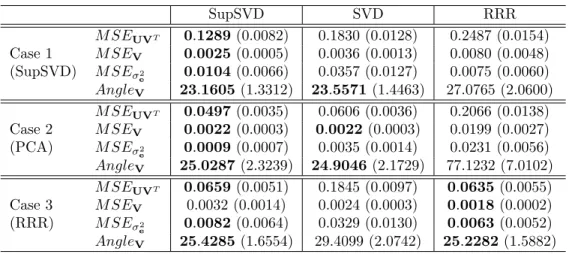
methods. The results clearly show that SupSVD performs favorably no matter which true model the data are generated from, while SVD and RRR only work well in their respective settings. This demonstrates that SupSVD, covering SVD and RRR as special cases, adapts to a wide range of practical situations. In practice, whenever additional information is available (whether it is truly supervision or not), SupSVD is always a good choice for dimension reduction. In these simulations, SupSVD always provides the best results, equivalent to (or better than) the method corresponding to the true data generative model.
SupSVD SVD RRR
M SEUVT 0.1289 (0.0082) 0.1830 (0.0128) 0.2487 (0.0154)
Case 1 M SEV 0.0025 (0.0005) 0.0036 (0.0013) 0.0080 (0.0048)
(SupSVD) M SEσ2
e 0.0104 (0.0066) 0.0357 (0.0127) 0.0075 (0.0060)
AngleV 23.1605(1.3312) 23.5571 (1.4463) 27.0765 (2.0600)
M SEUVT 0.0497 (0.0035) 0.0606 (0.0036) 0.2066 (0.0138)
Case 2 M SEV 0.0022 (0.0003) 0.0022 (0.0003) 0.0199 (0.0027)
(PCA) M SEσ2
e 0.0009 (0.0007) 0.0035 (0.0014) 0.0231 (0.0056)
AngleV 25.0287(2.3239) 24.9046 (2.1729) 77.1232 (7.0102)
M SEUVT 0.0659 (0.0051) 0.1845 (0.0097) 0.0635(0.0055)
Case 3 M SEV 0.0032 (0.0014) 0.0024 (0.0003) 0.0018(0.0002)
(RRR) M SEσ2
e 0.0082 (0.0064) 0.0329 (0.0130) 0.0063(0.0052)
AngleV 25.4285(1.6554) 29.4099 (2.0742) 25.2282 (1.5882)
Table 2.1: Median(MAD) for Low Rank Structure Recovery Accuracy and Parameter Esti-mation Accuracy.
Note that Table 2.1 also shows that the M SEV of SupSVD is larger than the other two methods when the data are generated from the RRR model, i.e. in Case 3. We remark that this is due to the low identifiability of the SupSVD model when the trueΣf is exactly zero. Numerically, SupSVD is still applicable but the estimated loading vectors are subject to an unstable orthogonal rotation. However, we comment that the estimated projection subspace of V (i.e., AngleV) and the low-rank recovery accuracy (i.e., M SEUVT) are unaffected.
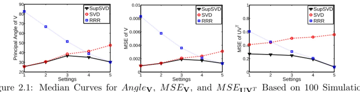
2.5.1.2 Comparison across A Spectrum
We now compare SupSVD, SVD and RRR across a spectrum of simulation settings ranging from the PCA model to the RRR model. For easy presentation, we set n = 210, p = 68,
q = 1, and r = 1. Fill the 210×1 vector Y with standard normal random numbers. We simulate X from the SupSVD model, with the loading vector being the first column of V in Case 1 above,σ2e = 16, and (B,Σf) ∈ {(0,36),(1,25),(2,16),(3,9),(4,0)}, corresponding to Setting 1 to 5, respectively. Therefore, the SupSVD model ranges from the PCA model X = 6ZVT +E (Setting 1; Z is a random vector with i.i.d. entries from standard normal distribution) to the RRR modelX= 4YVT +E (Setting 5). Again, under each setting, we run 100 simulations and summarize the results.
To avoid redundancy, we only show the median curves ofM SEUVT,M SEV, andAngleV
for the methods in Figure 2.1. We observe that SupSVD is uniformly the best over the spectrum of settings, with similar performance with SVD when the true underlying model is PCA, and similar performance with RRR when the true underlying model is RRR. Again, the results illustrate that SupSVD is a robust method that adapts well over a wide range of data-generating models.
1 2 3 4 5
20 30 40 50 60 70 80 90 Settings
Principal Angle of V
SupSVD SVD RRR
1 2 3 4 5
0 0.002 0.004 0.006 0.008 0.01 Settings
MSE of V
SupSVD SVD RRR
1 2 3 4 5
0 0.2 0.4 0.6 0.8 1 Settings MSE of UV T SupSVD SVD RRR
Figure 2.1: Median Curves for AngleV, M SEV, and M SEUVT Based on 100 Simulation
Runs.
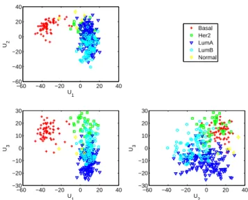
2.5.2 Breast Cancer Data
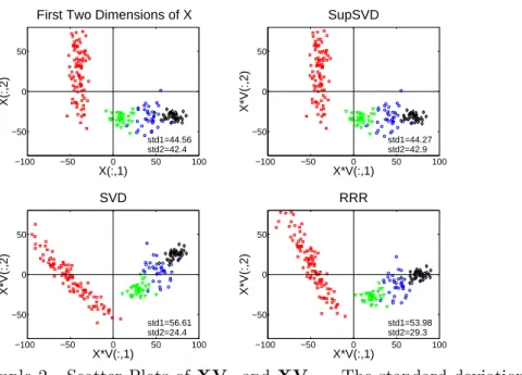
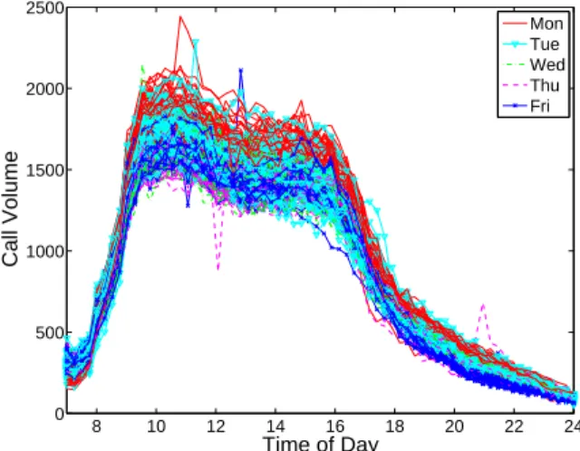
We consider a real data set containing gene expression measurements from breast tumors, obtained from the The Cancer Genome Atlas (TCGA) project (The Cancer Genome Atlas Network, 2012). A pointer to the publicly available data is athttps://tcga-data.nci.nih.
of genetic variation among tumors. In this case, we have additional information of disease subtype for each tumor. We may regard cancer subtypes as a partial driver of the underlying structure of the gene expression data (Schadt et al., 2005). Samples from the same subtype will share common genetic variations. We use the subtype information as our supervision data and apply the SupSVD method.
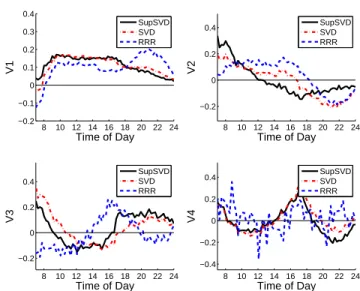
The raw data set contains 17814 genes and 348 samples. Out of the 348 samples, there are 5 subtypes of breast cancer with different number of samples in each subtype: Basal (66), Her2 (42), LumA (154), LumB (81), and Normal (5). We preprocessed the data in the same way as in Lock and Dunson (2013). We first imputed missing values with the k-nearest neighbors algorithm (k= 10), then removed genes with low variations across samples (standard deviation smaller than 1.5), and finally mean centered each gene. The result is a column-centered data matrixX with 348 samples and 645 genes. Based on the scree plot of the singular values ofX, we select the rank of the underlying structure to be 3.
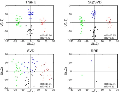
Figure 2.2 shows the scatter plots of the estimated SupSVD scores. The first score vector clearly separates the Basal subgroup from the rest. The second score vector captures vari-ations within each subtype. The third score vector roughly separates the Her2, LumA, and LumB subgroups.
−60 −40 −20 0 20 40
−60 −40 −20 0 20 40
U1
U2
−60 −40 −20 0 20 40
−30 −20 −10 0 10 20 30
U1
U3
−60 −40 −20 0 20 40
−30 −20 −10 0 10 20 30
U2
U3
Basal Her2 LumA LumB Normal
Genes
Samples
First Layer
200 400 600 50
100
150
200
250
300
Genes
Samples
Second Layer
200 400 600 50
100
150
200
250
300
Genes
Samples
Third Layer
200 400 600 50
100
150
200
250
300
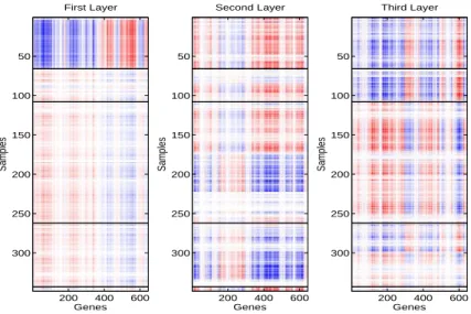
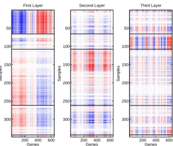
Figure 2.3: Breast Cancer Data - Heat Map of First Three Unit-rank SupSVD Structures of the Gene Expression Data. Blue is negative and red is positive. The samples are grouped in the order of Basal, Her2, LumA, LumB, Normal. The genes are reordered for better visualization.
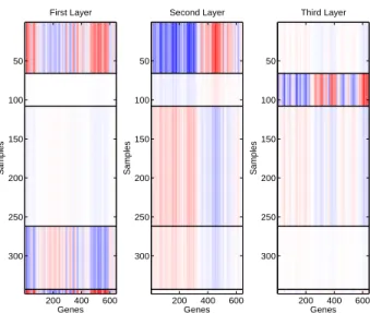
Figure 2.3 presents the heat maps of the unit-rank structures from SupSVD. There are clear patterns driven by subtypes. For example, the first layer is dominated by the unique pattern in the Basal subgroup. The third layer shows patterns similar between Basal and Her2, but different among Her2, LumA and LumB. There are also within-group variations that are not driven by subtypes. For example, the LumA samples in the second layer clearly exhibit several different patterns. The SVD and RRR results are given in the appendix, Section 2.7.7. In comparison, SupSVD effectively captures important underlying patterns consisting of both between-group variations driven by the subtype information and within-group variations from unknown sources.
2.6 Discussion
contains the PCA model and the RRR model as two extreme cases: when the supervision information is unrelated to the data of interest, SupSVD reduces to PCA; when the underlying structure is fully driven by the supervision information, SupSVD reduces to RRR. SupSVD automatically adjusts the amount of supervision used for dimension reduction without the use of tuning parameters. The proposed EMS algorithm for parameter estimation in SupSVD is computationally efficient. Asymptotic properties of SupSVD are derived for the resulting estimates. Simulation studies and real data applications clearly demonstrate the advantages and flexibility of the SupSVD method.
Dimension reduction is also useful in functional data analysis (FDA) to facilitate vari-ous subsequent analyses. For an overview of the FDA literature including recent advances, see Bongiorno et al. (2014); Ferraty and Vieu (2006); Horv´ath and Kokoszka (2012); Silver-man and Ramsay (2005). We remark that our SupSVD method can be directly adapted to FDA through a basis approach. In particular, one can decompose discretized observations of functional data onto proper basis functions, obtain a coefficient matrix, and then apply SupSVD to the coefficient matrix. The low rank approximation obtained from SupSVD can then be converted back to the original functional space through the basis functions. Another approach is to first select important variables in discretized values of the function (Aneiros and Vieu, 2014), and then apply SupSVD to the dimension-reduced vectors. Alternatively, in the next chapter, we extend the recent regularization formulation of functional principal component analysis (Huang et al., 2008, 2009) to incorporate supervision for FDA. We im-pose both sparsity (Shen and Huang, 2008b) and roughness regularization to incorporate both high-dimensional multivariate data as well as infinite-dimensional functional data.
2.7 Appendix
2.7.1 Proof of Proposition 2.2.1
Proof. Let (B,V,Σf, σ2e) be a parameter set such that B is a q×r matrix, V is a p×r
the rest p−r equal eigenvalues. It’s equivalent to say that VΣfVT has r positive distinct eigenvalues. We have the eigen-decomposition of thep×pmatrixVΣfVT as
VΣfVT =VbΣcfVbT
whereΣcf is the r×r diagonal matrix containing the distinct eigenvalues, andVb is thep×r orthonormal matrix containing the corresponding eigenvectors. Moreover, set Bb =BVTV.b SinceV and Vb have the same column space, we know
BVT =BbVbT.
Therefore, the new parameter set (Bb,Vb,Σcf, σ2e) is equivalent with the original parameter set in terms of Model (2.2), and satisfies the aforementioned identifiability conditions.
The uniqueness of the resulting parameter set is guaranteed by the uniqueness of the eigen-decomposition of the matrix with distinct eigenvalues.
2.7.2 Proof of Proposition 2.3.1
Proof. Letθ(i)= (B(i),V(i),Σ(fi), σe2
(i)
) denote the EMS parameter estimation from theith iteration. From the algorithm we know it satisfies the identifiability conditions. LetQ(θ|θ(i)) denote the conditional expectation of the joint log likelihood. Namely,
Q(θ|θ(i)) = EU(L(X,U|θ)|X,θ(i))
= EU(L(U|X,θ)|X,θ(i)) +L(X|θ)
Letbθ denote the unconstrained optimizer from the M step of EMS algorithm. Namely,
b
θ= arg max θ Q(θ|θ
Referring to the information inequality that Eg(logf) ≤Eg(logg) for any densities f and g,
we have
EU(L(U|X,bθ)|X,θ(i))≤EU(L(U|X,θ(i))|X,θ(i))
Combining with the fact Q(bθ|θ(i))≥Q(θ(i)|θ(i)), we know
L(X|bθ)≥ L(X|θ(i))
Moreover, letθ(i+1) denote the equivalent parameter set that satisfies the identifiability con-ditions. We have
L(X|θ(i+1)) =L(X|bθ)≥ L(X|θ(i))
Therefore, the likelihood of the observed data X is monotonically nondecreasing with itera-tions. If we assume the maximum likelihood exists, the EMS algorithm can always converge.
2.7.3 Details of Algorithm 1
In the paper, we propose the EMS algorithm, which is a modified version of EM algorithm, to efficiently estimate the SupSVD model parameters. The detailed calculations for each step in each iteration are described below. We use (B(i),V(i),Σ(i)
f , σe2 (i)
) to denote the estimations from the ith iteration.
Initial estimation: Our numerical studies indicate the algorithm is not sensitive to initial values. In practice, we apply SVD to the matrixXto get the initial estimation. More specifically, we first find the rank-r approximation ofX as
X≈UVT (2.17)
orthonormal columns (i.e., the submatrix of the right singular matrix). Here V is an initial estimation of V in our model. We treat X−UVT as a random matrix with i.i.d. entries from N(0, σe2). Therefore we can get an initial estimation of σe2. Then we regress U on Y and assume that the multivariate residuals are i.i.d. with diagonal covariance structure. The regression coefficient matrix is an initial estimation ofB and the diagonal covariance matrix is an initial estimation ofΣf.
E step: We have the conditional distribution (2.10) of U given X under the current parameter estimations. We can calculate the following quantities to be used in M step.
(1) First order conditional expectation:
EU
U|X, θ(i) =
YB
σ2e(i)Σ(fi)−1
+XV(i) Ir+σ2e (i)
Σ(fi)−1 −1
, Θ(Ui)|X
(2) Second order conditional expectation:
EU
UTU|X, θ(i)=nΩ(Ui)|X+ Θ(Ui)|XTΘ(Ui)|X
where Ω(Ui)|X,
Σ(fi)−1+σ−2 e
(i)
Ir
−1
.
(3) Conditional expectation of any quadratic form inU:
EU
tr U∆UT
|X, θ(i)=ntr∆Ω(Ui)|X+ tr
Θ(Ui)|X∆Θ(Ui)|XT
where∆is anyr×r symmetric matrix.
M step: We maximize the object functionEU L(X,U)|X, θ(i)