Alexandros Christodoulou
A thesis submitted to the faculty of the University of North Carolina at Chapel Hill in partial fulfillment of the requirements for the degree of Master of Arts in the Department of Psychology
Chapel Hill 2009
Abstract
Alexandros Christodoulou: Thinking Prosody: How speakers indicate production difficulty through prosody
(Under the direction of Jennifer E. Arnold)
Acknowledgements
First and foremost, I would like to thank my advisor Dr. Jennifer E. Arnold for her intermittent guidance from the conception to the completion of this research project.
Table of Contents
List of Tables...vi
List of Figures...vii
Chapter I. Introduction...1
II. Evidence for Thinking Prosody...7
Latency to begin speaking...7
Longer word duration...9
Frequent pausing...10
Higher pitch...10
III. Experiment 1...12
Method...13
Participants...13
Equipment...13
Materials...13
Procedure...15
Disfluency analysis...17
Acoustic analysis...18
Discussion...19
IV. Experiment 2...22
Method...26
Participants...26
Materials...26
Procedure...29
Results...29
Primary analysis...32
Secondary analysis...34
V. General Discussion...38
List of Tables
Table
1. Conditions in Ferreira and Swets (2002)...8
2. Critical Regions in Utterance...17
3. Experiment 1: mean duration for all regions in utterance...18
4. Experiment 1: average Pitch for all regions in utterance...19
5. Experiment 2: disfluency rate in target region...31
6. Experiment 2: average number of words in target region...32
7. Experiment 2: average log duration of color word for all conditions...33
8. Experiment 2: average pitch over color word for all conditions...33
9. Experiment 2: average Maximum Pitch over Color Word for all conditions...34
10. Experiment 2: average Minimum Pitch over Color Word for all conditions...34
11. Experiment 2: average log duration of color word for all conditions...35
12. Experiment 2: average pitch over color word for all conditions...35
13. Experiment 2: average Maximum Pitch over Color Word for all conditions...35
List of Figures
Figure
1. Example of disfluent interaction from the Fisher Corpus...2
2. Typical experimental items in experiment 1...14
3. Experimental Conditions in experiment 2...27
Introduction
Speakers can carry on conversations in what seems to be a fairly automatic way. Nevertheless, the production process is not resource free. The speaker needs to go
through a discrete set of steps in order to formulate their final utterance. Once the speaker formulates his or hers communicative intention, he or she needs to translate that into words, put the words in order, and then pronounce them (Bock, 1982; Bock 1995). In addition, each step poses different resource demands on the processing system. The more complicated the message, the more resource intensive the production process will be, and thus the more disfluent the speaker will be (Bortfeld, et al. 2001).
yeah i i kind of agree i i don't
i don't i don't i don't easily foresee the situation where i would
you know either be asked to or know something or you know you know
i've never
been in that position where i've you know been asked to
Figure 1. Example of disfluent interaction from the Fisher Corpus. The indentation before each line and the spaces between words represent a significant pause in the speech stream.
The example is taken from the Fisher Corpus (Cieri, et al. 2004) and it represents a conversation turn of two people talking about a predetermined topic over the phone. The topic is “would you commit perjury” and the speaker, seems to be experiencing a great deal of difficulty to answer the question. This is probably because hei has never been asked that question before and he is struggling to frame his communicative intention (Chafe, 1974). However, production difficulty doesn’t only lead to disfluencies, it also leads to modulations in sentence prosody.
Longer latency to begin speaking and pausing are evident in the example from the Fisher corpus. In addition, the speaker might also lengthen word duration and implement a high pitch excursion. All of these acoustic effects are part of sentence prosody. In brief, prosody consists of all the acoustic elements that create the metric and rhythmic pattern of a sentence. They generally include measures of duration, pitch and intensity.
Research in language comprehension suggests that prosody carries information about production difficulty that can be utilized by the listener. Arnold et al. (2004) has shown that listeners take advantage of disfluency in order to speed up their
comprehension process. When the listener hears a disfluency he or she is more prone to look faster at an unfamiliar pictured referent compared to a familiar pictured referent. For example, when the listener sees a picture of a car and a picture of an abstract linear composition, he or she is more prone to look at the abstract picture as soon as they hear a disfluency. However, when Arnold and Tanenhaus (in press) manipulated the
pre-disfluency prosody, they found that listeners were significantly faster at looking at the abstract picture only when the disfluency is preceded by longer duration and higher pitch excursion. This finding suggests that the speaker’s prosody can carry information about production difficulty, in addition to disfluency.
Research on sentence prosody nonetheless usually studies it in relation to linguistic structure. For example, linguistic contrast is a well-documented factor that modulates prosody (Hirschberg & Pierrehumbert, 1986;Pierrehumbert & Hirschberg, 1990). Linguistic contrast is implemented when the linguistic context activates a set of
alternatives the speaker needs to choose from (Bolinger, 1986; Chafe, 1974). If there are two cars, blue and red, in plain view to the speaker, the speaker will refer to the BLUE car in an acoustically prominent way; most probably with higher pitch, longer duration and higher intensity.
individual features, such as duration. For example Ferreira and Swets (2002) manipulated the computational difficulty of an addition problem and measured latency to begin
speaking and word duration. In this type of experimental design duration represents mental processing time. In a similar manner research on disfluency has analyzed the length of the pause before a lexical repair as the amount of time required to mentally prepare for the repair (i.e. Levelt, 1984).
Overall prosody is sensitive to both linguistic structure and language production processes. Both of these factors affect the acoustic components of prosody in a specific way. In this masters thesis I try to integrate these two lines of research in order to show that production difficulty affects sentence prosody, in addition to disfluencies. In order to show this I will measure acoustic elements such as duration and pitch. This way I can capture the effects of processing on the message through analyzing all the acoustic features associated with sentence prosody.
Arnold and Tanenhaus (in press) manipulated prosody specifically for the purpose of their comprehension experiment. They termed the prosodic manipulation Thinking Prosody because it sounded like the speaker was thinking. Thinking prosody consisted of longer word duration and higher pitch excursion over the area before the critical
studied before in conjunction with production research. This is because most researchers would look at the critical description area for disfluencies. Moreover, research on
disfluencies has not found any evidence for pre-disfluency prosody (i.e. Nakatani & Hirschberg, 1994).
The main topic of interest of this thesis is thinking prosody. I hypothesize that thinking prosody is composed of the following acoustic features: longer latency to begin speaking, longer word duration, frequent pausing, higher pitch excursion. Even though the concept of thinking prosody comes from Arnold and Tanenhaus (in press), their manipulation was for a comprehension experiment. Therefore, their results don’t show that thinking prosody is a naturally occurring behavior. It is still unknown whether speakers produce thinking prosody and what the exact component acoustic features are. Of particular interest is to find evidence of pitch excursion as part of thinking prosody. Even though pitch is highly sensitive to semantic and pragmatic factors, it hasn’t been linked with language production factors yet. Most importantly, the combination of acoustic features over a segment of an utterance hasn’t been studied in conjunction with production difficulty.
Chapter 2
Evidence for Thinking Prosody
The main hypothesis for thinking prosody is that it will consist of an increase in frequency of pausing and in measures of pitch and duration, as compared to fluent delivery. Therefore, I expect: longer latency to begin speaking, longer word duration, longer and more frequent pausing, and higher pitch measures. These features will all precede the area of description of a difficult to describe referent, as in Arnold and Tanenhaus (in press). In the rest of this section I review evidence for each acoustic segment proposed under the thinking prosody hypothesis.
The association of processing time and duration measures is well established in the production literature. Previous research has looked at: the amount of time it takes to start speaking, word duration and length of pausing. All of these measures are predicted to be part of thinking prosody.
Latency to begin speaking
Speakers tend to take longer to start an utterance when experiencing production difficulty (Ferreira & Swets, 2002; Griffin, 2003). Ferreira and Swets (2002) manipulated the difficulty of addition problems and asked participants to verbalize the result by
each condition. Difficulty was manipulated in both the ones and the tens digits of the sum. If the sum of the ones or the tens were higher than 5, that unit was considered difficult.
Table 1
Conditions in Ferreira and Swets (2002)
Ones Tens Addition Sum
Easy Easy 21 + 22 = 43 >5, >5
Easy Hard 21 + 26 = 47 >5, <5
Hard Easy 21 + 62 = 83 <5, >5
Hard Hard 21 + 66 = 87 <5, <5
They found that the speakers didn’t start speaking until they had solved the whole problem. They therefore took longer to begin speaking in the harder condition compared to the easier condition. However, when the experimenters asked them to start speaking as soon as they saw the problem, they still took longer to begin speaking compared to the easy condition but not as long as without a time limit.
This result shows that speakers take a flexible approach to pausing before initiating speech; they only pause if they can’t allow for processing time during speech.
These studies taken together (Griffin, 2003; Ferreira & Swets, 2002) provide support to the idea that higher production difficulty leads to a longer latency to begin speaking. The respective difficulty might be due to longer expected articulation time as well as longer expected conceptualization time. Therefore, these results suggest that different levels of message composition can have an effect on latency to begin speaking. Longer word duration
Ferreira and Swets (2002) also provide evidence that word duration lengthens under conditions of planning or processing difficulty. When the tens of the sum were difficult the carrier phrase was shorter, however when the ones were difficult the carrier phrase was longer. These results are in line with the idea that the speaker will lengthen words in order to deal with upcoming difficulty. Arnold et al. (2007) also provide evidence for length. In a production experiment they asked participants to describe pictures and found that the area before the target description had a longer duration in the unfamiliar
Frequent pausing
Evidence for pausing associated with production difficulty comes mainly from the disfluency literature. According to Levelt (1983, 1989) a pause of at least 200ms is needed in order to plan a new utterance. Clark and Wasow (1998) argue that speakers pause before complex constituents and Watson and Gibson (2005) argue that the
probability of a pause increases as the constituent becomes more complex. The degree of production difficulty should therefore modulate the frequency of pausing during
production.
Pitch is also predicted to be part of thinking prosody. Even though the production literature has not established a direct relationship between production difficulty and higher pitch, the motivation to include pitch comes from the explicit manipulation of pitch excursion in the pre-disfluency region by Arnold and Tanenhaus (in press). Higher pitch
Chapter 3 Experiment 1
Experiment 1 was conducted in order to establish that production difficulty leads to thinking prosody. Of particular theoretical importance was to establish the connection between heightened pitch and cognitive load. Past research in the disfluency literature would predict higher pitch only during certain types of disfluencies (Shriberg, 1999; Levelt & Cutler, 1983). Levelt and Cutler have argued that the effects of pitch are due to “accenting” and not an increase in cognitive load. On the other hand the results from the feeling of knowing literature indicate that a longer mental search time will correlate with higher pitch.
Method Participants
Eight pairs of undergraduate students at UNC Chapel Hill enrolled in introduction to Psychology participated in exchange for credit towards their experimental credit class requirement. All were native speakers of English with normal or corrected to normal vision and normal hearing.
Equipment
I recorded the set of utterances in .wav format on a Marantz professional audio recorder over an Audio Technica professional microphone headset. I then used an iMac computer in order to store and analyze the sound files. For the stimulus presentation I used the Exbuilder software (Longhurst, 2006) running on two IBM computers, a desktop and a laptop. The laptop was connected to a set of speakers in order to amplify the sound that signaled the beginning of each trial.
Materials
Figure 2. Typical experimental items in experiment 1. The pictures to the left of the dark vertical line are one item with a familiar target. The pictures to the right of the dark vertical line are one item with an unfamiliar target. The gray square highlights the target. Pictures of the same color were always next to each other on the horizontal axis.
The competitor picture was always the same color and on the same horizontal axis as the target, but it had the opposite familiarity value (i.e. the competitor was familiar when the target was unfamiliar and vice versa) as in figure 2. I used eight colors; red, blue, green, yellow, brown, black, orange, purple. The role of the distracters was to introduce two pairs of the same color. This way the speaker would have to say the color word in order to uniquely identify the referent. For example when referring to figure 2, you can’t just say: “click on the apple”. They were the exact same set of pictures as the target and the competitor, but in a different color. In other words if the target and competitor were a familiar and an unfamiliar item in blue, then the distracters were a replication of the same picture set in orange. I treated picture position and color as a control variable and then counterbalanced across trials.
There were also 24 fillers in order to minimize sequence effects. If I were to present the speakers with 24 stimulus trials, chances are the speakers would start anticipating a comparison between a familiar and an unfamiliar item. The filler trials had the same layout as the stimuli, however each trial consisted of all familiar or all unfamiliar
pictures. Therefore, the speakers would also need to compare among familiar pictures and among unfamiliar pictures.
Procedure
describe the highlighted pictured so that the listener could identify it on his or her screen. The trial started when I said go. Then the participants clicked on a black dot in the middle of the screen and immediately saw the four pictures. As soon as the speaker heard a beep sound he or she would start describing the highlighted picture. At the same time, the listener had no information as to which picture was highlighted. I asked the speaker to use the carrier phrase “click on the color” when describing the target. A typical utterance in the familiar condition sounded like: “click on the orange apple.
The role of the listener was to identify the described object on his or her screen according to the speaker’s description. As soon as the description was over, the listener clicked on the target picture in order for the black dot to appear again. As soon as the listener identified the correct referent by clicking on the picture, the black dot appeared on their screen as well. In order to ensure both speaker and listener maintained the same pace, I asked them to wait until the experimenter said go so both of them could click on the black dot at the same time and initiate the new trial.
Results
further analysis in order to avoid measuring prosodic effects of disfluencies (n=85, one pair was not analyzed because the speaker kept saying “the picture of” after “click on”). In a number of cases the speakers preferred to describe the target first and then the color. The directions required them to say the color first and then the target. These cases were also excluded from further analysis (n=24). Any other instances where the speaker made a mistake during the utterance by omitting or changing some of the required information, or where the speaker wasn’t able to identify the right referent, were omitted (n=11). The remaining utterances (n=93) were submitted to acoustic analysis.
For the acoustic analysis the following regions in the utterance were identified: latency to begin speaking, click on, the, interval, color, interval, target. Table 2 depicts the respective regions. I measured length, average pitch and pitch excursion for regions 2,3,5 (see table 2). I conducted the measurements with the aid of two scripts for the praat speech analysis software (Boersma, Weenink, 2008) authored by Katherine Crosswhite.
Table 2.
Critical Regions in Utterance
1. Latency 2. Click on 3. The 4. Interval 1 5. Color 6. Interval 2 7. Target
Click on The Pause Red Pause Couch
Latency refers to the region between beep and beginning of utterance
Disfluency analysis
condition as indicated by a higher disfluency rate and a larger number of words. A total of 93 responses from seven speakers were analyzed. A one way repeated measures ANOVA revealed that disfluencies were significantly more frequent in the unfamiliar condition by subjects, F1(1,5)= 15.06, p<0.05. Also, the unfamiliar condition showed a significantly greater number of words in the target region, F1(1,5)=11.5, p<0.05.
Acoustic analysis:
The results show longer duration in the pre-target region in the unfamiliar
condition compared to the familiar condition, as well as a higher average pitch range over the color word. Table 3 presents the mean duration (ms) for the different conditions: Table 3.
Experiment 1: Mean duration for all regions in utterance Familiar
Familiar UnfamiliarUnfamiliar
Region Mean Std Dev Mean Std Dev
1. Latency 756.94 219.13 921.92 272.27
2. Click on 414.06 106.18 507.88 136.06
3. The 202.90 128.28 301.00 158.29
4. Interval 1 63.65 90.40 205.74 254.57
5. Color 290.63 150.48 478.63 231.00
6. Interval 2 137.71 259.54 385.06 599.84
Duration: A one way repeated measures ANOVA revealed that the participants took significantly longer to say “click on” in the unfamiliar condition, F1(1,5)=7.7, p<0.05; F2(1,22)=16.4, p<0.01, and to say the color word, F1(1,5)=12.2, p<0.05; F2(1,22)
=16.56, p<0.01. They also paused significantly longer in the unfamiliar condition
The main effect of familiarity on duration approached significance in the rest of the segments. The participants took significantly longer to start their utterance by subjects F1 (1,6) = 3.92, p<0.1, and only marginally longer by items F2 (1,22)=14.7, p<0.1, they
took longer to say “the” only by items F2(1,22)= 4.4, p<0.05, but not by subjects F1(1,5) = 1.44, p>0.05.
Table 4.
Experiment 1: Average Pitch for all regions in utterance Familiar
Familiar UnfamiliarUnfamiliar
Region Mean St Dev Mean St Dev
3. Click on 207.66 14.88 207.35 17.99
4. The 190.19 11.82 188.78 14.29
6. Color 188.53 13.38 195.86 13.63
Pitch: A one way repeated measures ANOVA revealed that the participants had a
significantly higher average pitch in the color region of the unfamiliar condition, F1 (1,5) =7.9, p<0.05, F2 (1,20)= 6.7, p<0.05.
Discussion
The acoustic analyses from experiment 1 verified our predictions. They reveal that when speakers are facing an increase in production difficulty they tend to elongate their words, pause more frequently and produce a higher average pitch. All these
What is more, thinking prosody cannot be solely considered a byproduct of disfluency.
Researchers who investigate disfluency have been mostly concerned with the role of prosody during the disfluent region (i.e. Shriberg, 2001). Even more, computational linguists have been mostly concerned with acoustic characteristics of disfluency that can aid speech recognition models to predict disfluency (i.e. Nakatani and Hirschberg, 1994). Our results are complementary to those efforts and can shed new light on the function of prosody. The combination of results from these types of research can possibly show what a flexible medium prosody is. Over the disfluent region, prosody can carry information about metalinguistic aspects such as a warning sign that the speaker has committed a speech error and they are about to correct it (Levelt & Cutler, 1983). What is more, prosody can be the sole carrier of the processing difficulty that is usually carried by disfluencies.
An important result of experiment 1 is that the color word receives acoustic prominence, in the form of longer duration and higher pitch. This suggests that
Chapter 4 Experiment 2
The purpose of the second experiment is to examine the relationship between thinking prosody and accenting. In the introductory section I described thinking prosody as a host of prosodic features. Furthermore, the results of experiment 1 suggest that an increase in cognitive load can lead to acoustic prominence. Speakers usually experience an increase in cognitive load when producing new information in the utterance or when they describe something unfamiliar. Speakers also use acoustic prominence when accenting information. They show more pitch movement, segmental lengthening and higher intensity (Bolinger, 1986). This type of acoustic prominence might be similar to acoustic prominence under production difficulty. Moreover, production difficulty is often confounded with discourse status. Whatever is new in the discourse is also usually more difficult to produce because it is less accessible. This suggests there might be
types of prominence depend on each other to a certain degree. However, a lack of interaction might indicate that the two types of accenting are acoustically different.
Speakers usually accent information in order to implement linguistic focus (Bolinger, 1986, Terken & Nooteboom, 1987). Linguistic focus refers to the way information stands out in relation to the linguistic context. For example narrow focus is usually given only a contrastive interpretation (Ladd, 1980) and is usually perceived as being accented. The following gives an example of contrastive focus: click on the RED apple. The color word is capitalized in order to indicate its acoustic prominence over the
rest of the utterance. This type of focus indicates to the listener there is an alternative referent that contrasts along a specific dimension with the actual target. Therefore it is also known as contrastive accent.
Speakers also might accent information in order to denote the degree of accessibility of discourse information. Interlocutors usually track the information introduced by an utterance in the form of discourse entities. The recency of the mention of a discourse entity determines its degree of activation. When the information is already mentioned in the discourse it will most probably be de-accented (Fowler & Housum, 1987). For example if a speaker has already referred to a red apple, the color adjective and the noun will most probably be acoustically attenuated. However, when the
information is new to the discourse it will most probably receive an accent (Chafe, 1974). The speaker will thus experience a possible increase in cognitive load because new information is less accessible.
accenting, we need to create an experimental design where contrast is not confounded with production difficulty.
Gregory et al. (2003) manipulated the type of pre-nominal modifier in order to implement different types of contrast. Two people participated in the task. The one
participant gave directions to the other participant to move a certain object that contrasted with another object in one of three different dimensions: scale, material and color. For example if there were two cups on the grid and they contrasted on scale, the director would ask the other participant to move the TALLER cup. They counted the number of disfluencies immediately before the pre-nominal modifier in order to measure the amount of production effort imposed on the speaker when producing different types of contrast. They found that there is no significant difference in disfluency rate in the no contrast vs. contrast condition for color words. This means that if the director is asking the other participant to move the RED cup when there is also a blue cup on the grid, the director will not experience an increase in cognitive load.
Krahmer and Swerts (2001) argue that even though contrastive accents tend to be judged as perceptually more salient compared to newness accents (e.g. when the
participant would say “blue triangle”. The shapes and the colors were selected to create four different types of contrast conditions: All new information (no contrast), color contrast, noun contrast and double contrast. The first mentioned object was always
considered new information. Objects mentioned later in the task could carry either a color contrast, or a noun contrast depending on the element of the object that was being
contrasted with the previously mentioned object. Lastly, double contrast was implemented when the current object contrasted on both elements of the previously mentioned object. The experimenters conducted an intonational analysis on the material and found that there was no difference between the type of intonation used in the all-new condition and the other types of contrast. As far as the distribution of accenting is
concerned they found that the speakers accented only the contrasting item. For example, in the color contrast condition the speaker would accent only the color and not the noun.
In the second experiment I use a contrastive environment (as in Krahmer & Swerts, 2001) with color words in order to avoid increasing cognitive load during production (Gregory et al., 2003). Therefore, this experimental design can help identify the
Method Participants
18 pairs of undergraduate students at UNC Chapel Hill enrolled in introduction to Psychology participated in exchange for course credit. All were native speakers of English with normal or corrected to normal vision and normal hearing.
Materials
I used the same set of equipment as in experiment 1. I manipulated cognitive load by varying picture familiarity as in experiment 1. For the experimental materials I used a subset of the pictures from experiment 1 and generated 24 trials. I presented four pictures at the same time, however I held familiarity constant for the pictures in each trial.
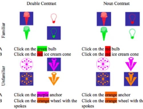
Figure 3. Experimental Conditions in experiment 2. The blue shading highlights the target. Each item had two targets. The second target appeared only after the first target had been described. The color and object type of the first target in comparison to the second target determined the type of contrast.
condition both picture and color for the targets were different. For example the first target was a green light bulb and the second target a red ice cream cone.
In order to reduce the sources of variability in the prosody of the sentence I used only 4 colors: red, green, orange and purple. Red was always paired with green and orange was always paired with purple in order to control for number of syllables. In other words each trial could have two color configurations: red – green, or orange – purple, which were counterbalanced across trials. I also held the target color and position constant and counterbalanced across trials.
I treated contrast as a within subjects variable. Therefore I generated three conditions for each stimulus trial. I held the second target for all conditions constant and changed the first target according to contrast condition. In order to counterbalance the conditions without repeating items, I used a Latin square design as in experiment 1. This generated three different lists of 24 items that the participants were randomly assigned to. The lists were also counterbalanced across participants.
The experimental design resulted in six different conditions. However the
statistical analysis will be conducted in two stages. The first analysis will include 2 levels of the contrast variable: double and noun, and the two levels of the familiarity
manipulation: familiar and unfamiliar. A second analysis will include only two levels of the contrast manipulation: color and noun in the familiar condition. This analysis
any of the statistical analyses, because the speaker needs to repeat the same unfamiliar picture twice. Therefore, the picture will not be unfamiliar anymore during the second mention. The reason this condition is included in the design is because it acts as a filler and it also balances the familiar and unfamiliar items. The following figures depict the familiar and unfamiliar color contrast conditions.
Figures 4 a and b. Manipulation check. The picture on the left represents the familiar color contrast condition. This condition is compared to the familiar noun contrast condition. The picture to the right refers to the unfamiliar color contrast condition. This condition serves as a filler.
Procedure
I used the same procedure as in experiment 1 with the exception that the speaker described two targets in succession. In the beginning of the trial one of the pictures was highlighted. As soon as the listener identified the right referent, the second picture was highlighted (see figure 3). I made sure that the speaker waited for the listener to identify the object within each experimental trial as well as between trials.
Overall there were 18 pairs of participants, 5 of which were excluded. Pair two was excluded because the speaker kept referring to the red pictures as pink. The speaker in pair five mentioned she was trying not to use accenting because she wanted to make the task harder for the listener. The recordings for pairs six and twelve had poor sound quality and the speaker of pair ten was colorblind.
The data of the remaining 13 pairs were transferred to a Macintosh computer and transcribed, following the same conventions used for experiment 1. The speakers implemented their contrast during the second utterance. Therefore I only analyzed data from the second utterance. I also used the same exclusion criteria; I excluded any utterances with disfluencies before the color word. I also excluded items where the speakers mentioned the target description before the color word. Furthermore I excluded utterances with poor sound quality or extraneous background noises. This procedure led to an exclusion of 25 utterances. Overall I analyzed 287 utterances.
For the acoustic analysis I identified the color word as the area of interest. I am only interested in the color word because that’s the only region I can directly compare the effects of contrast to that of production difficulty. According to Krahmer and Swerts (2001) the contrasting item is the only one being accented. I measured word length, average pitch, maximum pitch, minimum pitch, pitch excursion and intensity. I conducted all acoustic analysis using the same praat scripts from experiment 1.
contrast condition (as shown in Figure 3).
Disfluency analysis
Speakers showed an increase in disfluency rate and an increase in number of words in the target region in the unfamiliar conditions. This shows that the speakers experienced an increase in cognitive load when describing an unfamiliar picture. This is also
consistent with results from experiment 1. Even more, speakers did not produce a higher rate of disfluency in the no contrast compared to the contrast condition. This replicates the findings by Gregory et al. (2003).
I conducted a 2 X 2 repeated measures ANOVA with disfluency rate and number of words as the dependent variables. There was a main effect of familiarity on disfluency rate F1(1,190) =25.27, p<0.0; F2(1,22.8) =13.31,p<0.05. There was also a main effect of familiarity on number of words in the target region F1(1,26.2) =45.15, p<0.01; F2 (42,37)= 42.37, p<0.01. There was no main effect of contrast on disfluency rate F1
(1,190)=0.03, p=0.8671; F2(1,181)=0.01, p=0.943.1.
Table 5.
Experiment 2: disfluency rate in target region
Condition Condition
Familiarity Double Contrast Noun Contrast
Familiar 0.9% 0.8%
Table 6.
Experiment 2: average number of words in target region
Condition Condition
Familiarity Double Contrast Noun Contrast
Familiar 1.27 1.22
Unfamiliar 3.27 2.79
Primary analysis
I analyzed both duration and pitch measures. For duration I expected the unfamiliar condition to show longer duration compared to the familiar condition. I also expected the double contrast condition to show longer duration compared to the noun contrast
condition. For pitch I expected average pitch and maximum pitch over the color word to be higher in the double contrast condition compared to the noun contrast condition. This result would show that speakers heighten their pitch in order to indicate linguistic
contrast. In order to replicate the previous finding of higher average pitch associated with production difficulty, I expected average pitch to be higher in the unfamiliar compared to the familiar condition.
169) = 1.19, p = 0.45; F2(1, 159) = 1.19, p = 0.28, and no significant interaction of
familiarity with contrast condition, F1(1, 170) = 0.91, p =0.34; F2(1, 159) = 1.67, p=0.20.
Pitch: I measured average pitch, minimum pitch, maximum pitch and pitch excursion and conducted a 2 X 2 ANOVA for each dependent variable.
Overall, there was marginal support for the hypothesis that speakers would use higher pitch when describing unfamiliar referent. There was a main effect of familiarity on average pitch by subjects but not by items, F1(1,167) = 6.90, p<0.01; F2(1,24.4) = 1.70, p = 0.2041. There was a main effect of familiarity on maximum pitch only by
subjects but not by items, F1(1,170) = 4.09, p<0.05; F2(1.166) =1.14, p=0.29. Table 7.
Experiment 2: average log duration of color word for all conditions
Double Contrast Noun Contrast
Mean St Dev Mean St Dev
Familiar 2.48 0.14 2.48 0.11
Unfamiliar 2.67 0.18 2.71 0.16
Table 8.
Experiment 2: average pitch over color word for all conditions
Double Contrast Noun Contrast
Mean St Dev Mean St Dev
Familiar 169.63 51.52 167.5 48.33
Table 9.
Experiment 2: average Maximum Pitch over Color Word for all conditions
Double Contrast Noun Contrast
Mean St Dev Mean St Dev
Familiar 176.60 54.18 176.15 51.25
Unfamiliar 182.13 54.81 183.84 53.95
Table 10.
Experiment 2: average Minimum Pitch over Color Word for all conditions
Double Contrast Noun Contrast
Mean St Dev Mean St Dev
Familiar 162.58 50.39 158.81 47.26
Unfamiliar 164.34 50.49 164.18 48.77
Secondary Analysis
I conducted a secondary analysis in order to make sure the contrast manipulation was effective. I conducted a one way ANOVA with contrast as the only factor. The primary 2 X 2 ANOVA did not produce reliable statistics that the double contrast
condition produced higher acoustic measures compared to the noun contrast condition. A main effect of contrast in the secondary analysis will show if the color contrast condition produces reliably higher acoustics compared to the noun contrast condition. The
Table 11.
Experiment 2 secondary analysis: average log duration of color word for all conditions
Color Contrast Noun Contrast
Mean St Dev Mean St Dev
Familiar 2.47 0.10 2.49 0.11
Table 12.
Experiment 2 secondary analysis: average pitch over color word for all conditions
Color Contrast Noun Contrast
Mean St Dev Mean St Dev
Familiar 170.48 54.36 167.5 48.33
Table 13.
Experiment 2 secondary analysis: average Maximum Pitch over Color Word for all conditions
Color Contrast Noun Contrast
Mean St Dev Mean St Dev
Familiar 178.63 56.05 176.15 51.25
Table 14.
Experiment 2 secondary analysis: average Minimum Pitch over Color Word for all conditions
Color Contrast Noun Contrast
Mean St Dev Mean St Dev
Discussion
The results of experiment 2 are not conclusive about the relationship between thinking prosody and contrastive accenting. However, they are consistent with the effects of production difficulty on duration that were observed in experiment 1, and offer some additional limited support to the effects of production difficulty on pitch.
The effect of contrast on pitch was only marginal. This could be due to individual differences in the way the speakers accented information for linguistic contrast. Speakers can use different types of pitch curves in order to indicate accenting. They can start off from a low pitch at the beginning of the word and reach a maximum towards the stressed part of the word. Or, they can start off from a maximum pitch at the beginning of the word and reach a minimum towards the stressed part of the word. If speakers were using both of these strategies in experiment 2 then there should be no main effect of contrast condition on our pitch measures in our data. This is because the effect of individual variability might be stronger compared to the effect of contrast.
Chapter 5 General discussion
The combined results from the two experiments suggest that thinking prosody is a natural reaction to production difficulty. Moreover, they suggest that production difficulty affects the immediately preceding word, up to the beginning of the utterance. Speakers lengthen their words and pause more frequently from the beginning of an utterance that has an unfamiliar referent. Nevertheless, the idea that thinking prosody can partly explain acoustic effects of linguistic accenting is still open for debate.
areas map onto the underlying cognitive processing during production. For example Levelt (1983) claimed that speakers can start repairing a segment only after an interruption point. Further research showed that speakers can start planning a repair before even the point of interruption (Blackmer and Mitton, 1991). Our results show that speakers don’t necessarily need to resort to repairing their utterance if they handle difficulty right from the beginning of the utterance. This also shows that speakers can effectively maintain a message representation while “thinking on their feet”.
References
Almor, A. (1999). Noun-phrase anaphora and focus: The informational load hypothesis. Psychological Review, 106(4), 748-765.
Arnold, J. (1997). Reference form and discourse patterns. Unpublished PhD, Stanford, Arnold, J. E. (2008). Reference production: Production-internal and addressee-oriented
processes. Language and Cognitive Processes, 23(4), 495.
Arnold, J. E., Tanenhaus, M. K., Altmann, R. J., & Fagnano, M. (2004). The old and thee, uh, new. Psychological Science, 15(9), 578-582.
Arnold, J. E., Kam, C. L. H., & Tanenhaus, M. K. (2007). If you say thee uh you are describing something hard: The on-line attribution of disfluency during reference comprehension. Journal of Experimental Psychology: Learning, Memory, and Cognition, 33(5), 914-930.
Arnold, J., & Tanenhaus, M. (in press). Disfluency isn't just um and uh: the role of prosody in the comprehension of disfluency. In Gibson, E., and Perlmutter, N. (Eds) The processing and acquisition of reference, MIT Press.
Bell, A., Jurafsky, D., Fosler-Lussier, E., Girand, C., Gregory, M., & Gildea, D. (2003). Effects of disfluencies, predictability, and utterance position on word form variation in english conversation. The Journal of the Acoustical Society of America, 113(2), 1001-1024.
Blackmer, E. R., & Mitton, J. L. (1991). Theories of monitoring and the timing of repairs in spontaneous speech. Cognition, 39(3), 173-194.
Bock, J. K. (1982). Toward a cognitive psychology of syntax: Information processing contributions to sentence formulation. Psychological Review, 89, 1-47.
Bock, K. (1995). Sentence production: From mind to mouth. In J. L. Miller, P. D. Eimas, J. L. Miller & P. D. Eimas (Eds.), Speech, language, and communication. (pp. 181-216). San Diego, CA US: Academic Press.
Boersma, P., & Weenink, D. (2008). Praat: Doing phonetics by computer (version 5.0.40) Bolinger, D. L. M. (1986). Intonation and its parts: Melody in spoken english. Stanford,
Calif.: Stanford University Press.
Bortfeld, H., Leon, S., Bloom, J., Schober, M., & Brennan, S. (2001). Disfluency rates in conversation: Effects of age, relationship, topic, role, and gender. Language and Speech, 44(Pt 2), 123-147.
Chafe, W. L. (1974). Language and consciousness. Language, 50(1), 111-133.
Cieri, C., Graff, D., Kimball, O., Miller, D., & Walker, K. (2004). Fisher english training speech part 1 speech. Linguistic Data Consortium, Philadelphia
Clark, H., & Wasow, T. (1998). Repeating words in spontaneous speech. Cognitive Psychology, 37(3), 201-242.
Cutler, A., Dahan, D., & van Donselaar, W. (1997). Prosody in the comprehension of spoken language: A literature review. Language and Speech, 40 (Pt 2), 141-201. Dahan, D., Tanenhaus, M., & Chambers, C. (2002). Accent and reference resolution in
spoken-language comprehension. Journal of Memory and Language, 47, 292-314. Ferreira, F., & Swets, B. (2002). How incremental is language production? evidence from
the production of utterances requiring the computation of arithmetic sums. Journal of Memory and Language, 46(1), 57-84.
Fowler, C. A., & Housum, J. (1987). Talkers' signaling of 'new' and 'old' words in speech and listeners' perception and use of the distinction. Journal of Memory and
Language, 26, 489-504.
Fox Tree, J. E., & Clark, H. H. (1997). Pronouncing 'the' as 'thee' to signal problems in speaking. Cognition, 62(2), 151-167.
Gregory, M. L., Grodner D., Joshi A., & Sedivy J. (2003). Adjectives and processing effort in production: So, uh, what are we doing during disfluencies? Paper Presented at the Annual CUNY Sentence Processing Conference, Boston, MA.
Griffin, Z. M. (2003). A reversed word length effect in coordinating the preparation and articulation of words in speaking. Psychonomic Bulletin & Review, 10(3), 603-609. Hartsuike, R. J., & Barkhuysen, P. N. (2006). Language production and working memory:
The case of subject-verb agreement. Language and Cognitive Processes, 21(1), 181-204.
Hirschberg, J., & Pierrehumbert, J. (1986). The intonational structuring of discourse. Proceedings of the 24th Annual Meeting on Association for Computational Linguistics, New York, New York, 136-144.
Jurafsky, D., Bell, A., Gregory, M., & Raymond, W. D. (2001). Probabilistic relations between words: Evidence from reduction in lexical production. In J. Bybee, & P. Hopper (Eds.), Frequency and the emergence of linguistic structure. (pp. 229-254) John Benjamins Publishing Company.
Krahmer, E., & Swerts, M. (2001). On the alleged existence of contrastive accents. Speech Communication, 34(4), 391-405.
Kraljic, T., & Brennan, S. (2005). Prosodic disambiguation of syntactic structure: For the speaker or for the addressee? Cognitive Psychology, 50(2), 194-231.
Levelt, W. J. M. (1989). Speaking: From intention to articulation. Cambridge, MA, US: The MIT Press.
Levelt, W. J. M., & Cutler, A. (1983). Prosodic marking in speech repair. Journal of Semantics, 2(2), 205-217.
Longhurst, E. (2006). ExBuilder
Nakatani, C. H. (1994). A corpus-based study of repair cues in spontaneous speech. The Journal of the Acoustical Society of America, 95(3), 1603.
Oviatt, S. (1995). Predicting spoken disfluencies during human–computer interaction. Computer Speech & Language, 9(1), 19-35.
Pierrehumbert, J., & Hirschberg, J. (1990). Intentions in communication. In P. R. Cohen, J. L. Morgan & M. E. Pollack (Eds.), Systems development foundation benchmark series (pp. 508). Cambridge, Mass.: MIT Press.
Plauche, M. C., & Shriberg, E. E. (1999). Data-driven subclassification of disfluent repetitions based on prosodic features. Proceeding of the International Congress of Phonetic Sciences, San Francisco, CA., 2 1513-1516.
Schachter, S., Christenfeld, N., Bernald, R., & Bilous, F. (1991). Speech disfluency and the structure of knowledge. Journal of Personality and Social Psychology, 60(3), 362-367.
Shriberg, E. E. (1995). Acoustic properties of disfluent repetitions. Proceedings of the International Congress of Phonetic Sciences (ICPhS-95), Stockholm, Sweden, 4 384-387.
Shriberg, E. E. (1999). Phonetic consequences of speech disfluency. Proceedings of the International Congress of Phonetic Sciences (ICPhS-99), San Francisco, CA.,1 619-622.
Shriberg, E. (2002). To ‘errrr’ is human: Ecology and acoustics of speech disfluencies. Journal of the International Phonetic Association, 31(01), 153.
Shriberg, E. E., & Stolcke, A. (1996). Word predictability after hesitations: A corpus-based study. In Proceeding of the International Conference on Spoken Language Processing (ICSLP-96), Philadelphia. PA., 3 1868-1871.
Smith, V. L., & Clark, H. H. (1993). On the course of answering questions. Journal of Memory and Language, 32, 25.
Swerts, M., & Krahmer, E. (2005). Audiovisual prosody and feeling of knowing. Journal of Memory and Language, 53(1), 81-94.
Terken, J., & Nooteboom, S. G. (1987). Opposite effects of accentuation and