Abstract:
This paper studies the empirical validity of a novel parameterization of a correlation matrix called the Generalized Fisher Z-Transformation. This parameterization has a number of desirable
characteristics, including increasing Gaussian properties and ensuring a positive definite correlation matrix. The empirical validity is tested through including it as a signal in DCC-GARCH variance forecasting models and comparing its additive forecasting value to traditional DCC-GARCH models and DCC-GARCH models with realized measures of volatility as a signal.
The accuracy of the forecasted conditional variances are tested using in-sample and out-of-sample estimated log-likelihood. Additionally, the forecasted variances are also compared through a global mean-variance portfolio optimization process, calculating weights from the
forecasted conditional covariance. This research found that including the GFT as a signal improves on traditional DCC-GARCH models and performs similarly to DCC models augmented
with realized volatility during in-sample evaluation. Similarly, in out-of-sample evaluation, the GFT models is dominant to the DCC-GARCH model. However, it performs significantly worse
Acknowledgement:
I would like to thank my advisor, Dr. Peter R. Hansen, for his mentorship and guidance. From providing the impetus for this research to aiding in the development of the econometric model, Dr. Hansen has provided an immeasurable amount of aid and direction in this process. I would like to thank Dr. Lutz Hendricks, who kept this research on schedule and helped a great deal in steering me in a realistic direction. I would also like to thank Dr. Michael Aguilar and Anessa
Table of Contents
I. Introduction and Motivation ………. 5
II. Literature Review .……….. 8
III. Data Review …….……….... 12
IV. Method ………... 15
i. EGARCH… 17 ii. Constant Conditional Constant … 18 iii. DCC-GARCH… 19 iv. GFT…21 v. Shrinkage… 24 vi. GFT-GARCH… 25 vii. Log-Likelihood… 26 viii. Mean-Variance Optimization… 28 V. Results ……… 29
i. EGARCH and Real-EGARCH… 29 ii. DCC Models… 31 iii. Mean-Variance Optimization… 35 VI. Conclusion ………. 36
VII. Appendix ………... 38
I.
Introduction and Motivation
Conditional variance and covariance forecasting of asset returns is a frequently tread path of research in financial economics. Increased ability of volatility forecasting can give serious insight to future portfolio risk, inform portfolio optimization, and a number of other financial applications. A key focus of this research includes estimating high-dimensional conditional covariance matrices and using high-frequency data for this estimation, both of which pose significant difficulties. This research adds to previous research surrounding variance-covariance forecasting by testing the empirical validity of a parameterization of a correlation matrix, defined as the Generalized Fisher Z-Transformation (GFT), and its ability to increase forecasting power of conditional covariance matrices. Specifically, the accuracy of the GFT forecasted conditional covariance matrices will be compared to the forecast accuracy of other, well tested, methods, including a traditional DCC-GARCH forecasting model and a DCC-GARCH model augmented to include realized correlation as a signal.
This flexibility and structure allows for easy incorporation into already well-defined models with correlations as inputs. This research focuses on whether the GFT can add value to variance-covariance forecasting, testing both the possible improvement on in-sample and out-of-sample variance-covariance forecasting. To test the added value of the GFT, I will also compare forecasting power of the GFT to the forecasting power of realized measures of
variance-covariance, which are a common improvement on traditional multivariate GARCH models. I will use a Dynamic Conditional Correlation Generalized Autoregressive Conditional
Heteroscedasticity Model (DCC-GARCH) for forecasting, arguably the most commonly used variance-covariance forecasting model due to its parsimonious nature and flexibility with high-dimensional data. The GFT replaces one of the traditional regressors in the DCC-GARCH models, acting as a signal for future covariance matrices. Let this model be called the GFT-DCC model. The forecasting power of this model will be compared to a tradition DCC-GARCH model, which will be simply called the DCC model. A DCC-GARCH model with realized correlation acting as a signal, which will be called the RC-DCC model.
Outside of the log-likelihood criteria, a more theoretical in-sample and out-of-sample forecast evaluation, the forecasted covariance matrices will also be used in an out-of-sample portfolio optimization. Portfolio weights will be computed for each out-of-sample covariance matrix estimated, optimizing the weighting for each asset for minimum portfolio variance. This will serve as a more applied check of the GFT’s empirical validity, leading to a more robust
understanding of the GFT’s power as a correlation parameterization, particularly in financial
Theoretically, the GFT-DCC estimated conditional covariance matrices should have a better in-sample fit and have a more accurate out-of-sample forecast. This is for similar reasons that the RC-DCC model typically outperforms the DCC-GARCH: it has a more informative signal of the previous day’s actual return and variance. The GFT-DCC should also, theoretically,
produce portfolios with lower variance than the DCC. However, the RC-DCC has already been shown empirically that it outperforms the DCC-GARCH. Therefore, this research tests two questions: does the inclusion of the GFT improve on the DCC model and, if so, does it outperform previous improvements to the DCC model?
I found that both the GFT-DCC model and the RC-DCC outperform the DCC-GARCH model, as expected when considering in-sample criteria. The RC-DCC and GFT-DCC models perform almost identically, with RC-DCC barely outperforming the GFT-DCC model. Similarly, RC-DCC and GFT-DCC models are dominant to the DCC-GARCH model regarding the out-of-sample period. However, unlike the in-out-of-sample, the RC-DCC model significantly outperforms the GFT-DCC models. The out of sample evaluation may be subject to issues caused by the
relatively volatile return environment of the forecast period when compared to the estimation period. There is plenty of room for further research regarding the validity of this model regarding forecasting power, however, as many alterations of DCC models have specific strengths and weaknesses when compared to other models, and this particular research may not have exploited the GFT to its strongest potential.
returns are taken as the log difference between the last price of the day and the first price of the day, and the highest frequency of returns used is 5 minutes.
II.
Literature Review
It is a well-recognized phenomenon that the variance of asset returns with periods of little to no change in variance offset with occasional clustered moments of high volatility. The same fact holds for the covariance between two assets’ returns. Therefore, it is important to study conditional variance and covariance, specifically how to estimate the conditional variance and covariance at specific times, as they are useful for many financial applications.
Arguably, the most prolific method of measuring conditional variance of asset returns is with a Generalized Autoregressive Conditional Heteroscedasticity (GARCH) model, famously proposed by Robert Engle (1982). While this is not a model solely for modeling variances of asset returns, it is commonly used for said task. From this univariate method of modeling conditional variance at a specific time have grown a family of GARCH models, both univariate and multivariate, which estimate the conditional covariance between asset returns, and the DCC-GARCH is a member of this family. These models typically use daily returns, which are
relatively low-frequency, to estimate conditional variances.
While less parsimonious models may give a better fit of the in-sample data as found by Huang et. al (2010), these models pick estimation error or extreme parameter value in forecasts, normally leading to better forecasts coming from DCC-GARCH models. Caporin and Mcaleer (2010) found that Scalar MGARCH-BEKK, which has a significantly lower number of parameters than traditional MGARCH-BEKK, and DCC-GARCH were found to have similar positive and negative characteristics However, DCC-GARCH is better fit to include alternate signals, which will be discussed in more depth in the models section. Therefore, DCC-GARCH is seemingly the best fit for this research.
Including higher-frequency returns in the estimation of variances and covariance matrices can result in better-fit models and more accurate forecasts. Including only low-frequency returns as signals in GARCH models may not give realistic estimates of conditional variance and
covariance matrices. Particularly, it may take such GARCH models many days to catch up to some kind of shock, and using intraday, higher frequency return information may increase this catch-up time and overall fit of the model (Andersen et. al, 2000). This includes realized variance, which have been shown to fairly accurately measure daily conditional variance by Barndorff-Nielsen et. al (2002). This method can be extended to measures of realized covariance and realized correlation, which use intraday data to estimate conditional covariance and
correlation for said day. This suggests that, assuming covariance is autocorrelative, realized measures can act as a useful signal for next-day conditional measures of volatility.
coefficients on the ARCH and GARCH terms must be positive (Engle, 1982). The exponential GARCH model (EGARCH), proposed by Nelson (1991), allows these assumptions to be relaxed. This is a log-linear model that includes a “leverage function” that allows for asymmetrical
reactions. A possible drawback of this model, however, is that it is not stationary; therefore, it may result in an extreme and unrealistic estimated unconditional variance (Kim & Lee, 2006). While this is a valid concern, the benefits of asymmetrical effects and unbounded coefficients outweighs the concerns over stationarity.
Additionally, EGARCH is the chosen model because it has a variation, known as the Real-EGARCH, which allows for the incorporation of realized volatility measures in its
estimation. This model was proposed by Hansen et. al (2010), which showed that Real-EGARCH outperformed the traditional univariate GARCH and EGARCH models in in-sample fit and variance forecasting. Conditional variances will be estimated with both an EGARCH model and a Real-EGARH model and the performance of the conditional variances will be compared in performance and the better will be used to estimate the forecasted conditional covariance matrices.
estimation. Without significant prior research on this specific dataset, the kernel based estimator would likely be misestimated or, at least, would not be the best fit for the model. The GFT falls into neither of the above categories, which is beneficial because it requires fewer assumptions than the above models and is well fit for most financial data.
There have been proposed log-transformations of covariance matrices used to decrease estimation error in the past. Leonard and Hsu (1992) proposed a log-transformation based off of a Volterra integral equation. However, this uses Bayesian techniques and requires the covariance matrix to be positive-definite. The GFT relaxes such assumptions.
The Fisher Z-Transformation is a method of transforming a Pearson correlation coefficient, which is bounded by [-1 1], into a continuous and unbounded value. Since the correlation coefficient is bounded, the sample distribution of this value for correlated variables is skewed. The Fisher Z-Transformation decreases the skewness of the correlations by extending the range from [-1 1] to (-∞ ∞), which thereby increases the Gaussian properties of the
correlation measures (Corey et. al, 1998). There is also a well-known Fisher Z-Transformation for a (2 x 2) correlation matrix, which follows directly from the previously described method. Again, this transformation increases the Gaussian properties of the (2 x 2) matrix; however, this transformation is limited for a (2 x 2) correlation matrix. The GFT is a proposed generalized Fisher Z-Transformation for a correlation matrix of any dimension. Therefore, if the GFT is applied to a correlation matrix that is not normally distributed, the transformed matrix will have increased Gaussian properties. This will allow for shrinkage estimators to be applied.
This method essentially pulls in all of the estimates closer to the mean, decreasing the outliers that are a result of the covariance estimation and parameterization. However, James-Stein
shrinkage requires the shrunk variables be relatively normally distributed to effectively shrink the covariance matrix (Daniels & Kass, 2001). Therefore, since GFT increases the normality of the estimations, the transformed matrix will be well suited for James-Stein shrinkage.
III.
Data Review
The data used is one minute tick data for all of the equities that are components of the Dow 30 for every trading day from 01/04/2016 – 11/08/2018, with the estimation period from 01/04/2016 – 12/29/2017 and the training period from 01/02/2018 – 11/07/2018. There are 713 trading days covered in the dataset, with 501 days in the training period and 211 days in the estimation period.1 The data includes date, timestamp, ticker, open price, high price, low price,
close price, total volume, total quantity, and- total trade count. The only data that is going to be used is date, timestamp, ticker, open price and close price. The price of the asset for each minute will be determined as the average of the open and close price.
There are 20 equities listed below in table II.1. There has been one change to the composition of the Dow 30 since the beginning of 2016; Dow Chemical merged with DuPont, creating the new company DowDuPont with ticker ‘DWDP’, which was the original ticker of
DuPont. In order to remove the change in price that is inherent in merging a company, tickers ‘DWDP’ and ‘DD’ were removed from the dataset, where ‘DD’ was the ticker for Dow
Chemical.
1Due to restrictions of the data used, there are a small number of days during the training period that are removed
Table II.1: Companies in Dataset
Ticker Company Name
CAT Caterpillar Inc. CVX Chevron Corp. DIS Walt Disney Co. GE General Electric Co. GS Goldman Sachs Group Inc. HD Home Depot Inc.
IBM International Business Machines Corp. JNJ Johnson & Johnson
JPM JPMorgan Chase & Co KO Coca-Cola Co.
MCD McDonald's Corp MRK Merck & Co. Inc. PFE Pfizer Inc.
PG Procter & Gamble Co. UNH UnitedHealth Group Inc. UTX United Technologies Corp. V Visa Inc.
VX United States Steel Corporation WMT Walmart Inc.
XOM Exxon Mobil
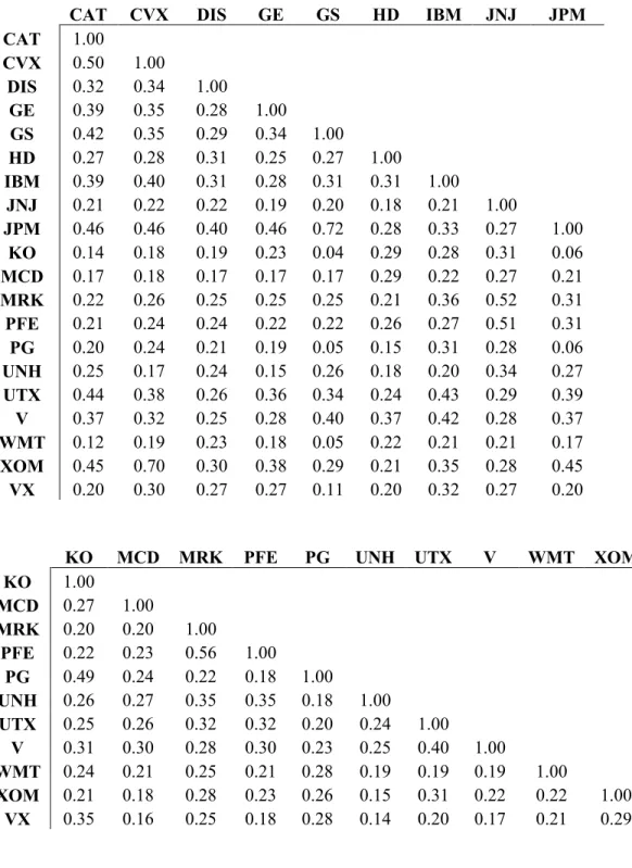
Table II.2: Correlation of Daily Returns in Estimation Period
- CAT CVX DIS GE GS HD IBM JNJ JPM
CAT 1.00
CVX 0.50 1.00
DIS 0.32 0.34 1.00
GE 0.39 0.35 0.28 1.00
GS 0.42 0.35 0.29 0.34 1.00
HD 0.27 0.28 0.31 0.25 0.27 1.00
IBM 0.39 0.40 0.31 0.28 0.31 0.31 1.00
JNJ 0.21 0.22 0.22 0.19 0.20 0.18 0.21 1.00
JPM 0.46 0.46 0.40 0.46 0.72 0.28 0.33 0.27 1.00
KO 0.14 0.18 0.19 0.23 0.04 0.29 0.28 0.31 0.06
MCD 0.17 0.18 0.17 0.17 0.17 0.29 0.22 0.27 0.21
MRK 0.22 0.26 0.25 0.25 0.25 0.21 0.36 0.52 0.31
PFE 0.21 0.24 0.24 0.22 0.22 0.26 0.27 0.51 0.31
PG 0.20 0.24 0.21 0.19 0.05 0.15 0.31 0.28 0.06
UNH 0.25 0.17 0.24 0.15 0.26 0.18 0.20 0.34 0.27
UTX 0.44 0.38 0.26 0.36 0.34 0.24 0.43 0.29 0.39
V 0.37 0.32 0.25 0.28 0.40 0.37 0.42 0.28 0.37
WMT 0.12 0.19 0.23 0.18 0.05 0.22 0.21 0.21 0.17
XOM 0.45 0.70 0.30 0.38 0.29 0.21 0.35 0.28 0.45
VX 0.20 0.30 0.27 0.27 0.11 0.20 0.32 0.27 0.20
KO MCD MRK PFE PG UNH UTX V WMT XOM
KO 1.00
MCD 0.27 1.00
MRK 0.20 0.20 1.00
PFE 0.22 0.23 0.56 1.00
PG 0.49 0.24 0.22 0.18 1.00
UNH 0.26 0.27 0.35 0.35 0.18 1.00
UTX 0.25 0.26 0.32 0.32 0.20 0.24 1.00
V 0.31 0.30 0.28 0.30 0.23 0.25 0.40 1.00
WMT 0.24 0.21 0.25 0.21 0.28 0.19 0.19 0.19 1.00
XOM 0.21 0.18 0.28 0.23 0.26 0.15 0.31 0.22 0.22 1.00
All of the assets are positively correlated over this period, with the average correlation 0.27. It is logical that all of the assets are positively correlated as they are all large-cap, US based companies.2
A point of note is the difference in the trend of returns during the estimation period and the forecast period. During the estimation period, the overall market was performed extremely well, with the Dow 30 growing 13.42% and 25.08% in 2016 and 2017 respectively; however, over the forecast period, the Dow 30 fell 5.63%. This discrepancy might lead to forecasted conditional variances and covariance matrices that don’t fit the return data in the forecast period well even though the estimated parameters fit the in-sample data well.
In order to maximize the frequency of data used without inducing a concerning amount of microstructure noise into the data, five minute data will be used to calculate intraday returns. However, in order to use all of the data possible, five minute returns will be taken five times every five minutes and then averaged for each day, meaning five minute ticks will be taken at minutes 1,6,11,16,…, and then another group taken at minutes 2,7,12,17,…, continuing on until
the fifth group is taken at minutes 5,10,15,20,…, etc. The five estimates of returns are then averaged together. This should smooth out any random extreme price discrepancies. This is simply a method to use all of the data provided at 1-minute intervals without introducing the microstructure noise that is inherent in 1-minute data.
IV.
Method
This section has the goal of outlining the theoretical backing and empirical models used in this research. First, the following is the basic notation used throughout the rest of the paper:
Let 𝑝𝑖,𝑡,𝑛 be the 𝑛th price of asset i on day t, and let 𝑟
𝑖,𝑡,𝑛 be the log 5-minute return at on day t at time n.
𝑟𝑖,𝑡,𝑛 = ln(𝑝𝑖,𝑡,𝑛) − ln(𝑝𝑖,𝑡,𝑛−5) (4.1)
Let 𝑅𝑡 be a matrix (i x n)of the returns for time t with n returns for all i assets.
𝑅𝑡 = [
𝑟1,𝑡,1 ⋯ 𝑟1,𝑡,𝑛
⋮ ⋱ ⋮
𝑟𝑖,𝑡,1 ⋯ 𝑟𝑖,𝑡,𝑛] (4.2)
Let 𝑅𝐶𝑣𝑡 be the realized covariance matrix on day t, and let 𝑅𝐶𝑡 be a realized correlation matrix on day t, with 𝛫𝑡 as a matrix with the realized variances, which is the sum of squared intraday returns, on the diagonal and zeros on all of the off-diagonal elements. Additionally, let a superscript T of a matrix represent the transpose of said matrix.
𝑅𝐶𝑣𝑡= 𝑅𝑖,𝑡∗ 𝑅𝑖,𝑡𝑇 (4.3)
𝑅𝐶𝑡 = 𝛫𝑡−1∗ 𝑅𝐶𝑣
𝑡∗ 𝛫𝑡−1 (4.4)
Let 𝑦𝑖,𝑡 be the demeaned daily return of asset i of day t, let 𝑦̅𝑖 be the average daily return of asset
i, and let 𝑦𝑡 be a vector of demeaned daily returns at time t for all assets i.
𝑦𝑖,𝑡 = ln(𝑝𝑖,𝑡,𝑐𝑙𝑜𝑠𝑒) − ln(𝑝𝑖,𝑡,𝑜𝑝𝑒𝑛) − 𝑦̅ (4.5) 𝑖
𝑦𝑡 = [ 𝑟𝑖,𝑡
⋮
i.
Exponential GARCH
The first step in forecasting conditional covariance with a DCC-GARCH model is estimating conditional variances for each asset individually, which can be accomplished through a univariate GARCH model or one of the many variations on a univariate GARCH. In this research, I will be estimating the conditional variances for each asset through an EGARCH model. This model has many advantages over a traditional GARCH model, as discussed in the literature review, but it also does not guarantee the model is stationary, so there may be no estimated unconditional variance. Therefore, in addition to an EGARCH model, I will also estimate the conditional variances with an EGARCH model that includes measures of realized variance as a signal. The in-sample fit and out of sample accuracy will be measured and the model that is shown to better estimate the conditional variance will be used to forecast the DCC models.
Consider the following model for demeaned returns. Let ℎ𝑖,𝑡 be the conditional variance for asset i on day t, and let 𝑧𝑖,𝑡 be defined as returns which are independent and identically distributed (i.i.d.) with an expected value of 0 and a variance of 1.
𝑦𝑖,𝑡 = √ℎ𝑖,𝑡∗ 𝑧𝑖,𝑡 (4.7)
Now consider the following specification of the EGARCH model:
log (ℎ𝑖,𝑡) = 𝜔 + 𝛽 log(ℎ𝑖,𝑡−1) + 𝜏1𝑧𝑖,𝑡−1+ 𝜏2(𝑧𝑖,𝑡−12− 1) (4.8)
Also, consider the Real-EGARCH model as specified by Hansen et. al, which is made up of a return equation similar to the traditional EGARCH model and a measurement equation that estimates a realized volatility measure. Let 𝑢𝑖,𝑡 represent the conditional variance signal derived from the realized volatility measure, and let 𝑥𝑖,𝑡 be the actual estimated realized volatility measure:
log (ℎ𝑖,𝑡) = 𝜔 + 𝛽 log(ℎ𝑖,𝑡−1) + 𝜏1𝑧𝑖,𝑡−1+ 𝜏2(𝑧𝑖,𝑡−12 − 1) + 𝜃𝑢𝑖,𝑡−1 (4.9)
log (𝑥𝑖,𝑡) = 𝜀 + 𝜑 log(ℎ𝑖,𝑡) + 𝛿1𝑧𝑖,𝑡+ 𝛿2(𝑧𝑖,𝑡2 − 1) + 𝑢
𝑖,𝑡 (4.10)
Similar to above, these parameters will be estimated by maximizing a quasi-log-likelihood as specified by Hansen et. al (Hansen et. al, 2012). It is important to note that, directly, the log-likelihood estimates of the EGARCH and Real-EGARCH models cannot be directly compared, as the Real-EGARCH includes the measurement equation, which results in a differently
structured quasi-log-likelihood function to maximize. However, the Real-EGARCH assumes independence between 𝑢𝑖,𝑡 and 𝑥𝑖,𝑡, which allows for the quasi log-likelihood function to be split up. One of the partial log-likelihood functions is equivalent to the log-likelihood function of the EGARCH model. These are the log-likelihoods that are compared.
Both of these estimations will two different estimates of the conditional variance for each asset which will be used to studentize returns, as specified in (4.7). These models will be
compared using the value of the maximized log-likelihood value of each asset for both models.
ii.
Constant Conditional Correlation
is assumed to be constant over the estimation and forecast period. Although this may not be a realistic assumption, it is important to include this measure in the comparison. Let 𝐶̅ be defined as follows:
𝐶̅ =1
𝑇∑ 𝑧𝑡−1∗ 𝑧𝑡−1 𝑇 𝑇
𝑡=1 (4.11)
Since this model requires no parameter estimation, the constant conditional correlation can be placed directly into log-likelihood measure that will be used to measure forecast accuracy along with the other estimated conditional covariance matrices from the DCC-GARCH models. It is important to note that CCC is nested inside of DCC-GARCH; therefore, DCC-GARCH should necessarily result in a higher in-sample log-likelihood value than the CCC model.
iii.
DCC-GARCH
The goal of the DCC-GARCH model is to model the conditional covariance of asset returns by estimating the variances and covariances separately. After modeling the conditional variances through a univariate GARCH process, the covariances are estimated through a
parameterized correlation matrix that ensures the modeled covariance matrix is positive definite. The parametrized correlation is modeled as a combination of the unconditional correlation between asset returns, the previous periods’ conditional parameterized correlation, and some
signal of previous periods’ returns. This research will alter the DCC model by changing the last
Similar to EGARCH model, the first step is to model the studentized returns. Let 𝐻𝑡 be the conditional covariance matrix at day t, and let 𝐻𝑡 be the conditional covariance matrix at time
t.
𝑦𝑡 = 𝐻𝑡1/2∗ 𝑧𝑡 (4.12)
This is a similar characterization as above in the EGARCH model, but it is in matrix form, considering returns of all assets in one model. Again, 𝑧𝑡 is i.i.d., the expected value is 0, and E[𝑧𝑡𝑧𝑡𝑇] = 𝐼. The conditional variances were estimated in the EGARCH models, and the
conditional covariance will now be estimated by estimating a parameterization of the correlation matrix, where 𝐶𝑡 is the correlation matrix at time t. Let 𝐷𝑡 be a matrix of the conditional standard deviations, with the conditional standard deviations on the diagonal and zeros on the
off-diagonals
𝐻𝑡= 𝐷𝑡∗ 𝐶𝑡∗ 𝐷𝑡 (4.13)
In order to obtain a positive definite correlation matrix during estimation of parameters and throughout the forecasting process, let 𝐶𝑡 be parameterized in the following way:
𝐶𝑡 = 𝐹𝑡−1∗ 𝑄𝑡∗ 𝐹𝑡∗−1 (4.14)
Let the parameters a and b be an estimated scalar where a and b are both positive and a + b < 1. 𝑧𝑡−1∗ 𝑧𝑡−1𝑇 acts as a low-frequency signal for future conditional variances.
𝑄𝑡 = (1 − 𝑎 − 𝑏)𝑄̅ + 𝑎(𝑧𝑡−1∗ 𝑧𝑡−1𝑇) + 𝑏 ∗ 𝑄𝑡−1 (4.15)
𝑄̅ =1
𝑇∑ 𝑧𝑡−1∗ 𝑧𝑡−1 𝑇 𝑇
𝑡=1 (4.16)
Additionally, let 𝐹𝑡∗ be specified as below. Let 𝑞
𝐹𝑡∗ = [
√𝑞1,1 … 0
⋮ ⋱ ⋮
0 … √𝑞20,20
] (4.17)
This type of parameterization forces that 𝐶𝑡 is positive definite, where the diagonals are
identically 1 and each element of the matrix must be bounded by [-1,1]. This model will simply be called DCC-GARCH.
The following is a model is an alteration of the DCC-GARCH model, replacing the previous signal with realized correlation, which uses intraday data as specified in (4.4). This model will be called RC-DCC:
𝑄𝑡𝑅𝐶 = (1 − 𝑎 − 𝑏)𝑄̅ + 𝑎𝑅𝐶𝑡−1+ 𝑏𝑄𝑡−1𝑅𝐶 (4.18)
Both the DCC-GARCH and the RC-DCC models’ parameters are estimated by maximizing the following function for T days in the estimation period:
ℒ = −1
2∑ log(𝑑𝑒𝑡(𝐶𝑡)) + 𝑧𝑡−1 𝑇∗ 𝐶
𝑡−1∗ 𝑧𝑡−1 𝑇
𝑡=1 (4.19)
This likelihood function assumes that asset returns are best described by the normal distribution.
iv.
Generalized Fisher Z-Transformation
The GFT is a log-transformation of a sample correlation matrix that increases the normality of the correlation estimates. This paper gives a brief overview of Archakov and Hansen’s proposed GFT, but the full explanation and derivation can be reviewed in their paper. The
Z-Transformation is a method to transform Pearson’s correlation coefficient so that it is normally
𝑧 =1 2log (
1+𝜌
1−𝜌) (4.20)
G = [
1 1
2ln ( 1+𝜌2,1
1−𝜌2,1)
1 2ln (
1+𝜌1,2
1−𝜌1,2) 1
] (4.21)
The above is the natural Fisher Z-transformation of a correlation matrix between two assets. There is research surrounding an element-wise Fisher Z-Transformation for an n x n matrix, meaning each off-diagonal element is transformed according to (4.20). However, this approach does not fulfill desirable requirements for a parameterization that the GFT fulfills (Archakov and Hansen 2018).
If A is a 2x2 matrix, then if G = logm(A):
G = [ 1
2ln (1 − 𝜌
2) 1
2ln ( 1+𝜌 1−𝜌) 1
2ln ( 1+𝜌 1−𝜌)
1
2ln (1 − 𝜌
2)] (4.22)
It follows that the off-diagonal elements are individually transformed identically to (4.21). To clarify, logm(A) is the logarithm of a matrix, which is not the same as taking the element-by-element log of a matrix. Archakov and Hansen’s paper argues that a generalized Fisher
Z-transformation is given by the logarithm of a correlation matrix of any dimension.
To give a general definition of the GFT: let B be an (n x m) matrix of demeaned returns, with m individual assets and n observations. Then let 𝐻𝑡 be the sample covariance matrix of 𝑋𝑖,𝑡, as defined previously.
𝐶𝑡 = [
1 ⋯ ∎
⋮ ⋱ ⋮
𝜎𝑚,1
𝜎𝑚2𝜎12 ⋯ 1
] = [
1 ⋯ ∎
⋮ ⋱ ⋮
𝜌𝑚,1 ⋯ 1
] (4.23)
The transformation of the correlation matrix is centered on the log transformation of the correlation matrix. The finalized GFT = γ(C) = offdiag(log(C)), where offdiag is a function that
stacks the off diagonal elements in the lower triangle of the matrix log(C) into a vector, and log(C) is the log function applied to the matrix C. If C is a symmetric positive definite matrix, which is assumed for all of our correlation matrices, with the below eigendecomposition. Let 𝑄𝑡 be an orthonormal matrix such that 𝑄𝑡𝑄𝑡𝑇 = 𝐼, and 𝛬𝑡 is a matrix with eigenvalues of C𝑡 on the diagonal and zeroes on all of the off-diagonal elements.
C𝑡= 𝑄𝑡𝛬𝑡𝑄𝑡𝑇 (4.24)
logm(C𝑡), then takes the following form. Let log(𝛬𝑡) be a matrix with the log of each eigenvalue of C𝑡 is on the diagonal and the off-diagonal elements are all zero.
logm (C𝑡) = 𝑄𝑡log(𝛬𝑡)𝑄𝑡𝑇 (4.25)
The finalized γ(C𝑡) is offdiag(logm(C𝑡)), which is a vector of the off-diagonals of log(C𝑡). To clarify the offdiag() function, below is an example:
R = [
𝑟11 𝑟12 𝑟13 𝑟21 𝑟22 𝑟23 𝑟31 𝑟32 𝑟33
] (4.26)
offdiag(R) = [ 𝑟21 𝑟31
𝑟32] (4.27)
In their paper, Archakov and Hansen show that there is an isomorphism between the set of n x n non-singular correlation matrices and ℝ𝑛(𝑛−1)2 and they also provide an iterative program
for the inverse mapping.
v.
James Stein Shrinkage
James Stein shrinkage can be applied to the GFT transformed vector of off-diagonal correlation elements γ(C𝑡) at the end of day t. The goal of this shrinkage is to decrease the magnitude of extreme estimates that are likely due to estimation error and parameter miss-estimation. The shrinkage of γ(C𝑡) will take the following form. Let 𝛾̅ be a vector of the average transformed correlation of each element over the estimation period, let γ(C𝑡) 𝑆 indicate the shrunk γ(C𝑡) at time t, and let s be a vector of shrinkage intensities indicates the shrinkage intensity.
γ(C𝑡) 𝑆 = 𝛾̅ + 𝑠(γ(C
𝑡) − 𝛾̅) (4.28)
This means the transformation correlation estimates will be shrunk towards the mean correlation of all of the assets at time t. It is important to note that the reasoning for 𝛾̅𝑡 being the shrinkage target. It is likely that the majority of these assets are positively correlated, so the accurate correlation of two assets is likely above zero, so if the shrinkage target is at zero, transformed correlation estimates could be shrunk away from the true value. Now, consider s, the shrinkage intensity, which will be calculated as follows. Let i be the number of assets, and let 𝜎𝑖2 be the variance of the correlation of each pair of assets over the estimation period. The smaller the 𝑠𝑖, the further the estimate is shrunk closer to the shrinkage target.
𝑠𝑖 = 1 − [
(𝑖−3) ∑ (𝑖
𝑗γ(C𝑡)𝑖− 𝛾̅)2𝜎𝑖
𝑠 = [ 𝑠1
⋮
𝑠𝑛] (4.30)
Additionally, consider a double-shrunk estimator, which is simply altering (4.27) in the following way:
γ(C𝑡) 𝑆_2 = 𝛾̅ +𝑆
2[γ(C𝑡) − 𝛾̅] (4.31)
This model simply shrinks the transformed correlation matrix farther towards the desired shrinkage target. This could be desired if the realized correlation matrix is expected to show extreme values. For example, if returns are extremely volatile, applying double shrinkage can possibly increase the explanatory power of the transformed realized correlation as a signal, removing the extreme values that could throw the estimation off and result in a poor fit and inaccurate forecast.
vi.
GFT-DCC
The following specification is essentially the same model as the RC-DCC with signal of shrunk realized correlation.
The following is the specification of the GFT-DCC model. Let 𝛾̅ be defined as above and let 𝛾−1(𝑥) be the inverse mapping from ℝ𝑛(𝑛−1)2 to the space of (n x n) non-singular correlation matrices. For clarification, 𝛫𝑡 is the signal that will be constructed by applying the GFT to a realized correlation matrix, applying shrinkage to the transformed correlation matrix, and then mapping the shrunk transformed matrix back into ℝ𝑛(𝑛−1)2 space.
𝛫𝑡 = 𝛾−1(γ(C𝑡) 𝑆) (4.33)
These parameters will be estimated with the same log-likelihood function as above. Lastly, consider the previous model with a double-shrunk transformed realized correlation matrices as defined in (4.30) with name GFT-DCC-2:
𝑄𝑡𝐺𝐹𝑇 = (1 − 𝑎 − 𝑏)𝑄̅ + 𝑎𝛹𝑡−1+ 𝑏𝑄𝑡−1𝐺𝐹𝑇 (4.34)
𝛹𝑡 = 𝛾−1(γ(C𝑡) 𝑆_2) (4.35)
This model is included because the shrinkage intensities calculated for this dataset, as defined in (4.28), are relatively high, meaning any extreme values that are desired to be shrunk towards the shrinkage target are not moved far out of extremity. The average shrinkage intensity is 0.8369, which may not shrink the data enough to avoid extreme values that taint the estimation. The comparison of the performance of a model with
Similar to above, these parameters will be estimated by maximizing (4.19).
vii.
Log-Likelihood
EGARCH models and a comparison between all of the different DCC models when the true conditional variance and covariance matrices are unknown.
The likelihoods of each model will be compared through some criterion such as the Akaike information criterion (AIC), which gives an estimate of the relative quality of statistical models for each set of data given the likelihood of each function and the number of parameters estimated. The model with the lowest AIC value is suggested to be the best fit model. The AIC values from each model can then be compared to interpret the probability that a model minimizes the relative information loss from the true data generating process when compared to the
supposed dominant model.
Let AIC𝑖 be the estimated AIC value of asset i, let p be the number of parameters estimated, and let ℒ𝑖 be the maximized log-likelihood for model j.
AIC𝑖 = 2 ∗ 𝑝 − 2 ∗ ℒ𝑖 (4.36)
Then the AIC values can be compared to find the relative goodness of fits of two models as specified below. Let i_low represent the model that has the minimum AIC𝑖, let 𝜔𝑖 be the relative probability that model i minimizes information loss when compared to model i_low.
𝜔𝑖 = exp (ℒ𝑖_𝑙𝑜𝑤− ℒ𝑖
2 ) (4.37)
For example, if 𝜔𝐷𝐶𝐶−𝐺𝐴𝑅𝐶𝐻 = .005 and it is being compared to GFT-DCC, then DCC-GARCH is .005 times more likely to minimize information loss of the true data generating model than GFT-DCC.
model, then the AIC is necessarily going to suggest that the model with the higher log-likelihood is the dominant model. Therefore, it is not necessary to compute the AIC values to find the model with best fit and forecasting value. However, computing the AIC values allows for a direct way to compare the power of each model through (4.37).
viii.
Mean-Variance Optimization
A second method to test the accuracy of the forecast is to optimize a portfolio based off of the forecasted conditional variances based on some certain criteria. For this research, the obvious choice is global mean-variance portfolio optimization, which minimizes portfolio return variance, independent of asset returns. This method allows for a truly out-of-sample test of the forecasted covariance without having to also include forecasted returns in the estimation of weights, which would not be desirable as then the performance of the portfolio would depend jointly on the forecasted returns and the forecasted variance.
Consider the following specifications of the optimization model. Let 𝑟𝑡𝑝 be the return of the portfolio at time t, let 𝑝𝑖,𝑡 be the open-to-close return of asset i at time t, let 𝑃𝑡 simply be a 20x1 vector of stacked daily returns for each asset, and let 𝑤𝑡 be a 1x20 vector of portfolio weights at time t.
𝑝𝑖,𝑡 = ln(𝑝𝑖,𝑡,𝑐𝑙𝑜𝑠𝑒) − ln(𝑝𝑖,𝑡,𝑜𝑝𝑒𝑛) (4.38)
𝑃𝑡 = ⌈ 𝑝1,𝑡
⋮
𝑝20,𝑡⌉ (4.39)
The portfolio weights is what are being optimized to minimize portfolio variance, which is defined as follows. Let 𝜎𝑃2 be the portfolio variance and let 𝐻
𝑡 be the conditional covariance matrix at time t as defined previously.
𝜎𝑃2 = 𝑤𝑡∗ 𝐻𝑡∗ 𝑤𝑡 (4.41)
Certain restrictions are placed on 𝑤𝑡, specifically that the weights must sum to one, and each must weight is bounded by [-1,1].
A weight vector will be estimated for each day for each of the six DCC models, and whichever model estimates weights that allow for the lowest variance in portfolio returns over the forecast period is considered the model with the best forecast. The higher the variance of portfolio returns over the forecast period, the less accurate the forecasted variance.
V.
Results
i.
EGARCH and Real-EGARCH Models
In this section, I present the results of the EGARCH and Real-EARCH models, discuss the estimated coefficients, and compare the in-sample and out-of-sample log-likelihoods for each asset.
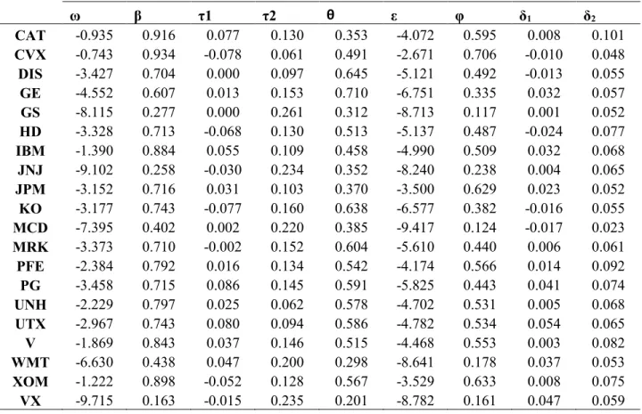
Referencing Table V.1, it is important to note that almost all of these coefficients are significant, with the insignificant coefficients largely being made up by the intercept estimates ω
and ε. Since the goal of this research is not to evaluate the difference between EGARCH and
Table V.1: Coefficients of Real-EGARCH Model3
ω β τ1 τ2 θ ε φ δ1 δ2
CAT -0.935 0.916 0.077 0.130 0.353 -4.072 0.595 0.008 0.101
CVX -0.743 0.934 -0.078 0.061 0.491 -2.671 0.706 -0.010 0.048
DIS -3.427 0.704 0.000 0.097 0.645 -5.121 0.492 -0.013 0.055
GE -4.552 0.607 0.013 0.153 0.710 -6.751 0.335 0.032 0.057
GS -8.115 0.277 0.000 0.261 0.312 -8.713 0.117 0.001 0.052
HD -3.328 0.713 -0.068 0.130 0.513 -5.137 0.487 -0.024 0.077
IBM -1.390 0.884 0.055 0.109 0.458 -4.990 0.509 0.032 0.068
JNJ -9.102 0.258 -0.030 0.234 0.352 -8.240 0.238 0.004 0.065
JPM -3.152 0.716 0.031 0.103 0.370 -3.500 0.629 0.023 0.052
KO -3.177 0.743 -0.077 0.160 0.638 -6.577 0.382 -0.016 0.055
MCD -7.395 0.402 0.002 0.220 0.385 -9.417 0.124 -0.017 0.023
MRK -3.373 0.710 -0.002 0.152 0.604 -5.610 0.440 0.006 0.061
PFE -2.384 0.792 0.016 0.134 0.542 -4.174 0.566 0.014 0.092
PG -3.458 0.715 0.086 0.145 0.591 -5.825 0.443 0.041 0.074
UNH -2.229 0.797 0.025 0.062 0.578 -4.702 0.531 0.005 0.068
UTX -2.967 0.743 0.080 0.094 0.586 -4.782 0.534 0.054 0.065
V -1.869 0.843 0.037 0.146 0.515 -4.468 0.553 0.003 0.082
WMT -6.630 0.438 0.047 0.200 0.298 -8.641 0.178 0.037 0.053
XOM -1.222 0.898 -0.052 0.128 0.567 -3.529 0.633 0.008 0.075
VX -9.715 0.163 -0.015 0.235 0.201 -8.782 0.161 0.047 0.059
All of the coefficients are positive and significant, suggesting that there is a substantial
relationship between lagged realized variance and conditional variance. Additionally, between EGARCH4 and Real-EGARCH, the β coefficient’s magnitude dropped by a non-insignificant
amount without a large change in the standard errors, suggesting that the β coefficient loses some
explanatory power when including a measure of realized variance.
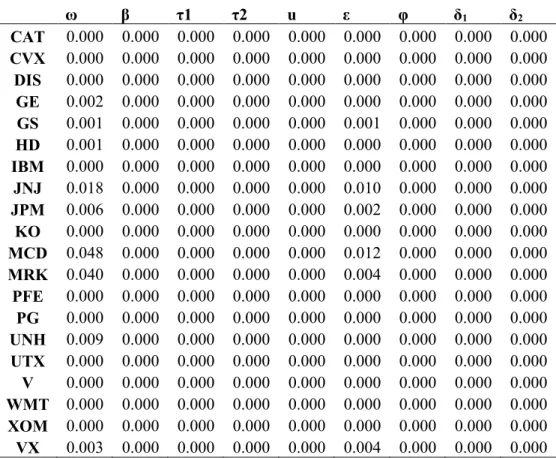
3 A table of robust standard errors are available in the appendix (V.2)
4A table of coefficients of the EGARCH model and a table of robust standard errors of these coefficients are
Table V.5: Average Log-Likelihood of EGARCH and Real-EGARCH
In-Sample Out-of-Sample
EGARCH 1771.36 -3095.91
Real-EGARCH 1883.32 664.63
Table V.5 gives further credence to Real-EGARCH outperforming EGARCH both in-sample and out-of-in-sample.5 During the estimation period, Real-EGARCH outperforms EGARCH
for every asset. During the forecast period, there are assets where Real-EGARCH outperforms EGARCH and visa-versa. The discrepancy in the average out-of-sample log-likelihood can be blamed on a small number of assets displaying extremely negative log-likelihood values. This is likely due to the EGARCH model’s inability to ensure the existence of an unconditional
variance. As the EGARCH process moves further into the forecast period, the forecasted conditional variance converges to the unconditional variance; however, if the unconditional variance does not exist, the forecasted variances may display extreme behavior. Due to this, the forecasted conditional covariance matrices will only be estimated using conditional variances estimated from the Real-EGARCH model. The in-sample models will be estimated with conditional variances estimated from both EGARCH and Real-EGARCH models, but the forecasted covariance matrices will only use Real-EGARCH forecasted conditional variances.
ii.
DCC-GARCH Models
In this section, I will present the estimated coefficients of the DCC models, including the GFT-DCC variations, and discuss the in-sample and out-of-sample log-likelihood comparisons.
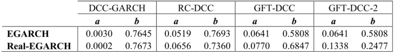
Table V.7 displays the estimated coefficients for the DCC models laid out in the model section. Two estimated coefficients are shown for each coefficient of each DCC model, the first being the estimated coefficient from a model using the conditional variances derived from the EGARCH model and the second being the estimated coefficient from a model using the conditional variances derived from the Real-EGARCH model.
Table V.7: DCC Model Coefficient Estimates
DCC-GARCH RC-DCC GFT-DCC GFT-DCC-2
a b a b a b a b
EGARCH 0.0030 0.7645 0.0519 0.7693 0.0641 0.5808 0.0641 0.5808
Real-EGARCH 0.0002 0.7673 0.0656 0.7360 0.0770 0.6847 0.1338 0.2477
The first point of note is that the b coefficients in the last three models with EGARCH conditional variance specification are all essentially 0, suggesting that the GFT realized
correlation has little impact on forecasting conditional covariance matrices. However, this does not hold when comparing the b coefficients in the Real-EGARCH specified GFT models. This gives more credence to using only the Real-EGARCH model in the forecast for conditional variances and covariance matrices.
Also, it is important to note the jump in the magnitude of the bcoefficient when
Table V.8: In-Sample and Out-of-Sample Log-Likelihood of DCC Models
In-Sample Out-of-Sample
EGARCH Real-GARCH Real-GARCH
CCC -3719.16 -3628.08 -9053.88
DCC-GARCH -3310.52 -3212.16 -3737.34
RC-DCC -3292.38 -3189.26 -3649.69
GFT-DCC -3292.93 -3189.27 -3654.77
GFT-DCC-S -3299.97 -3194.35 -3673.68
The above table suggests that RC-DCC is the dominant model in both the in-sample and out-of-sample fit. Therefore, when computing the ω for each model according to (4.35), ℒ𝑗_𝑙𝑜𝑤 is equivalent to ℒ𝑅𝐶−𝐷𝐶𝐶.
Table V.9: Ratio that Model Induces Minimum Information Loss in Comparison to RC-DCC
In-Sample Out-of-Sample
EGARCH Real-GARCH Real-GARCH
𝜔𝐶𝐶𝐶 4.4581E-186 2.6419E-191 0
𝜔𝐷𝐶𝐶−𝐺𝐴𝑅𝐶𝐻 1.32185E-08 1.13139E-10 8.57916E-39
𝜔𝑅𝐶−𝐷𝐶𝐶 1 1 1
𝜔𝐺𝐹𝑇−𝐷𝐶𝐶 0.576315769 0.995347876 0.006226314
𝜔𝐺𝐹𝑇−𝐷𝐶𝐶−2 0.000502194 0.006157251 3.816E-11
The GFT-DCC models outperformed the DCC-GARCH model under both specifications for conditional variance.6 Lastly, the CCC model was included simply as a check to make sure
the models were seemingly correctly specified. The CCC model is nested inside of a DCC model, and therefore a DCC model should outperform, or at least perform exactly as well, as the CCC model. This holds for the in-sample estimation.
When comparing log-likelihoods of the models in the out-of-sample data, the expected results are similarly met. Both of the GFT models were dominant to the DCC-GARCH but far more inferior to the RC-DCC model than it was in the in-sample estimation. This suggests that the GFT transformed signal, in this instance being realized correlation, acts as a worse signal than the untransformed signal.
Additionally, GFT-DCC performed better than GFT-DCC-S, suggesting bringing extreme values towards a more realistic value decreased the forecasting accuracy. This might be due to the condition of the market in the forecast period. The estimation period was a period of relatively low volatility and high returns, while the forecast period experienced a much larger amount of volatility in returns. Decreasing extreme values in the signal might have been
beneficial for the estimation period, but the extreme values in the realized correlation during the forecast period may have actually been realistic and shrinking this data removed valuable information from the market. Removing the extreme values would also increase the time estimated variance require to catch up following a shock.
Overall, the RC-DCC was the dominant model considering the log-likelihood of the model at the estimated parameters and the AIC values. The GFT models outperformed the
traditional DCC-GARCH model in both the in-sample and out-of-sample periods. However, the GFT models performed significantly worse in the out-of-sample estimation period when
compared to the dominant RC-DCC model. This may be due to the nature of the returns during the forecast period.
iii.
Mean-Variance Optimization
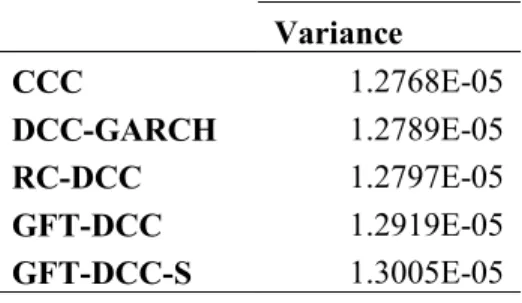
This section reviews the results of the mean-variance portfolio optimization that took the forecasted covariance matrices as inputs. The weights were re-estimated daily in the forecast period with the goal of minimizing portfolio variance. The model that yields weights for each asset that result in the lowest variance in daily returns over the forecast period is the model considered to give the best, most useful, forecasted variances over the entire period.
Table V.11: Variance of Portfolio Returns over Forecast Period by Model
Variance
CCC 1.2768E-05
DCC-GARCH 1.2789E-05
RC-DCC 1.2797E-05
GFT-DCC 1.2919E-05
GFT-DCC-S 1.3005E-05
suggesting that the GFT models may not perform as well out-of-sample as in-sample, and the GFT models may not be an improvement on the traditional DCC-GARCH.
It is important to note that these differences in variances are extremely small; these models track each other fairly closely in weights and result in extremely similar returns.
Therefore, while this is still a criterion to consider, the log-likelihood and AIC criteria might give a better intuition in determining the dominant model.
VI.
Conclusion
In this paper, I have evaluated the validity of including the Generalized Fisher
Z-Transformation into a covariance forecasting model, estimating if including the signal given by GFT transformed data in the model outperforms the traditional DCC-GARCH model and a DCC model with realized correlation included as a signal. The theoretical outcome is that both the RC-DCC and GFT-RC-DCC models will outperform the traditional RC-DCC-GARCH model in both in-sample model fit and out-of-in-sample forecast accuracy. This research also discussed the comparative value of a traditional EGARCH model and an EGARCH model that incorporates realized volatility in its estimation.
The results were as expected for the EGARCH models. The Real-EGARCH model outperformed the EGARCH model in both in-sample and out-of-sample evaluations, and the EGARCH model resulted in non-stationary results for some assets while the Real-EGARCH did not encounter this issue. Therefore, the DCC models used the conditional variances estimated through the Real-EGARCH for forecasting.
Similarly, the results were largely as expected when considering the in-sample estimation. The RC-DCC, which has empirical precedent to outperform DCC-GARCH, fit the in-sample data the best out of all five models soundly, with the GFT models also outperforming the
DCC-GARCH and CCC models. Additionally, as the shrinkage increased in the GFT model, the worse fit of the in-sample data. This suggests that the GFT is a good signal for measuring conditional covariance, improving upon DCC-GARCH and performing similarly to the RC-DCC model.
VVII. Appendix
Table II.3: Correlation of Daily Returns in Forecast Period
CAT CVX DIS GE GS HD IBM JNJ JPM
CAT 1.00
CVX 0.35 1.00
DIS 0.47 0.29 1.00
GE 0.27 0.26 0.21 1.00
GS 0.49 0.42 0.48 0.25 1.00
HD 0.44 0.24 0.48 0.16 0.48 1.00
IBM 0.43 0.26 0.47 0.39 0.46 0.46 1.00
JNJ 0.32 0.38 0.32 0.18 0.43 0.39 0.39 1.00
JPM 0.46 0.41 0.45 0.31 0.77 0.51 0.52 0.46 1.00
KO 0.27 0.27 0.32 0.12 0.29 0.39 0.24 0.50 0.29
MCD 0.29 0.15 0.29 0.23 0.28 0.37 0.24 0.51 0.33
MRK 0.38 0.33 0.37 0.22 0.43 0.37 0.39 0.61 0.35
PFE 0.30 0.37 0.39 0.15 0.43 0.42 0.38 0.64 0.40
PG 0.14 0.26 0.13 0.21 0.15 0.15 0.27 0.46 0.20
UNH 0.40 0.35 0.49 0.25 0.43 0.52 0.51 0.53 0.52
UTX 0.65 0.27 0.48 0.36 0.53 0.58 0.50 0.38 0.48
V 0.49 0.23 0.48 0.15 0.44 0.51 0.57 0.31 0.47
WMT 0.27 0.31 0.25 0.19 0.31 0.44 0.24 0.41 0.33
XOM 0.37 0.72 0.37 0.29 0.47 0.24 0.26 0.42 0.45
VX 0.09 0.23 0.27 0.17 0.13 0.25 0.19 0.45 0.20
KO MCD MRK PFE PG UNH UTX V WMT XOM
KO 1.00
MCD 0.46 1.00
MRK 0.37 0.35 1.00
PFE 0.49 0.30 0.68 1.00
PG 0.50 0.32 0.33 0.28 1.00
UNH 0.30 0.37 0.52 0.50 0.26 1.00
UTX 0.35 0.37 0.42 0.37 0.21 0.42 1.00
V 0.23 0.23 0.34 0.30 0.08 0.47 0.50 1.00
WMT 0.40 0.34 0.36 0.35 0.39 0.24 0.29 0.17 1.00
XOM 0.35 0.20 0.38 0.40 0.27 0.41 0.33 0.29 0.25 1.00
Table V.2: Robust Standard Errors of Real-EGARCH Coefficients
ω β τ1 τ2 u ε φ δ1 δ2
CAT 0.000 0.000 0.000 0.000 0.000 0.000 0.000 0.000 0.000
CVX 0.000 0.000 0.000 0.000 0.000 0.000 0.000 0.000 0.000
DIS 0.000 0.000 0.000 0.000 0.000 0.000 0.000 0.000 0.000
GE 0.002 0.000 0.000 0.000 0.000 0.000 0.000 0.000 0.000
GS 0.001 0.000 0.000 0.000 0.000 0.001 0.000 0.000 0.000
HD 0.001 0.000 0.000 0.000 0.000 0.000 0.000 0.000 0.000
IBM 0.000 0.000 0.000 0.000 0.000 0.000 0.000 0.000 0.000
JNJ 0.018 0.000 0.000 0.000 0.000 0.010 0.000 0.000 0.000
JPM 0.006 0.000 0.000 0.000 0.000 0.002 0.000 0.000 0.000
KO 0.000 0.000 0.000 0.000 0.000 0.000 0.000 0.000 0.000
MCD 0.048 0.000 0.000 0.000 0.000 0.012 0.000 0.000 0.000
MRK 0.040 0.000 0.000 0.000 0.000 0.004 0.000 0.000 0.000
PFE 0.000 0.000 0.000 0.000 0.000 0.000 0.000 0.000 0.000
PG 0.000 0.000 0.000 0.000 0.000 0.000 0.000 0.000 0.000
UNH 0.009 0.000 0.000 0.000 0.000 0.000 0.000 0.000 0.000
UTX 0.000 0.000 0.000 0.000 0.000 0.000 0.000 0.000 0.000
V 0.000 0.000 0.000 0.000 0.000 0.000 0.000 0.000 0.000
WMT 0.000 0.000 0.000 0.000 0.000 0.000 0.000 0.000 0.000
XOM 0.000 0.000 0.000 0.000 0.000 0.000 0.000 0.000 0.000
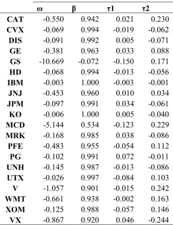
Table V.3: Coefficients of EGARCH Model
ω β τ1 τ2
CAT -0.550 0.942 0.021 0.230
CVX -0.069 0.994 -0.019 -0.062
DIS -0.091 0.992 0.005 -0.071
GE -0.381 0.963 0.033 0.088
GS -10.669 -0.072 -0.150 0.171
HD -0.068 0.994 -0.013 -0.056
IBM -0.003 1.000 -0.003 -0.001
JNJ -0.453 0.960 0.010 0.034
JPM -0.097 0.991 0.034 -0.061
KO -0.006 1.000 0.005 -0.040
MCD -5.144 0.534 -0.123 0.229
MRK -0.168 0.985 0.038 -0.086
PFE -0.483 0.955 -0.054 0.112
PG -0.102 0.991 0.072 -0.011
UNH -0.145 0.987 -0.013 -0.086
UTX -0.026 0.997 -0.084 0.103
V -1.057 0.901 -0.015 0.242
WMT -0.661 0.938 -0.002 0.163
XOM -0.125 0.988 -0.057 0.146
Table V.4 Robust Standard Error of EGARCH Coefficients
ω β τ1 τ2
CAT 0.149 0.015 0.002 0.002
CVX 0.000 0.000 0.000 0.000
DIS 0.000 0.005 0.008 0.000
GE 0.056 0.002 0.002 0.001
GS 4.587 0.016 0.009 0.048
HD 0.000 0.000 0.000 0.000
IBM 0.000 0.000 0.000 0.000
JNJ 1.362 0.061 0.041 0.011
JPM 0.000 0.000 0.000 0.000
KO 0.000 0.000 0.000 0.000
MCD 9.272 0.012 0.006 0.077
MRK 0.000 0.000 0.000 0.000
PFE 0.429 0.023 0.001 0.004
PG 0.001 0.002 0.001 0.000
UNH 0.000 0.001 0.000 0.000
UTX 0.027 0.002 0.001 0.000
V 4.254 0.101 0.004 0.038
WMT 0.157 0.008 0.000 0.001
XOM 0.015 0.006 0.003 0.000
Table V.6: Log-Likelihoods for EGARCH and Real-GARCH
In-Sample Out-of-Sample
EGARCH Real-EGARCH EGARCH Real-EGARCH
CAT 1519.39 1622.33 555.23 522.43
CVX 1719.27 1770.95 -12529.34 644.24
DIS 1797.83 1902.55 -4130.03 653.40
GE 1720.61 1872.14 603.35 606.36
GS 1609.75 1767.04 695.39 655.91
HD 1800.26 1891.25 -10539.67 688.16
IBM 1803.93 1907.16 461.13 694.65
JNJ 1911.76 2049.61 715.50 559.09
JPM 1711.60 1799.66 -4361.19 679.56
KO 1926.66 2030.14 -10615.01 774.41
MCD 1862.91 2029.29 698.39 552.00
MRK 1759.89 1869.51 -11797.57 675.86
PFE 1776.13 1862.46 713.54 692.88
PG 1877.42 2002.96 -45.24 712.41
UNH 1730.12 1798.92 -4578.17 704.16
UTX 1770.10 1893.09 710.95 704.47
V 1781.68 1894.31 725.60 706.00
WMT 1783.31 1921.28 730.70 683.49
XOM 1785.60 1881.28 738.00 700.28
VX 1778.97 1900.41 -10669.74 682.80
Table V.10: Ratio that Model Induces Minimum Information Loss in Comparison to GFT-DCC
In-Sample Out-of-Sample
EGARCH Real-GARCH Real-GARCH
𝜔𝐶𝐶𝐶 7.7356E-186 2.6543E-191 0
𝜔𝐷𝐶𝐶−𝐺𝐴𝑅𝐶𝐻 2.29363E-08 1.13668E-10 1.37789E-36
𝜔𝑅𝐶−𝐷𝐶𝐶 1.735159879 1.004673868 160.6086674
𝜔𝐺𝐹𝑇−𝐷𝐶𝐶 1 1 1
References
Andersen, T. G., Bollerslev, T., Diebold, F. X., & Labys, P. (2000). The Distribution of Realized Exchange Rate Volatility. Exchange Rate Economics, 96, 42-55.
doi:10.7551/mitpress/2897.003.0005
Bandi, F. M., & Russell, J. R. (2008). Microstructure Noise, Realized Variance, and Optimal Sampling. Review of Economic Studies, 75(2), 339-369.
doi:10.1111/j.1467-937x.2008.00474.x
Barndorff-Nielsen, O. E., & Shephard, N. (2002). Econometric analysis of realized volatility and its use in estimating stochastic volatility models. Journal of the Royal Statistical Society: Series B (Statistical Methodology), 64(2), 253-280. doi:10.1111/1467-9868.00336 Beenstock, M., & Chan, K. (2009). Economic Forces In The London Stock Market. Oxford
Bulletin of Economics and Statistics, 50(1), 27-39. doi:10.1111/j.1468-0084.1988.mp50001002.x
Caporin, M., & Mcaleer, M. (2011). Do We Really Need Both Bekk And Dcc? A Tale Of Two Multivariate Garch Models. Journal of Economic Surveys, 26(4), 736-751.
doi:10.1111/j.1467-6419.2011.00683.x
Corey, D. M., Dunlap, W. P., & Burke, M. J. (1998). Averaging Correlations: Expected Values and Bias in Combined Pearsons and FisherszTransformations. The Journal of General Psychology, 125(3), 245-261. doi:10.1080/00221309809595548
Engle, R. (1982) Autoregressive Conditional Heteroscedasticity with Estimates of the Variance of United Kingdom Inflation. Econometrica, 50, 987-1007. doi.org/10.2307/1912773 Engle, R. F. (1999). Dynamic Conditional Correlation - A Simple Class of Multivariate GARCH
Models. SSRN Electronic Journal. doi:10.2139/ssrn.236998
Engle, R. F., & Kroner, K. F. (1995). Multivariate Simultaneous Generalized ARCH. Econometric Theory, 11(01), 122. doi:10.1017/s0266466600009063
Fan, J., Fan, Y., & Lv, J. (2008). High dimensional covariance matrix estimation using a factor model. Journal of Econometrics, 147(1), 186-197. doi:10.1016/j.jeconom.2008.09.017 Hansen, P. R., Huang, Z., & Shek, H. H. (2010). Realized GARCH: A Joint Model of Returns
and Realized Measures of Volatility. SSRN Electronic Journal. doi:10.2139/ssrn.1533475 Huang, Y., Su, W., & Li, X. (2010). Comparison of BEKK GARCH and DCC GARCH Models:
An Empirical Study. Advanced Data Mining and Applications Lecture Notes in Computer Science, 99-110. doi:10.1007/978-3-642-17313-4_10
Kim, S. Y., & Lee, Y. H. (2006). Comparison of a Class of Nonlinear Time Series models (GARCH, IGARCH, EGARCH). Korean Journal of Applied Statistics, 19(1), 33-41. doi:10.5351/kjas.2006.19.1.033
Leonard, T., & Hsu, J. S. (1992). Bayesian Inference for a Covariance Matrix. The Annals of Statistics, 20(4), 1669-1696. doi:10.1214/aos/1176348885