VARIANCES OF LENGTH AND SURFACE AREA ESTIMATES BY SPATIAL GRIDS: PRELIMINARY STUDY

VARIANCES OF LENGTH AND SURFACE AREA ESTIMATES

BY SPATIAL GRIDS: PRELIMINARY STUDY

JI

ˇ

JAN

´

ˇ

LUCIE

KUB´

´

Institute of Physiology, Academy of Sciences of the Czech Republic, V´ıdeˇnsk´a 1083, CZ-142 20 Praha, Czech Republic

e-mail: [email protected], [email protected]

(Accepted December 4, 2009)

ABSTRACT

Periodic spatial grids can be used for unbiased estimation of length and surface area of objects by counting or measuring intersections of the objects with the grids. The estimators are theoretically based on discrete approximation of well established integral geometric formulas. The variance of the estimates depends on properties of both the grid and the measured objects. Main results of the theory of variance of the isotropic uniform random (IUR) volume estimation by spatial grids, especially a formula relating the variance of the volume estimator with the object surface area and the grid constant, are recapitulated. To identify main features of length and surface area IUR estimates the variance due to rotation and simple asymptotic formulas for the residual variance of estimates of selected model objects is calculated. Surface area estimates by multiple grids of parallel lines in 3D and of the variance of length estimates by periodic grids of planes or spheres in d-dimensional space are studied.

Keywords: stereology, variance, 3D.

INTRODUCTION

Basic geometrical characteristics of 2D or 3D objects can be estimated by counting or measuring intersections of the objects with randomized periodic patterns of manifolds (Barbier, 1860; Santal´o, 1976; Cruz-Orive, 1997). Estimation of geometrical characteristics by measuring the objects intersections with the randomized probes can be regarded as a generalization of the classical topic of stereology – estimation of the characteristics measuring lower dimensional randomized sections of the objects. The formulas for unbiased estimators using intersections with randomized spatial grids follow from well established general formulas of integral geometry (Baddeley and Vedel-Jensen, 2005). On the other hand the variance of the estimates may depend on properties of both the grid and the measured objects in a complicated way.

The variance of volume estimation by measuring intersection of the object with arbitrary periodic grid in random position is already well understood. A useful approximate formula (Eq. 1) for the variance using only simple characteristic of the measured object is available. The formula for variance ofd₋dimensional volume estimate by point lattice was proved in (Hlawka,1950) for strictly convex sets with 6d₋times differentiable support function, the proof for convex sets or sets withC1.5 smooth boundary can be found in (Jan´aˇcek,2008) and it can be easily generalized to an arbitrary periodic grid. The volume of a bounded

object K in d₋dimensional space can be estimated by a point counting method using regular point lattice T_=AZd_inRd_{, whereZis the set of integers andAis a} regular matrix. The number of points of the randomly shifted point lattice inside the object multiplied by the specific volume of the point is an unbiased estimate of the volume. Under mild regularity conditions on the object K the variance of the estimator with the randomly rotated lattice scaled by the factoru>0 is

CTHd−1(∂K)Φ ¡

u−1¢ud+1

(Jan´aˇcek,2008), whereCTis a constant of the lattice, Hd−1(∂K)is the surface measure of the object,Φ_≥0 is a function which ergodic average tends to 1:

lim x→+∞

1

x ˆ x

0

Φ(t)dt=1.

The constant of the lattice can be expressed as

CT= ¡

2π2_dκ

d ¢−1

∑ξ_ξ6=_∈T∗0 |ξ|−d−1 where T∗=A−1Zd and κd is the volume of the unit ball in Rd. The value of the coefficient is approximately 0.072 837 for the quadratic lattice and 0.071 701 for the hexagonal lattice normalized to unit intensity in plane, 0.066 649 for the cubic lattice, 0.064 350 for the normalized body centered cubic lattice and 0.064 390 for the normalized face centered cubic lattice in space.

The result can be easily generalized from the counting measure of lattice T _{to an arbitrary} T₋ periodic measureµwith constant of the measureCµ =

¡ 2π2_dκ

d ¢−1

∑ξ_ξ6=_∈T∗0 ¯

coefficients of the measure (Jan´aˇcek,2006). Software package pgs for calculation of coefficients of various grids is available (Kiˆeu and Mora,2006).

For the purpose of the variance estimation the function Φ oscillating around 1 is neglected and the variance can be expressed approximately:

Var_(estV)∼_=CSHd−1_(∂K)N−

d+1

d

V (1)

where NV =|A|−1 is the grid points intensity and the lattice S _{is the homothetic copy of the point lattice} T _{with unit intensity. Similar simple approximations} for estimators of length or surface area are not yet known. The aim of this paper is to study the behavior of variance of selected estimators of length or surface area, design of the expressions for the estimators variance similar to Eq.1and evaluation of the coefficients in the expressions.

The length of a fibre-like structure in Rd can be measured with a randomly rotated and shifted (IUR) periodic grid of surfaces. The surface area of objects inRd can be estimated by counting intersections with a grid of lines. The variances of the estimators can be decomposed into the variance due to the orientation of the grid and to the residual component of variance:

Var_{(estQ) =}

Var_g∈SO

d(E(estQ|g)) +Eg∈SOd(Var(estQ|g)),

whereQis either length (L) or surface area (S) andSOd is the group of rotations inRd.

The variances of length or surface area estimates in

Rdusing spatial grids due to orientation are calculated in the same way as the variance of the surface area estimators using combined projection, treated in the following section.

VARIANCE OF SURFACE AREA

ESTIMATE IN

_R

_{USING TOTAL}

PROJECTION

Crofton formula relates the suface area of a convex body to the mean area of its isotropic projection. Surface area of a convex body inRdis average area of its projection multiplied bydκd/κd−1 whereκd is the volume of the unit ball inRd and using this equality we can construct an estimator of the surface area from the object total projection area (area weighted by Euler characteristics of projection inverse, seeSerra,1982):

estS= dκd

κ_d−1Atot

Variance of the projection area depends on the object anisotropy, i.e., on the distribution of the angles between the normals to the body. It is well known that the variance of the surface area estimators can be decreased by using average of areas of projections into a set of directions (with fixed mutual position, e.g., perpendicular) instead of one direction. The decrease of the variance is due to a negative covariances of the projections areas (Mattfeldtet al.,1985).

The formula for coefficient of variation (CV) of surface estimator from multiple weighted projection areas of a body (Jan´aˇcek,1999) is:

CV2=

ˆ π₂

0 ˆ π₂

0

Kd(ψ,χ)dF(ψ)dG(χ) , (2)

whereF is the distribution function of angles between normals to the object surface, G is the distribution function of angles between projections directions and the kernelKdis defined as

Kd(ψ,χ) = õ

dκd 2κd−1

¶2ˆ

SOd

|(gy,x) (gu,v)_|dg₋1 !

.

Kd(ψ,χ) can be evaluated either by direct integration or using convolution formula and Parseval equality for harmonic analysis onSd−1. For details and

examples see Appendix A.

LENGTH ESTIMATION BY THE

GRID OF SURFACES

The length of a curve inRd can be estimated from the number of intersection of the curve with a spatial grid of planes

estL= dκd 2κd−1

N SV

,

whereN is the number of intersections and SV is the surface area of the grid per unit volume. The variance of the estimator of the length due to orientation can be calculated by Eq.2 substituting forF the distribution function of angles between the tangents to the curve and forGthe distribution function of angles between the normals to the grid surfaces. The simplest of grids of surfaces is the grid composed of parallel planes. The grids with different directions of normals can be combined obtaining decreased variance due to orientation. The variance is decreased due to negative covariances as in the case of surface estimation by projections. The residual component of variance, E_g∈SO

d(Var(estL|g)), is the mean over all orientations

of an integral of total projection of the space curve to a line of given orientation. The total projection of the space curve to a line is a step function and the variance of integral estimate of such step function is well known (Moran,1950). An approximation of the residual component of variance of estimate of lengthL

of the objectKcomposed of space curves by applying grids of parallel hyperplanes inRd then follows from differential geometry:

E_g∈SO

d(Var(estL|g))∼=C

L

GκABS(K)SV−2,

κABS_{(K) =}

ˆ

K|

κ_|ds+π 4

¡

Nends+Nodd branchings¢,

C_GL= 1 3π

µ

dκd 2κ_d−1

¶2

,

where SV is the grid surface intensity,κ is curvature of the curve (i.e., the reciprocal of the radius of the osculating circle), Nends is number of endings of curves, Nodd branchings is number of branchings where an odd number of curves is joining together andκd is the volume of the unit ball inRd.

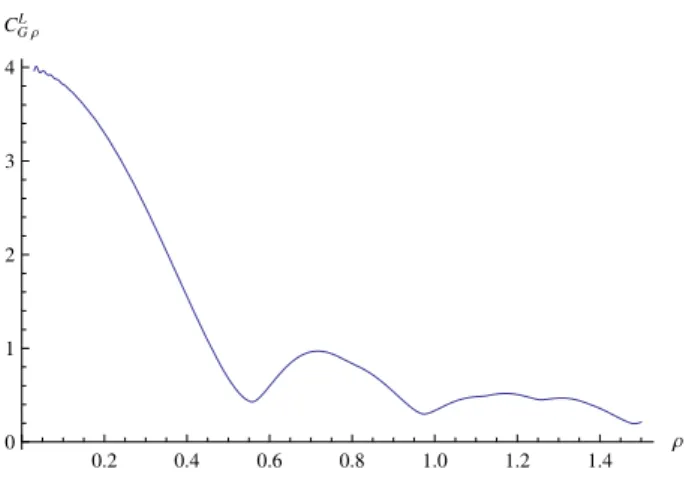
Another grid suitable for length estimation is composed of identical spheres centered in points forming periodic lattice T_{. The grid is for given} lattice type defined by two parameters, the point lattice density and by the spheres diameter. Let us define shape parameterρof the grid equal to the radius of the spheres of the grid homothetically transformed in such a way, that the point latticeT_{is transformed to the unit} latticeS_{. If the grid is randomly rotated the variance} due to orientation of the grid, Var_g∈SO

d(E(estQ|g)),

is obviously zero.

The residual component of variance of the estimate of length of a line segment can be approximated by the variance of the estimate of volume of a cylinder with a diameter equal to the diameter of the spheres in the original grid by a point latticeT_{. The covariogram of} the cylinder can be approximated by a direct product of covariogram of(d ₋1)₋dimensional ball and a line segment. An approximate expression for the residual component of variance of estimate of lengthLof the objectKby the grid of spheres inRd is:

E_g∈SO

d(Var(estL|g))∼=C

L

G(ρ)L(K)SV−1,

CL_G(ρ)=d−1

κd−1

ξ6=0

∑

ξ∈S∗ ξ−d_J2

d−1 2

(2πξ ρ) ,

whereJis the Bessel function of the first kind, follows from the limit transitionSV →∞.

The functionC_GL_(ρ) has a local minimum close to the half of the distance between the nearest lattice

points (Fig. 1), and so the grid of touching spheres shall be effective for the length estimation in 3D.

0.2 0.4 0.6 0.8 1.0 1.2 1.4

Ρ

0 1 2 3 4

CGΡ

L

Fig. 1. Values of C_GL_(ρ) for grid of spheres S with centres in face centered cubic lattice.

In estimates of the curve length the grids of flat planes yield quite different order of asymptotics than grids of curved surfaces, due to increasing curvatures during homothetic downscaling of the curved grids. The variance is also controlled by different properties of the measured object, namely by the total absolute curvature in estimations using parallel surfaces and by the length in estimation by application of spheres.

SURFACE AREA ESTIMATION BY

GRIDS OF STRAIGHT LINES

The surface area of an object in Rd can be estimated from the number of intersection of the object surface with a spatial grid of lines

estS= dκd 2κd−1

N LV

,

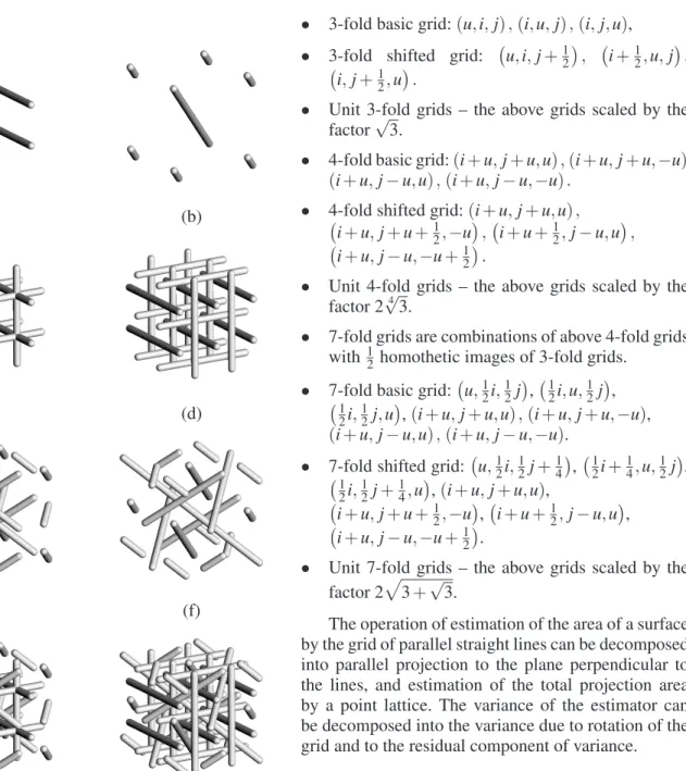
where N is the number of intersections andLV is the length of the grid per unit volume. The grids composed from sets of parallel lines can be used for estimation of the surface area of spatial objects. The estimators can be optimized by finding optimal mutual position of the sets (Kub´ınov´a and Jan´aˇcek,1998). Parametric expressions of two simple grids and three multiple grids in basic and optimized shifted versions (Fig. 2), are listed below, wherei,j_∈Zare discrete parameters,

(a) (b)

(c) (d)

(e) (f)

(g) (h)

Fig. 2. Spatial grids of lines in R3 used for surface area estimation. (a) grid with quadratic cross-section; (b) grid with triangular cross-section; (c) 3-fold basic grid; (d) 3-fold shifted grid; (e) 4-fold basic grid; (f) 4-fold shifted grid; (g) 7-fold basic grid; (h) 7-fold shifted grid.

• Unit grid with quadratic cross-section:(i,j,u)

• Grid with triangular cross-section:(i+u,j+u,u)

• Unit grid with triangular cross-section – the above grid scaled by the factor√43.

• 3-fold basic grid:(u,i,j),(i,u,j),(i,j,u),

• 3-fold shifted grid: ¡u,i,j+1₂¢, ¡i+1₂,u,j¢,

¡

i,j+1₂,u¢.

• Unit 3-fold grids – the above grids scaled by the factor√3.

• 4-fold basic grid:(i+u,j+u,u),(i+u,j+u,₋u),

(i+u,j₋u,u),(i+u,j₋u,₋u).

• 4-fold shifted grid:_¡ (i+u,j+u,u),

i+u,j+u+1 2,−u

¢

,¡i+u+1

2,j−u,u

¢

,

¡

i+u,j₋u,₋u+1 2

¢

.

• Unit 4-fold grids – the above grids scaled by the factor 2√43.

• 7-fold grids are combinations of above 4-fold grids with 1₂ homothetic images of 3-fold grids.

• 7-fold basic grid:¡u,1₂i,1₂j¢,¡1₂i,u,1₂j¢, ¡₁

2i, 1 2j,u

¢

,(i+u,j+u,u),(i+u,j+u,₋u), (i+u,j₋u,u),(i+u,j₋u,₋u).

• 7-fold shifted grid:¡u,1 2i,

1 2j+

1 4

¢

,¡1₂i+1 4,u,

1 2j

¢ , ¡₁

2i, 1 2j+

1 4,u

¢

,(i+u,j+u,u), ¡

i+u,j+u+1₂,₋u¢,¡i+u+1₂,j₋u,u¢, ¡

i+u,j₋u,₋u+1₂¢.

• Unit 7-fold grids – the above grids scaled by the factor 2p3+√3.

The operation of estimation of the area of a surface by the grid of parallel straight lines can be decomposed into parallel projection to the plane perpendicular to the lines, and estimation of the total projection area by a point lattice. The variance of the estimator can be decomposed into the variance due to rotation of the grid and to the residual component of variance.

THE VARIANCE OF SURFACE AREA

ESTIMATES DUE TO ROTATION.

Coefficients of variation of estimate with the grids of lines due to orientationS−1pVar_g∈SO

d(E(estS|g))

Table 1.Coefficient of variation of projection of a flat object into n directions of line grids inR3 calculated using Eq.4from Appendix A.

n CV CV₁2/nCV_n2

1 0.57735 1

3 0.10163 10.8

4 0.07523 14.7

7 0.03822 32.6

Table 2. Coefficient of variation of projection of a cylindrical surface into n directions of line grids inR3

calculated using Eq.5from Appendix A.

n CV CV₁2/nCV_n2

1 0.28418 1

3 0.03706 19.6

4 0.02668 28.4

7 0.01196 80.6

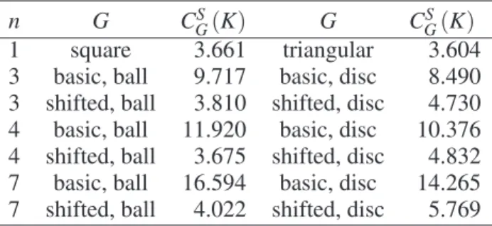
Table 3. Coefficients C_GS(K) in Eq. 3 for residual component of variance of estimates of surface area with unit (LV = 1) line grids G in R3: namely

simple (1) grids with square point lattice cross-section and with triangular point lattice cross-section (K is arbitrary) and multiple (3, 4, 7) basic and shifted grids (K is ball or disc).

n G C_GS(K) G C_GS(K)

1 square 3.661 triangular 3.604

3 basic, ball 9.717 basic, disc 8.490 3 shifted, ball 3.810 shifted, disc 4.730 4 basic, ball 11.920 basic, disc 10.376 4 shifted, ball 3.675 shifted, disc 4.832 7 basic, ball 16.594 basic, disc 14.265 7 shifted, ball 4.022 shifted, disc 5.769

THE RESIDUAL COMPONENT OF

VARIANCE OF SURFACE AREA

ESTIMATES.

The residual component of variance of surface area (S) of objectKestimate by grids of lines inR3can be expressed approximately similarly to Eq.1as

E_g∈SO

3(Var(estS|g)) =C S

G(K)HABS(K)L

−32 V , (3)

where LV is the grid length intensity, HABS(K) is the absolute width of K defined using the absolute mean curvature by equality 2πHABS_=K3

1 (Baddeley,

1980). The values of the coefficients in Eq. 3for our grids (Table 3) and for ball and disc are calculated in Appendix B.

The coefficients of simple grids are independent of the body. In the multiple grids it is not true as demonstrated by the examples of the estimates of the disc and ball surface areas.

DISCUSSION

The study of variances of estimators with periodic grids is important for the design of efficient measurement methods. Approximate asymptotic results for homothetic images of grids with spatial density increasing to infinity, as those applied in the paper to variance of volume estimates or to residual components of variances of the length and surface area estimators, use simple properties of the measured objects and yield useful results for model objects under study. We suppose that the formulas are generally valid, and the coefficients of ball and disc in formula for the residual component of variance of surface area estimates represent extreme values of coefficients for arbitrary objects. Using the knowledge on the behavior of the estimators we were able to design efficient estimators of surface area using spatial grids of shifted line probes and estimators of length of fibre like objects using spatial grids of touching spheres. The asymptotic results are established rigorously in the case of volume estimates only, the theory of variance in more difficult cases – the surface area and length estimates – is far from completness yet, however the presented study with model objects exhibits some important features of the variance of length and surface area estimators.

ACKNOWLEDGEMENT

This study was supported by the Academy of Sciences of the Czech Republic, grants No. A100110502 and AV0Z 50110509.

REFERENCES

Baddeley AJ (1980). Absolute curvatures in integral geometry. Math Proc Camb Phil Soc88:45–58. Baddeley A, Vedel-Jensen EB (2005). Stereology for

statisticians. Boca Raton: Chapman & Hall/CRC. Barbier JE (1860). Note sur probl`eme de l’aiguille et le jeu

du joint couvert. J Math Pure Appl 5:273–87.

Cruz-Orive LM (1997). Stereology of single objects. J Microsc186:93–107.

Hlawka E (1950). ¨Uber Integrale auf konvexen K¨orpern I. Monatsh Math54:1–36.

Jan´aˇcek J (2006). Variance of periodic measure of bounded set with random position. Comment Math Univ Carolinae 47:473–82.

Jan´aˇcek J (2008). An asymptotics of variance of the lattice points count. Czech Math J 58:751–75.

Kiˆeu K, Mora M (2006). Precision of stereological planar area predictors. J Microsc222:201–11.

Kub´ınov´a L, Jan´aˇcek J (1998). Estimating surface area by the isotropic fakir method from thick slices cut in an arbitrary direction. J Microsc191:201–11.

Matheron G (1965). Les variables r´egionalis´ees et leur estimations. Paris: Masson et Cie.

Mattfeldt T, M¨obius H-J, Mall G (1985). Orthogonal triplet probes: an efficient method for unbiased estimation of length and surface of objects with unknown orientation in space. J Microsc139:279–89.

Moran PAP (1950). Numerical integration by systematic sampling. Proc Camb Phil Soc46:111–5.

Santal´o LA (1976). Integral Geometry and Geometric Probability. Reading: Addison-Wesley.

Serra J (1982). Image Analysis and Mathematical Morphology. London: Academic Press.

APPENDIX A

Let us start with auxiliary computations. Let x= (x1, . . .xd),α= (α1, . . .αd),|x|α=|x|α₁1. . .|x|α_dd,|α|=

Σd

i=1αi, then

ˆ

S_d−1|

x_|αdS(x) =

Πd i=1Γ

³

αi+1 2

´

1 2Γ

³

|α|+d

2

´ ,

where dS is surface measure. The equality can be proved by calculating´

Rd|x|αexp

³

−kx_k2

´

dxin two ways: by Fubini theorem and in spherical coordinates.

The indentity´

Sd−11 dS(x) =dκd can serve as an

example whereκd =π

d

2Γ¡d

2+1

¢−1

is the volume of the unit ballBd(1)inRd.

As ´

Sd−1|x1|dS(x) = 2κd−1, the mean of the

projection length of a unit segment to a line (a simple projection) is 2κ_d−1/dκd. As

´

S_d−1|x1|

2

dS(x) =κ_d,

the squared coefficient of variation of the projection is

CV2= µ

dκ_d

2κd−1

¶2

1

d−1.

The values of the the CV2 for d =

1,2,3,4, . . . are 0,π2_{/8−1,1/3,9π}2_{/64−1, . . .} ∼₌

0,0.23,0.33,0.39. . .(the limit isπ/2₋1∼=0.57).

E_g∈SO

d(L1L2), the mixed second order moment

of lengths of projections of a unit segment to two lines spanning angle ψ in R2 (a double projection) is _π1´_φπ₌₀sin|φ₋ψ_|sinφ dφ =

1

π

¡

sinψ+¡π₂₋ψ¢cosψ¢. In Rd we obtain the corresponding value

2

dπ

³

sinψ+³π 2−ψ

´

cosψ´, (4)

multiplying the value for R2 by the value

´

Sd−1

¡

x2₁+x₂2¢dS(x) =2/d.E_g∈SO

d(L1L2), the mixed

second order moment of lengths of projections of unit segments spanning angle χ to corresponding lines spanning angleψ is

ˆ

SOd

|(gy,x) (gu,v)_|dg,

wherex,y,u,v_∈Rd,_|x_|=_|y_|=_|u_|=_|v_|=1,(y,u) = cosψ, (x,v) =cosχ, SOd is the group of rotations equipped with the probabilistic invariant measure. From this formula the kernel Kd can be calculated. Special values ofKdcan be calculated from preceding formulas. Thus CV2 of the simple projection of unit segment gives Kd(0,0) and CV2 of the double projection of a unit segment givesKd(ψ,0). It is easy to see thatK2(ψ,χ) =K2(ψ−χ,0).

By Parseval equality for harmonic analysis onSd−1

we obtain the following expression:

2

π ˆ π₂

ψ=0

K3(ψ,χ)dψ= µ

dκd 2κd−1

¶2

×

Σ∞_n=0(4n+1) µ

(2n₋3)!! (2n+2)!!

¶2µ

(2n₋1)!! 2n!!

¶2

×

Σm l=−m

(2n−2l−1)!! (2n+2l)!!

(2n+2l−1)!!

(2n₋2l)!! cos(2lχ)−1, (5)

which enables us to calculate the variance of multiple projections of a cylindrical surface in R3. It was obtained from Fourier series in spherical harmonics of absolute value of sine of lattitude, of 1₋dimensional measure supported by equator and of sum of Dirac measures locatedχ radians apart from each other.

APPENDIX B

of such euclidean motions of the lines, that the both lines intersect the body, multiplied by the sine of angle between the lines, or the limit for parallel lines. The value for a pair of parallel lines is equal to mean isotropic point covariogram of the planar projection of the body. For nonparallel lines we obtained so far a simple result for ball or disc only. For ball we obtained mont´ee of covariogram of the circle (Matheron,1965). For disc we obtained mont´ee of mean covariogram of the disc planar projection multiplied by 2_π¡sinψ+¡π₂₋ψ¢cosψ¢ where ψ is angle between the lines. Using Poisson summation formula yields the following formulas for coefficients in Eq.3of the ball (as inJan´aˇcek,1999) and the disc (Table 3).

The Fourier coefficient of aaZ3– periodic measure

µ with indexξ _∈a−1Z3,a>0, is

e

µ_ξ =a−3 ˆ

h0,a)3

exp(₋2πixξ)dµ(x) , (6)

C_GS(ball) = 4

π2

ξ₆=0

∑

ξ∈a−1_Z3

¯

¯eµ_ξ¯¯2_|ξ_|−3 .

Fourier coeficients of unit grid with quadratic cross-section are µe_ξ =1 for ξ = (i,j,0), i,j ∈ Z, e

µ_ξ =0 otherwise.

Grid with triangular cross-section:

• µe_ξ =√3 forξ= (i,j,₋i₋j),i,j_∈Z • µe_ξ =0 otherwise.

Coefficients of unit grid with triangular cross-section are √1

3 multiples of above coefficients with indicesξ

scaled by factor √41₃.

3-fold basic grid:

• µe_ξ =1 for ξ = (l,m,0), ξ = (m,0,l) and ξ = (0,l,m).

• µe_ξ = 2 for ξ = (l,0,0), ξ = (0,l,0) and ξ = (0,0,l).

• µe_ξ =3 forξ = (0,0,0).

• µe_ξ =0 otherwise. 3-fold shifted grid:

• µe_ξ = (₋1)m for ξ = (0,l,m), ξ = (m,0,l) and

ξ = (l,m,0).

• µe_ξ =2 for ξ = (2l,0,0),ξ = (0,2l,0) and ξ = (0,0,2l).

• µe_ξ =3 forξ = (0,0,0).

• µe_ξ =0 otherwise.

Coefficients of unit 3-fold grids are 1₃ multiples of above coefficients with indicesξ scaled by factor √1

3.

4-fold basic grid:

• µe_ξ =√3 forξ = (l,m,n)wherel,m,n∈Z\ {0_},

l₆=_±m₆=_±n₆=l, l+m+n=0, l+m₋n=0,

l₋m+n=0 orl₋m₋n=0.

• µe_ξ =2√3 for ξ = (l,₋l,0), ξ = (l,0,₋l), ξ = (0,l,₋l),ξ = (0,l,l),ξ = (l,0,l)andξ= (l,l,0).

• µe_ξ =4√3 forξ = (0,0,0). 4-fold shifted grid:

• µe_ξ =√3 forξ = (l,m,n)wherel,m,n_∈Z\ {0},

l₆=_±m₆=_±n=₆ l,l+m+n=0.

• µe_ξ= (₋1)m√3 forξ= (l,m,n)wherel+m₋n= 0.

• µe_ξ= (₋1)l√3 forξ= (l,m,n)wherel₋m+n= 0.

• µe_ξ= (₋1)n√3 forξ = (l,m,n)wherel₋m₋n= 0.

• µe_ξ =2√3 for ξ = (2l,₋2l,0), ξ = (2l,0,₋2l),

ξ = (0,2l,₋2l),ξ = (0,2l,2l),ξ = (2l,0,2l)and

ξ = (2l,2l,0).

• µeξ =4

√

3 forξ = (0,0,0).

Coefficients of unit 4-fold grids are 1

4√3 multiples

of above coefficients with indices ξ scaled by factor

1 2√43.

7-fold basic grid:

• µe_ξ =4 for ξ = (2l,2m,0), ξ = (2m,0,2l) and

ξ = (0,2l,2m)wherel,m∈Z\ {0},l6=m.

• µe_ξ =8 for ξ = (2l,0,0), ξ = (0,2l,0) and ξ = (0,0,2l).

• µe_ξ =√3 forξ = (l,m,n)wherel,m,n_∈Z\ {0},

l₆=_±m₆=_±n₆=landl+m+n=0,l+m₋n=0,

l₋m+n=0 orl₋m₋n=0.

• µeξ=4+2

√

3 forξ= (2l,₋2l,0),ξ= (2l,0,₋2l),

ξ = (0,2l,₋2l),ξ = (0,2l,2l),ξ = (2l,0,2l)and

ξ = (2l,2l,0).

• µe_ξ = 2√3 for ξ = (2i+1,₋2i+1,0), ξ = (2i+1,0,₋2i+1), ξ = (0,2i+1,₋2i+1), ξ = (0,2i+1,2i+1), ξ = (2i+1,0,2i+1) and ξ = (2i+1,2i+1,0)wherei_∈Z.

• µe_ξ = (₋1)m4 forξ = (2l,2m,0), ξ = (2m,0,2l) andξ = (0,2l,2m)wherel,m_∈Z\ {0_},l₆=m.

• µe_ξ =8 for ξ = (4l,0,0), ξ = (0,4l,0) and ξ = (0,0,4l).

• µe_ξ =√3 forξ = (l,m,n)wherel,m,n_∈Z\ {0_},

l₆=_±m₆=_±n=₆ l,l+m+n=0.

• µe_ξ= (₋1)m√3 forξ= (l,m,n)wherel+m₋n= 0.

• µe_ξ= (₋1)l√3 forξ= (l,m,n)wherel₋m+n= 0.

• µeξ= (−1)n

√

3 forξ = (l,m,n)wherel₋m₋n= 0.

• µe_ξ = (₋1)l4+2√3 for ξ = (2l,₋2l,0), ξ = (2l,0,₋2l), ξ = (0,2l,₋2l), ξ = (0,2l,2l), ξ = (2l,0,2l)andξ= (2l,2l,0).

• µeξ=12+4

√

3 forξ = (0,0,0).

Coefficients of unit 7-fold grids are ¡

4¡3+√3¢¢−1 multiples of above coefficients with

indicesξ scaled by factor ³

2p3+√3 ´₋1

.

We can see that the shifting caused vanishing of the coefficients with smallest indices, which explains the superior performance of the shifted grids (Table 3).

Properly grouping the terms in expression for the coefficients we can use the Epstein zeta functions

Z(A,3)defined as

Z(A,s) = n6=0

∑

|An|−s ,

with matrixAequal toId,d=1 or 2, the identity matrix inRdand

A2=

√

2

4√₃

µ √ 3 2 0 1 2 1 ¶ .

The values of coefficientsCS_G(ball)are

• _π42Z(I2,3)for simple grid with quadratic

crossection,

• 4

π2Z(A2,3)for simple grid with triangular

crossection,

• 4

π2

√ 3

3 (3Z(I2,3) +6Z(I1,3)) for basic 3-fold grid

and ball,

• _π42

√ 3 3

¡

3Z(I2,3)₋9₂Z(I1,3)¢ for shifted 3-fold grid and ball,

• π42

1 23

3 4

³

4_·3−34_Z(_A2,3) +₁₂·₂−32_Z(_I1,3)

´ for basic 4-fold grid and ball,

• 4

π21₂3 3 4

³

4_·3−34_Z(_A2,3)−9·2−32_Z(_I1,3)

´ for shifted 4-fold grid and ball,

• 4

π2 1

2√3+√3

³

4_·314Z(A₂,3) +6Z(I₂,3) +

+3 ³

4+3√2+√6 ´

Z(I1,3)´for basic sevenfold grid and ball,

• 4

π2 1

2√3+√3

³

4_·314Z(A₂,3) +6Z(I₂,3)−

−94

³

4+3√2+√6 ´

Z(I1,3)´ for shifted sevenfold grid and ball.

The Epstein zeta functions Z(I1,3), Z(I2,3) and Z(A2,3) can be calculated using the following identities valid between the Epstein zeta functions, the Riemann zeta functionζ and Dirichlet functionLp

ζ(s) =

∞

∑

n−s, Lp(s) = ∞

∑

(p_|n)n−s,

where(p_|n)is the Kronecker symbol:

Z(I1,s) =2ζ(s),

Z(I2,s) =4ζ³s

2 ´

L₋4

³_s

2 ´

,

Z(A2,s) =21+2s₃1−4sζ

³_s

2 ´

L₋3

³_s

2 ´

.

The covariances of the simple estimates of the disc surface area must be multiplied by additional factor

f(ψ) = 2_π¡sinψ+¡π₂₋ψ¢cosψ¢ where ψ is angle spanned by tangents to parallel lines of the simple subgrids.

Thus we obtain the values of coefficientsCS_G(disc):

• 4 π2 √ 3 3 ¡

3Z(I2,3) +f

¡_π

2

¢

6Z(I1,3)

¢

for basic 3-fold grid and disc,

• _π42

√ 3 3

¡

3Z(I2,3)₋f¡₂π¢9₂Z(I1,3)¢ for shifted 3-fold grid and disc,

• _π42

1 23

3 4

³

4_·3−34_Z(_A2,3) +

+ f¡arccos1₃¢_·12_·2−32Z(I1,3)

´

for basic 4-fold grid and disc.

• 4

π21₂3 3 4

³

4_·3−34_Z(_A2,3)−

− f¡arccos1₃¢_·9_·2−32_Z(_I1,3)

´

for shifted 4-fold grid and disc.

• 4

π2

1 2√3+√3

³

4·314_Z(_A2,₃) +_6Z(_I2,₃) +

+3³4f¡π₂¢+3√2f¡arccos1₃¢+√6f³arccos√1

3

´´

Z(I1,3))for basic sevenfold grid and disc.

• 4

π2

1 2√3+√3

³

4·314_Z(_A2,₃) +_6Z(_I2,₃)−

−9 4

³

4f¡π₂¢+3√2f¡arccos1₃¢+√6f³arccos√1

3

´´