81
Abstract— Adaptive antenna arrays for radar and
communication applications have been the subject of considerable interest during the last few decades. This paper describes the synthesis method of linear array geometry for side lobe level and null control using the Genetic Algorithm. Genetic Algorithm is an iterative stochastic optimizer that works on the concept of survival of the population values based on the fitness value. An adaptive genetic algorithm has been used in linear array to optimize the excitation levels of the elements resulting in a radiation pattern with minimum side lobe level and desired null position. The algorithm encodes each parameter into binary sequences, called a gene, and a set of genes is a chromosome. These chromosomes undergo natural selection, mating, and mutation, to arrive at the final optimal solution. Two design examples are illustrated to show the optimization of linear antenna array using genetic algorithm. MATLAB simulations are done for performance evaluation.
Index Terms—Linear array, Genetic Algorithm, side lobe,
null, MATLAB .
I. INTRODUCTION
Due to increased usage of electromagnetic spectrum, radiation pattern synthesis techniques, which allow placing of one or more nulls in the pattern in specified directions, are gaining technical importance. Many synthesis methods are concerned with suppressing the Side Lobe Level (SLL) while preserving the gain of the main beam [1]. Other methods deal with the null control to reduce the effects of interference and jamming. In the process of placing nulls at the interference locations, side lobe level increases with respect to the main beam. So in this paper the main aim is to optimize both side lobe level and null depth [2]. Interference signals can be
I.Padmaja, Department of Electronics and communication, Gayatri vidya parishad college of Engineering (e-mail: [email protected]). Vishakhapatnam, India, Mobile No. 9704565800.
N.Bala Subrmanyam, Department of Electronics and Communication, Gayatri vidya parishad college of Engineering, Vishakhapatnam, India, Mobile No.8885043414, (e-mail: [email protected]).
N.Deepika Rani, Department of Electronics and communication Gayatri vidya parishad college of Engineering, Vishakhapatnam, India,, Mobile No.9885797722, (e-mail: [email protected]).
G.Tirumala Rao, Department of Electronics and Communication, Gayatri vidya parishad college of Engineering, Vishakhapatnam, India, Mobile No.9866348693, (e-mail: [email protected]).
suppressed in the arrays by steering nulls and thereby reducing the side lobe levels in those directions while keeping the bore sight direction gain unchanged.
In general the sources of interference are in the side lobe region. A narrow band interference source can be suppressed by imposing a single null in the antenna pattern at the proper angle. A wide band jammer, however appears to cover an angular sector of the pattern and therefore it may be required to null an entire sector. This can be done by closely spaced nulls in the entire jammer sector [3].
In recent years, the bionic algorithm for antenna array pattern synthesis has been extensively studied, which have pushed the further development of array pattern synthesis techniques Genetic Algorithm (GA) are one of bionic algorithm that simulates the mechanism of life evolution. Currently, GA has been applied to minimize the side lobe level peak and to steer the nulls in the prescribed directions by controlling the excitation current amplitudes or phases or locations of elements. In our work Genetic algorithm adjusts the current excitation of each antenna element in order to minimize the total output power in the direction of interfering signals and peak side lobe level [4].
Two simplifications are made to the algorithm. First, digitally-controlled search optimization (GA) of the attenuators is adopted. Second, attenuator weights In are used
with even symmetry about the array centre.
II. SYNTHESISFUNCTION
An antenna array is a configuration of individual radiating elements that are arranged in particular configuration and can produce direction radiation pattern. The array geometry is shown in Fig 1.For a linear antenna array; let us assume that there are 2N isotropic radiators placed symmetrically along the array axis (z-axis). The array factor for this symmetric non uniform excitation level linear array is expressed as
) cos cos( *
2 ) (
1
n N
n
n nkd
I
AF
(1)
In = Attenuator weight at nth element with respect to array
center.
d =spacing between the antenna elements
θ =angle of incidence of electromagnetic plane wave. k =2π/λ
βn =phase excitation at nth element.
Linear Array Geometry Synthesis Using Genetic
Algorithm for Optimum Side Lobe Level and
Null
Here the main beam is steered towards broad side direction. Now, the statement of the problem reduces to apply the genetic algorithm to find the optimum current excitation amplitudes that result the pattern with minimum peak side lobe level and null placement control.
Figure 1:
Diagram of a non uniform excitation level linear antenna array. The objective functions used in the genetic algorithm are selected as
M
n
n AF AF Fitness
1
2 2 0
) (
) ( 1
(2)
Where AF(0) , is the output power in the direction of the
main is beam and AF(n) is the output power in the
direction of interference source. If more than one interference sources are present then the total output power is the product
of powers in the direction of
interferers.
ENDL MNDL
w ESLL MSLL w
Fittness2 1 2 (3)
Where MSLL is the maximum peak side lobe level defined
as
MSLL
max
s
AF
, s denotes the side loberegion, ESLL is expected value of the side lobe level, MNDL is the maximum power at the interference
location,
M
n
n AF MNDL
1
)
( , n is the null direction, n=
(1, 2,……M) where M is the number of interference sources, ENDL is the expected null depth level, w1 and w2 are the
weighting factors. The optimum values of w1 and w2 is
between 0 and 1 [5].
In this paper the GA controls the attenuator weights to enable the Fittness1 to maximum and Fittness2 to minimum. The digital attenuators have B bits. B needs to be as small as possible to reduce the cost of the attenuator but should be large enough to steer the nulls at interference directions. Here in this paper we used B=6.We used 4 out of 6 bits of the attenuator to place the null. The nulling amplitudes are represented by
B
A B a
a a
n b
I
1
2 (4)
Where
B total number of bits in the attenuator=6
A number of attenuator bits used for null rejection=4 [b1 b2…… bp] vector containing nulling bits representing In
III. GENETICALGORITHM
Genetic Algorithm is an iterative stochastic optimizer that works on the concept of survival of the population values based on the fitness value and uses methods based on the principle of natural genetics and natural selection to construct search and optimization procedures that best satisfies a predefined goal. Input to the objective function is known as chromosome and output of the objective function is known as cost when minimizing. In GA, chromosomes are abstract representations of the solution to the problem. One approach to represent the antenna as a chromosome is to discretize its parameters and encode them. Here the decimalization coding is employed to encode excitation level of the elements. An adaptive antenna array has 2NB amplitude setting values in which many correspond to local minima in the total output power. Such a large number of amplitude setting values make random search and impractical to use gradient based algorithms [6]. The three main cores of the algorithm are selection, crossover and mutation (Genetic operators).
Fig 2 shows the flow chart of Genetic Algorithm. The genetic algorithm is summarized as below:
Step 1: The GA begins with an initial population consisting of a matrix filled with random ones and zeros. Each row of the matrix consists of the nulling bits of the digital attenuator for each element placed side by side in an array. The size of the matrix is MxNA.
Step 2: Evaluate the objective function value for each row of the attenuator matrix.
Step 3: Invoke natural selection i.e., select the fittest individuals and place them in the mating pool to generate new offspring. The chromosomes are ranked with highest fitness function value on the top and lowest in the bottom. The bottoms 50% of the chromosomes are discarded as they have the least objective function value.
Step 4: Individuals, so called parents placed in the mating pool, are now allowed to mate using two point crossover. In two point crossover, two crossover points are selected, binary string from beginning of chromosome to the first crossover point is copied from one parent, the part from the first to the second crossover point is copied from the second parent and the rest is copied from the first parent.
Step 5: Now, binary mutation is performed. Random binary mutations alter a certain percentage of the bits in the list of chromosomes. These randomly induced variations allow the GA to try new areas of search space while it converges on a solution. The number of nulling bits to be altered in the list of chromosomes is specified by mutation rate.
z axis
-β2 β1 -β1 β2 -β3
GENETIC ALGORITHM
RECEIVER
θ Array centre
d
βI33 I2 I1 I1 I2 I3
83
Figure 2:
Flow chart of Genetic Algorithm
Step 6: After the mutations take place, the fitness values associated with the offspring and mutated chromosomes are calculated, and the process is repeated.
Step 7: This generation process is repeated until a termination condition, a cost that is lower than an acceptable minimum, is reached
IV. RESULTS
The genetic algorithm outlined is applied to broad side linear antenna array consisting of 20 and 48 elements with 0.5λ spacing. The objective is to suppress the output at the interference locations in the antenna radiation pattern while maintaining the side lobe level at -20 dB by controlling the current excitation of radiating elements using 6 bit digital attenuators.
Following examples demonstrate the effectiveness of genetic algorithm for synthesizing single and double nulls. In these examples we assumed ESLL=-20dB and ENDL=-90 dB and weighting factors w1 and w2 is 0.9 and 0.1
respectively.
A. Example 1:
Radiation pattern is computed for 20 element non uniform excitation level linear array with 0.5λ spacing. In this example we assumed interference location at θ=14.23800
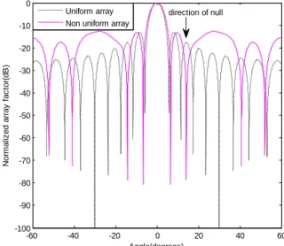
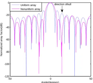
which corresponds to 2nd peak side lobe of the uniform array radiation pattern. Imposing nulls at the interference direction tends to decrease the reduction in side lobe level with respect to main beam there by we have to control the side lobe level also. By adjusting the 4 least significant bits of the attenuator the perturbed patterns for the genetic algorithm are shown in Fig 3-4. Fig 3 corresponds to placing null at the interference location with a null depth of -78.7 dB but the peak side lobe level degraded to -12.74 dB. Fig 4 corresponds to the control of both side lobe level and null control in the antenna array. In this the peak side lobe level is optimized to -19.8dB with a null depth of -73.92 dB with the excitation levels shown in Fig 4. By comparing the perturbed patterns with the uniform array radiation pattern we can observe that there is a slight shift at the interference location i.e., in the GA applied new pattern the interference location is away from the peak of the 3rd side lobe level with a minimal component and this is negligible.
-60 -40 -20 0 20 40 60
-100 -90 -80 -70 -60 -50 -40 -30 -20 -10 0
Angle(degrees)
N
o
rm
a
li
z
e
d
a
rr
a
y
f
a
c
to
r(
d
B
)
Uniform array Non uniform array
direction of null
Figure 3: Normalized radiation pattern for 20element symmetric uniform linear array (dotted line) and for non uniform array (solid line) with 0.5λ spacing having interference signal at θ=14.23800 without peak side lobe level control.
Initialize the search space i.e., fill the attenuator matrix with binary
1’s and 0’s.
The fitness value corresponding to the each chromosome of attenuator matrix
is computed.
The chromosomes are sorted based on their fitness value in ascending order and the best half
chromosomes are selected and remaining half chromosomes are discarded.
From selected top half chromosomes mating process is done to generate the new
chromosomes.
Random binary Mutation is performed.
The discarded chromosomes are replaced with newly generated
chromosomes.
Test fitness value for convergence
Keep Best Individual Yes
Define the objective function
-50 0 50 -120
-100 -80 -60 -40 -20 0
Angle(degrees)
N
o
rm
a
li
z
e
d
a
rr
a
y
f
a
c
to
r(
d
B
)
Uniform array Nonuniform array
direction ofnull
Figure 4: Normalized radiation pattern for 20 element symmetric uniform linear array (dotted line) and for non uniform array (solid line) with 0.5λ spacing with interference signal at θ=14.23800 and optimized peak side lobe level.
Figure 5: Excitation levels for 20 element symmetric non uniform linear array which correspond to radiation pattern fig-4.
B. Example 2:
In this example we considered 48 element uniform linear array 0.5λ spacing. We assumed two interfering signals at θ=5.81550
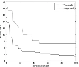
and θ=8.3380 which correspond to the 2nd and 3rd side lobe peaks of the uniform linear antenna array radiation pattern. Implementing the genetic algorithm by adjusting the 4 least significant bits of the digital attenuator the synthesized patterns are shown in Fig 6-7.Fig6 shows the synthesized pattern of the antenna array for the two interference signals with null depths of-77.85 & -64.85 dB but the main lobe to side lobe level ratio degraded to -12.98dB for the excitation levels shown in Fig 8.From Fig-7 we can observe nulls with depths of -64.97 & -48 dB with maximum side lobe level optimized to -20.03dB. Fig 9 shows the convergence of fitness function for optimizing both null control and side lobe level. Fig 10 shows the null depth variation with number of iteration for only null control.
-30 -20 -10 0 10 20 30
-90 -80 -70 -60 -50 -40 -30 -20 -10 0
Angle(degrees)
N
o
rm
a
li
z
e
d
a
rr
a
y
f
a
c
to
r(
d
B
)
Uniform array Non uniform array
direction of nulls
Figure 6: Normalized radiation pattern for 48 element symmetric uniform linear array (dotted line) and for non uniform array (solid line) with 0.5λ spacing having interference signals at θ=5.81550 and θ=8.33650 without peak side lobe level control
-30 -20 -10 0 10 20 30
-100 -90 -80 -70 -60 -50 -40 -30 -20 -10 0
Angle(degrees)
N
o
rm
a
liz
e
d
a
rr
a
y
f
a
c
to
r(
d
B
)
Uniform array Non Uniform array
direction of nulls
Figure 7: Normalized radiation pattern for 48 element symmetric uniform linear array (dotted line) and for non uniform array (solid line) with 0.5λ spacing with multiple nulls at θ=5.81550 , θ=8.33650 and optimized peak side lobe level.
85
0 20 40 60 80 100
2 4 6 8 10 12 14 16 18 20
Iteration number
F
it
n
e
s
s
v
a
lu
e
Two nulls single null
Figure 9: Convergence of fitness function given by (3) for single and double nulls
0 20 40 60 80 100
20 40 60 80 100 120 140
Iteation number
S
N
R
(d
B
)
Two nulls Single null
Figure 10: Convergence of fitness function given by (2) for single and double nulls
V. CONCLUSIONS
This paper illustrated the application of Genetic Algorithm in designing nonuniform excitation level linear antenna arrays having suppressed side lobes and efficient null control in certain direction by controlling main beam direction. The GA has proven quite successful as an adaptive antenna algorithm for arrays. Using a small population size and high mutation rate helps the GA to quickly place nulls with optimal null depth. The GA algorithm was successfully used to optimize the current amplitudes of the radiators to exhibit an array pattern with suppressed side lobes and null placement in certain directions.
REFERENCES
[1] Aritra Chowdhury, Ritwik Giri, Arnob Ghosh, Swagatam Das, Ajith Abraham and Vaclav Snasel,”Linear Antenna Array Synthesis using Fitness-Adaptive Differential Evolution Algorithm”, IEEE, 2010.
[2] SHANG Fei,CAI Ya-xing,GAO Ben-qing,” A New GA Method for Array Pattern Synthesis with Null Steering”, CEEM’2006/Dalian, pp. 490–494.
[3] A. Alphones and V. Passoupatbi, " Null Steering in Phased Arrays by positional Perturbations: A Genetic Algorithm Approach," IEEE International Symposium on Phased Array Systems and Technology, pp. 203 -207, 1996.
[4] Majid M. Khodier, and Christos G. Christodoulou, “Linear Array Synthesis with minimum sidelobe level and Null control using particle swarm optimization,” IEEE TRANSACTIONS ON ANTENNAS AND PROPAGATION, VOL. 53, NO. 8, AUGUST 2005.
[5] Yong-jun Lee,Jong-Woo Seo,Jae-Kwon Ha,Dong-chul park “Null Steering of linear phased Array Antenna Using genetic Algorithm”, IEEE Microwave Conference.,pp. 2726 - 2729 , Dec. 2009 [6] R.L. Haupt, "Phase-only adaptive nulling with genetic algorithms,"
IEEE AP-S Trans., Vol. 45, No. 5, Jun 97, 1009-1015..
I.Padmaja received the B.Tech degree in Electronics and communication engineering from Pragati Engineering College, Jawaharlal Nehru technological university Kakinada, in 2009. She is doing M.Tech in Gayatri vidya Parishad College of engineering in communications and signal processing. She participated in conference on Advances in communication, navigation and computer networks. Her area of interests is in Communications.
N.Bala Subramanyam received the B.E degree in Electronics and Communication Engineering in 1990, M.E degree in Instrumentation and control in 1992, both from
Birla Institute of Technology, Ranchi and Ph.D from Andhra University in June 2006. He is a Professor in the Department of Electronics and Communication, Gayatri Vidya Parishad College of Engineering. His areas of interests include
Microcontrollers and Embedded Systems.
N.Deepika Rani received the B.E degree in Electronics and Communication Engineering in 2000 and the M.E degree in Electronic Instrumentation in 2004, both from AU College of Engineering, Andhra University, Visakhapatnam.
She is an Associate Professor in the Department of Electronics and Communication, Gayatri Vidya Parishad College of Engineering. She is also an Associate member in Institute of Engineers, India. Her research is in the area of fractal antenna engineering.