Volume 36 - Article 28 | Pages 803–850  

VOLUME 36, ARTICLE 28, PAGES 803

−

850

PUBLISHED 16 MARCH 2017

http://www.demographic-research.org/Volumes/Vol36/28/ DOI: 10.4054/DemRes.2017.36.28

Research Article

Measuring male fertility rates in developing

countries with Demographic and Health

Surveys: An assessment of three methods

Bruno Schoumaker

© 2017 Bruno Schoumaker.

This open-access work is published under the terms of the Creative Commons Attribution NonCommercial License 2.0 Germany, which permits use, reproduction & distribution in any medium for non-commercial purposes, provided the original author(s) and source are given credit.

1 Introduction 804

2 Data and methods 805

2.1 Household data and own-children method 806 2.1.1 Linking surviving children with their fathers 807 2.1.2 Estimating age of the father for unmatched children 807 2.1.3 Linking unmatched children (whose fathers are alive) to assigned

fathers

809

2.1.4 Reverse survival of children 810

2.1.5 Computation of male fertility rate 810

2.2 Date-of-last-birth method 812

2.3 Children ever born and the crisscross method 814

3 Comparisons of methods 815

3.1 Comparisons of fertility rates across methods 816

4 Comparisons between male and female fertility 822

5 Conclusion 828

References 830

Measuring male fertility rates in developing countries with

Demographic and Health Surveys: An assessment of three methods

Bruno Schoumaker1

Abstract

BACKGROUND

Levels and patterns of male fertility are poorly documented in developing countries. Demographic accounts of male fertility focus primarily on developed countries, and where such accounts do exist for developing countries they are mainly available at the local or regional level.

OBJECTIVE

We show how data from Demographic and Health Surveys (DHS) can be used to compute age-specific male fertility rates. Three methods are described and compared: the own-children method, the date-of-last-birth method, and the crisscross method. Male and female fertility rates are compared using the own-children method.

RESULTS

Male fertility estimates produced using the own-children method emerge as the most trustworthy. The data needed for this method is widely available and makes it possible to document male fertility in a large number of developing countries. The date-of-last-birth method also appears worthwhile, and may be especially useful for analyzing fertility differentials. The crisscross method is less reliable, but may be of interest for ages below 40. Comparisons of male and female fertility show that reproductive experiences differ across gender in most developing countries: Male fertility is substantially higher than female fertility, and males have their children later than females.

CONTRIBUTION

This study shows that Demographic and Health Surveys constitute a valuable and untapped source of data that can be used to document male fertility in a large number of countries. Male fertility rates are markedly different from female fertility rates in developing countries, and documenting both male and female fertility provides a more complete picture of fertility.

1. Introduction

Male fertility has long been neglected in demographic research (Bledsoe, Guyer, and Lerner 2000; Coleman 2000; Greene and Biddlecom 2000; Tragaki and Bagavos 2014; Zhang 2011). The focus on female fertility is explained by a variety of factors, including the implicit assumption that spouses share identical reproductive interests and behaviors (Greene and Biddlecom 2000), lack of data, quality problems with male fertility data, and the fact that the reproductive age range is less clearly defined for males than for females (Andro and Desgrées du Loû 2009; Estee 2004; Field et al. 2016; Greene and Biddlecom 2000; Paget and Timæus 1994; Ratcliffe, Hill, and Walraven 2000; Zhang 2011). Male fertility data is available in many Western countries through civil registration and vital statistics systems (CRVS), and these have been used in a number of studies on male fertility in developed countries (Brouard 1977; Dudel and Klüsener 2016; Lognard 2010; Tragaki and Bagavos 2014; United Nations 2013; Zhang 2011). However, CRVS systems are deficient in many developing countries, and the collection of fertility data in surveys – especially using full birth histories – has to a large extent focused on females.

As a result, male fertility remains largely undocumented, and even simple facts about male fertility – such as male period fertility rates – are lacking in most developing countries. In these countries, demographic accounts of male fertility are mainly available at the local or regional level (Donadjé 1992a; Hertrich 1996; Pison 1982; Pison 1986; Ratcliffe, Hill, and Walraven 2000), or based on data on the number of children ever born (Blanc and Gage 2000; Ezeh, Seroussi, and Raggers 1996; Field et al. 2016; Johnson and Gu 2009; Macro International 1997). These few studies have shown that the levels and patterns of male and female fertility may differ widely (Donadjé 1992b; Donadjé 1992a; Pison 1986; Ratcliffe, Hill, and Walraven 2000). Males and females do not have the same number of children, do not have their children at the same age, and their reproductive experiences can be very different. Their motivations for having children and the determinants of their fertility may also differ across gender, as shown in several Western countries (Tragaki and Bagavos 2014; Zhang 2011). Better documenting of male fertility may thus contribute to the overall understanding of fertility behavior and transitions in developing countries (Ratcliffe, Hill, and Walraven 2000; Zhang 2011).

and the wide age range covered by the own-children method allow for documenting male fertility in many developing countries. Using the own-children method, we illustrate the extent to which male fertility and female fertility differ in selected settings, and briefly discuss the reasons for these differences.

2. Data and methods

The DHS Program (dhsprogram.com) has collected data in more than 90 countries, beginning in the mid-1980s. Three questionnaires are used in the standard DHS survey: a household questionnaire, a questionnaire for women age 15–49, and (in about two-thirds of the surveys) a questionnaire for a subsample of men (usually) aged 15–59.2 Full birth histories are only collected for females. Three types of DHS data can be used to measure age-specific male fertility rates, each using a different method: 1) data on children living in the households, collected in the household questionnaire (own-children method), 2) data collected in the men’s questionnaire on the date of last birth among men (date-of-last-birth method), and 3) data on the number of children ever born among men collected in two successive men’s surveys (crisscross method). The three methods are described in the following section. Table 1 summarizes the type of data needed for each of the three methods, the number of periods and countries for which rates can be computed with DHS data, and the most common age ranges for each of the methods.

2

Table 1: Data available in Demographic and Health Surveys for computing male fertility rates using three methods (as of November 2016)

Method

Own-children Date-of-last-birth Crisscross

Type of data needed for the method

List of children in household surveys, their ages, and the line number (and age) of the father of the children living in the same household. (a) Survival probabilities of children to reverse survive children.

Date of birth of the last child (month and year) among all men (including never married men). (b)

Number of children ever born among all men in two successive surveys (spaced around five years apart). (c)

DHS questionnaires from which information is drawn

Household and women’s questionnaires (d).

Men’s questionnaire. Men’s questionnaire.

Number of cases for which rates can be computed

188 34 67

Number of countries in which rates can be computed

68 28 32

Most common age range 15 and over 15–59 15–59

(a) In early DHS the line number of the father was not collected. These surveys are not included in the count, as their application of the own-children method is less straightforward.

(b) Only surveys where both the year and month of birth are available are included. (c) Only surveys spaced seven years apart or less are included in the count.

(d) Survival probabilities of children are obtained from female birth histories in the women’s questionnaire.

The data used in the own-children method is the most widely available by far (188 periods, 68 countries), and it also covers the largest age range (15 and over). The date of last birth is available in only 34 surveys (28 countries) for males aged 15–59, while the crisscross method can be used to compute fertility rates for 67 periods in 32 countries, again generally for males aged 15–59. The estimates from the own-children and crisscross methods can be compared in the same country and same period in 54 cases, the own-children and date-of-last-birth estimates can be compared in 29 cases, and all three methods can be compared in 11 cases.

2.1 Household data and own-children method

with their mother, 2) to classify the children by their single year of age and by single year of age of the mother, 3) to redistribute unmatched children by age of the mother, 4) to reverse survive the children to estimate the number of births by year and age of the mother, and 5) to reverse survive the female population in the years preceding the survey to estimate the denominator of the rates (Cho, Retherford, and Choe 1986; United Nations 1983). In this article the own-children method is adapted to measure male fertility.3

2.1.1 Linking surviving children with their fathers

Surviving children are linked with their father to obtain the age of the father at birth of the child, as in the standard approach. This is straightforward when the child lives in the same household as the father because the line number of the father is included in DHS data.

2.1.2 Estimating age of the father for unmatched children

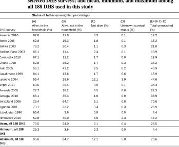
Classifying children and their fathers by single year of age is not straightforward when they do not share the same household or the father is deceased. For these unmatched children the father’s age must be estimated. Table 2 shows the percentage of unmatched children (aged 0–4) in selected surveys, as well as the minimum, maximum, and average in the 188 available surveys. The mean percentage of children not living in the same household as their father is 26.5%. Most of these cases are due to fathers that are alive but not living with their children (24.0%), with the percentage of children with a father who is deceased or has an unknown survival status accounting for a small part of the unmatched children (2.5%). These percentages of unmatched children vary strongly across countries, ranging from less than 5% (Uzbekistan) to 70% (Swaziland), and are much higher for fathers than for mothers. Two changes have been made to the standard approach in order to address the issue of unmatched children.

3

Table 2: Distribution of surviving children aged 0–4 by status of father, for 16 selected DHS surveys; and mean, minimum, and maximum among all 188 DHS used in this study

Status of father (unweighted percentage)

DHS survey

(A) Alive, in the household (%)

(B) Alive, not in the household (%)

(C) Not alive (%)

(D) Unknown survival status (%) (E=B+C+D) Total unmatched (%)

Armenia 2010 87.8 11.8 0.3 0.1 12.2

Benin 2006 82.8 15.3 1.8 0.1 17.2

Bolivia 2003 78.2 20.4 1.1 0.3 21.8

Burkina Faso 2003 86.1 11.4 2.4 0.1 13.9

Cambodia 2010 87.1 11.2 1.7 0.0 12.9

Ghana 1998 62.8 35.2 1.7 0.3 37.2

Haiti 2005 56.1 41.2 2.5 0.2 43.9

Kazakhstan 1999 84.1 13.6 1.7 0.6 15.9

Lesotho 2004 55.4 28.6 12.1 3.9 44.6

Nepal 2011 63.6 35.4 0.9 0.1 36.4

Rwanda 2005 77.7 18.2 3.5 0.6 22.3

Senegal 2010 63.1 35.3 1.6 0.0 36.9

Swaziland 2006 29.4 64.7 5.1 0.8 70.6

Uganda 2001 73.1 23.2 3.4 0.3 26.9

Uzbekistan 1996 95.6 3.6 0.8 0.0 4.4

Zimbabwe 2010 52.8 40.0 4.9 2.3 47.2

Mean, all 188 DHS 73.5 24.0 2.1 0.4 26.5

Minimum, all 188 DHS

29.3 3.6 0.3 0.0 4.4

Maximum, all 188 DHS

95.6 64.7 12.1 5.8 70.6

In the standard approach to estimating female fertility, unmatched children of a given age x are redistributed by age of the mother a using the same distribution of mothers’ ages reported for matched children the same age. In other words, the mothers of unmatched children of agex are assumed to have the same age distribution as the mothers of matched children of agex. In this paper we relax this assumption by using random hot deck imputation (Allison 2001) to estimate the age of surviving fathers who do not live in the household.

Before imputing the age of fathers, children whose fathers are not alive are dropped from the list of surviving children.4 In this way, only children who could have been reported by their fathers at the time of the survey – if their fathers had been interviewed – are included. This step is important for two reasons: 1) the age of the

4

deceased fathers at the time the children were born does not need to be estimated, and 2) reverse surviving the males in the years preceding the survey is unnecessary and data on male adult mortality is not required. In this process we assume that male fertility is independent of male mortality. The impact of this assumption on recent fertility is small, given the small percentage of children aged 0–4 with deceased fathers (Table 2).

Age of the father for children whose father is alive is imputed in the following way: for each unmatched child, a child with the same characteristics (age and age of mother)5 is randomly selected among matched children.6 The age of the father of the selected child is assigned to the father of the unmatched child. While the standard approach considers the age distribution of fathers of matched children and unmatched children of agex to be the same, using the mother’s age in the imputation process leads to a lower age at birth (one year on average) for fathers of unmatched children compared with fathers of matched children.7

2.1.3 Linking unmatched children (whose fathers are alive) to assigned fathers

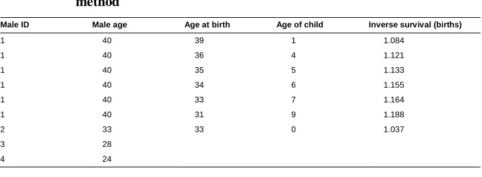
The next step consists of ‘finding a father’ for unmatched children. In this process, a man the same age as the imputed age of the (living) father is randomly selected from the men in the household data set, whether or not the man is already a father. This linkage is an artifice that allows construction of a data file for men and their surviving children that can be manipulated and used in various ways.8 The file contains all the adult men, with one or more lines per man: one line for men with no children or with one surviving child, and multiple lines for men with several surviving children (Table 3). Men can have several children of the same age, and these children can be born from the same mother or from different mothers.

5 _{If age of the mother is also missing, it is first imputed with random hot deck imputation based of the age of}

the child and the place of residence.

6

Random imputation is performed ten times, and ten series of age-specific male fertility rates are computed. Average fertility rates based on the ten series are reported.

7

Other information, such as the type of place of residence, could also be taken into account in the imputation, but including additional information has a very limited impact on the results.

8

Table 3: Illustration of individual data file for the adapted own-children method

Male ID Male age Age at birth Age of child Inverse survival (births)

1 40 39 1 1.084

1 40 36 4 1.121

1 40 35 5 1.133

1 40 34 6 1.155

1 40 33 7 1.164

1 40 31 9 1.188

2 33 33 0 1.037

3 28

4 24

Male ID: identification of male

Male age: male’s completed age at the time of the survey Age at birth: completed age of the father at birth of the child Age of child: child’s completed age at the time of the survey

Inverse survival: inverse of the survival probability of the child to completed age. Represents the number of births corresponding to a surviving child.

2.1.4 Reverse survival of children

Children of completed agex are reverse survived to estimate the number of births x years before the survey. Survival probabilities of children are computed directly from female birth histories collected in DHS surveys. The survival probability between birth and completed agex is computed as the proportion of children born xyears before the survey that are alive at the time of the survey. Births are then estimated by multiplying the surviving children by the inverse of the survival probability corresponding to their age. For example, each surviving child aged 1 year represents 1.084 births for the period one to two years ago (Table 3).

2.1.5 Computation of male fertility rates

over the preceding five years.9 Age-specific male fertility rates are computed by dividing births by exposure.

The quality of male fertility estimates with the own-children method depends primarily on two factors, the assumptions described above and the quality of the data. The quality of data collected through the household questionnaire may be affected by problems also found in female birth histories – underreporting of young children and artificial aging of young children (Schoumaker 2014a) – which lead to underestimating fertility. On the other hand, slight overestimation of fertility may occur if non-biological fathers report orphans as own children, but this effect is expected to be very limited given the low percentages of orphans in most countries. In addition, a strength of the own-children method over the two other methods is that children can be reported and included in fertility rates even if their fathers are not aware of their existence, which limits downward bias resulting from fathers’ lack of awareness of progeny. As a result, we expect the own-children estimates to be comparable to estimates that would have been produced with birth histories. Comparisons of own-children estimates with direct estimates from birth histories among females show that they are indeed very similar (Avery et al. 2013), and we expect this to hold for males also. Another advantage of the own-children method is that fertility rates can be computed over a broad age range, since data is collected on all the members of the household regardless of their age. Finally, the sample size is larger for the own-children method than for the two other methods (based on a subsample of men), and should lead to less variable estimates.

The special case of polygyny is briefly discussed, as it is a factor in the differences between male and female fertility. The method described above allows for dealing with children from polygynous unions in the same way as children from monogamous unions (and children born to women not in a union). In this sense, there is no specific treatment for polygynous unions. If the children live in the same household as their father, they are linked with their father in a straightforward way. If the children do not live with their father – as is the case when the man’s various spouses do not live in the same household – the age of the father will have to be imputed and the children will be matched randomly to a man of the same age as the imputed age.10 The imputed age of the father will be based on the age of the mother, as described above.11 This approach,

9 _{Only completed age is available in the household survey. The birthdates of men are imputed by subtracting}

the completed age from the date of the survey (month and year), and subtracting again a random number of months between 0 and 11 drawn from a uniform distribution.

10

From an aggregate perspective (e.g., the computing of fertility rates among all males), it does not matter that the child is not linked to his/her actual father. What is important is that the child is linked to a father with the same characteristics as his/her father.

11

however, cannot be used to compare the fertility rates of polygynous men with those of monogamous men. In that case it would be necessary to link unmatched children to fathers of the same marriage type (e.g., polygynous) as their actual father. The lack of data on the number of wives of men and on the number of cowives of women makes this difficult.

2.2 Date-of-last-birth method

A second method for estimating male fertility rates is the date-of-last-birth method. Data for implementing the date-of-last-birth method is less readily available in DHS surveys (Table 1) than data for the own-children (OC) method, and the age range for the data that is available is more limited (usually 15–59). Nevertheless, the date-of-last-birth method can be used with a substantial number of DHS surveys and relies on very simple data and methods.

The method uses data on the date of birth (month and year) of the last child reported by men.12 Age-specific fertility rates are computed using the approach developed by Schmertmann (1999). Under the assumption that fertility rates are constant within age groups over a given period (e.g., five years), fertility rates in age group j ( ) are computed as the ratio of the number of visible births (last births) to the visible exposure in that age group in that period:

= (1)

Applying this approach to estimating age-specific male fertility rates, visible exposure in each age group is measured as the sum of the duration (for each man) spent in the age group between the date of the survey and the date of the last birth, or the date of the start of the period if no birth occurred in the period (e.g., five years). In Figure 1 visible exposure is represented by continuous lines.

underestimated. If men in a polygynous union are less likely than monogamous men to live with their children, this could lead to slightly underestimating the mean age at fatherhood.

12

Figure 1: Illustration of visible and invisible exposure, and visible and invisible births with data on date of last birth

Note: Adapted from Schmertmann (1999).

This method relies on the accuracy of the date of last birth. For recent births we expect the date of birth to be fairly accurate. We do not expect systematic displacements of births among males, as the male questionnaire provides no incentive to displace births, contrary to what is found for females (Schoumaker 2014a). The date-of-last-birth method also assumes that fathers report all their biological children (and only their biological children), which is not always the case. We expect underreporting of births to be more common than overreporting as men may not be aware of, or may be reluctant to report, births that occurred out of wedlock. The treatment of multiple births with this method is another source of slight underestimation of fertility, as it relies on the assumption of one birth occurring at a time.13 Therefore, we expect date-of-last-birth fertility rates to be lower than own-children fertility rates.

This paper presents results for all men, regardless of their socioeconomic characteristics or marriage type (e.g., polygyny). However, the date-of-last-birth method also allows for the comparison of male fertility rates among different groups. This is possible because – contrary to the own-children method – the information on fertility is obtained directly from males. It would allow, for instance, comparing fertility rates among polygynous men and monogamous men, as the number of wives is usually collected in the men’s questionnaire in DHS. This method also makes it possible to measure rates by level of education, standard of living, etc.

13

2.3 Children ever born and the crisscross method

Age-specific male period fertility rates can also be computed by comparing data on children ever born, by age, drawn from two successive surveys. This is possible with DHS data in 67 cases (Table 1). The method was developed for estimating female fertility rates in the 1970s and 1980s (Arretx 1973; Coale, John, and Richards 1985; Zlotnik and Hill 1981) and later improved by Schmertmann (2002). As shown by Schmertmann (2002), age-specific fertility rates (λ) between two exact ages (x andx+n) over a period of any length (t) (Figure 2) can be estimated with a simple formula (called ‘crisscross,’ equation 2).

= + . ( − ) + − . ( − ) (2)

whereA, B, C, and D are the mean number of children ever born at exact ages and dates defined by the corners of the rectangle in the Lexis diagram corresponding to the age group and period of the rate,14 t is the time interval between the two surveys, andn is the width of the age group.15

Figure 2: Illustration of Lexis diagram for estimating fertility rates using the crisscross approach

Note: Adapted from Schmertmann (2002).

The crisscross method relies on the availability of at least two surveys containing data on the number of children ever born. Unlike the two other methods (own-children and date-of-last-birth), the crisscross method is not affected by inaccuracies in birth dates or ages of children because it relies on the number of children ever born. If the

14

The mean number of children ever born by exact age is estimated by smoothing the number of children ever born by completed age, using a regression model with restricted cubic splines.

15

same percentages of births are omitted in the two surveys, the method will also not be affected by omissions of births (Schoumaker 2014b). However, the crisscross method is highly sensitive to differential omissions of births across surveys and to differences in sample composition (Schoumaker 2014b; Zlotnik and Hill 1981). Because of the sensitivity to differential data quality, we expect the crisscross method to lead to more variable estimates of age-specific fertility rates than those produced by the other two methods.

As with the two other methods, only aggregate country-level results are presented in this paper. Potentially, this method allows for computing rates for subpopulations, as long as there is no or limited mobility across categories over time.

3. Comparisons of methods

Male fertility rates are computed for five-year periods with the own-children and date-of-last-birth methods (own-children, date-date-of-last-birth) and for periods of between five and seven years with the crisscross method.16 All the surveys that allow for comparisons between at least two methods are used, and in 11 cases it was possible to compare all three methods for the same country and period. The own-children and crisscross methods are compared in 54 cases (including the 11 cases with the three methods); the own-children and date-of-last-birth estimates are compared in 29 cases (including the 11 cases with the three methods). In total, comparisons across methods are possible for 72 cases (54+29–11) in 35 countries.

These comparisons have several objectives. The first is to identify the method that is best suited for documenting male fertility at the country level, i.e., the method that is available in a large number of cases and is able to provide trustworthy estimates for a wide age range. The second is to evaluate the reliability of male fertility estimates. A high degree of consistency across methods for the same cases suggests that the estimates are trustworthy. The third – related – objective is to evaluate whether the different methods lead to similar results and whether, as a result, one method can be used in place of the others. This is useful if only one type of data is available in a specific survey or census. It is also valuable when analyzing fertility differentials. For instance, the date-of-last-birth method is potentially better suited than the own-children method to compute fertility estimates for subpopulations. Showing that these two methods provide similar estimates at the country level is thus a key step before proceeding to the use of date-of-last-birth estimates for fertility differentials.

16

3.1 Comparisons of fertility rates across methods

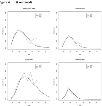
Figures comparing age-specific male fertility rates across methods are presented in Appendix Figure A-1 for the 72 cases. Selected cases are presented below to illustrate the main results (Figure 3 and Figure 4). These comparisons are complemented with scatterplots (Figure 5, Appendix Figures A-2–A-4) and boxplots (Figure 6) that summarize the differences across methods.

Figure 3: (Continued)

Figure 5: Scatterplots of age-specific male fertility rates and total fertility rates using three methods – own-children (OC), date-of-last-birth (DLB), and crisscross (CC) – with DHS data

(a) (b)

(c) (d)

First, different methods provide consistent estimates in a substantial number of cases (Figure 3, Figure 4, Appendix Figure A-1). For instance, date-of-last-birth and own-children estimates are very close in Kenya and Kazakhstan (Figure 3); curves of age-specific fertility rates are also close for the own-children and crisscross methods in several cases, such as Cambodia and Armenia (Figure 4). Even when the estimates do not match perfectly, the shapes are fairly similar in a number of cases (Brazil, Nicaragua, Zimbabwe, Figure 3; Madagascar, Figure 4). However, despite similarities, these figures indicate some clear differences across methods. Of the three methods, the own-children estimates show the most regular and plausible curves for age-specific fertility rates (Figure 3, Figure 4, Appendix Figure A-1). By contrast, crisscross estimates are highly erratic in some cases (e.g., Madagascar 2006, Guinea 2002, Figure 3), and negative rates are even found in a number of cases, reflecting differential data quality across surveys. Overall date-of-last-birth curves appear much more regular than crisscross estimates, but less plausible than own-children estimates in some cases (e.g., Zimbabwe 1992, Figure 3; Ethiopia 1990, Appendix Figure A-1).

As shown by the scatterplots of age-specific fertility rates (all ages combined, Figure 5a, Figure 5c, Figure 5e), the correlation between own-children rates and date-of-last-birth rates (r=0.96) is much stronger than the correlation of these rates with crisscross rates (r=0.72 for own-children-crisscross, r=0.64 for crisscross-date-of-last-birth). The correlation between own-children rates and date-of-last-birth rates is also strong within all age groups (Appendix Figure A-2), while the crisscross rates are poorly correlated with rates from the other methods above age 40 (Appendix Figure A-3 and Appendix Figure A-4). While the correlations of crisscross age-specific rates with rates from the other methods are lows, correlations for total fertility rates (15–54) are much better (Figure 5b, Figure 5d, Figure 5f), but still lower that the correlations between own-children total fertility rates and date-of-last-birth total fertility rates.

Scatterplots also show that date-of-last-birth estimates tend to be lower than own-children estimates. While estimates from different methods should be located along the line of identity (X=Y), date-of-last-birth rates and total fertility rates are on average below that line (Figure 5a, Figure 5b). This is also visible in the boxplots (Figure 6a).17 Each boxplot summarizes the ratios of rates across methods (e.g., the date-of-last-birth rate divided by the own-children rate) by age group. The medians of these ratios (the band inside the box) should be close to 1, meaning the two methods lead on average to similar results. The bottom and top of the box (first and third quartile) and the whiskers indicate the variability of these ratios, which should ideally be low. Ratios of date-of-last-birth rates to own-children rates (Figure 6a) tend to be lower than 1, especially at young ages (below 25) and above 45. The lower date-of-last-birth estimates suggest that births are underreported by men when asked about the date of birth of their last child.

By contrast, crisscross estimates do not appear to be systematically below or above own-children estimates (Figure 6b). The variability of ratios of rates is very large below 20 and above 40, but for most of the age range (20 to 54 years), crisscross estimates are, on average, close to own-children estimates. For a specific country, crisscross rates are thus poor estimates because of their large variability, but the fact that crisscross rates are, on average, close to own-children rates suggests that own-children rates and crisscross rates are on average closer to the true values than date-of-last-birth rates.

Figure 6: Boxplots of ratios of age-specific male fertility rates (date-of-last-birth vs. own-children, crisscross vs. own-children, date-of-last-(date-of-last-birth vs. crisscross) with DHS data

a. Date-of-last-birth vs. Own-children b. Crisscross vs. Own-children

c. Date-of-last-birth vs. Crisscross

In summary, the own-children rates appear to be the most trustworthy, cover the widest age range, and are available in the largest set of surveys and countries. Date-of-last-birth rates are strongly correlated with own-children rates and the ratios of rates do not vary strongly, but date-of-last-birth rates tend to be lower than own-children rates (by 15% on average). The strong correlation between these two methods (regardless of age) indicates that even though they do not provide exactly the same rates, the patterns documented by these two methods are fairly similar. The lower estimates for the date-of-last-birth method are consistent with more frequent underreporting of births with that method than with the own-children method. Despite the probable underestimation of the date-of-last-birth estimates, they may be especially useful for measuring fertility differentials if underreporting of births does not vary strongly across categories of men. The rates produced by the crisscross method appear to be less valuable because of the large variability of rates reflecting differential data quality across surveys. The crisscross method is thus not recommended for documenting fertility at all ages. However, comparisons across methods show that crisscross estimates may be useful between ages 20 and 40, where crisscross rates are fairly consistent with rates estimated using the two other methods.

4. Comparisons between male and female fertility

In this last section we use own-children estimates to compare male and female fertility rates in a variety of settings.18 These comparisons show that reproductive behavior may differ greatly between males and females, and that in developing countries large differences across gender are the norm rather than the exception.

Age-specific fertility rates are presented for males and females in six selected countries from various parts of the world, with varying levels of fertility and polygyny (Figure 7). Male and female quantum and tempo indicators (total fertility rates19 and mean ages at fatherhood/motherhood) are also computed for 188 surveys in 68 countries (Figure 8). These comparisons confirm that men start their reproductive lives later than women (lower rates at young ages) and extend their reproductive career over a longer period, with higher rates at older ages (Paget and Timæus 1994; Pison 1986; Zhang 2011). In monogamous settings with relatively low fertility, such as Kazakhstan and Cambodia (Figures 7a and 7b), age-specific fertility rates are only slightly different, and total fertility rates are a little higher among males (Estee 2004; Zhang 2011). In

18

For the sake of comparison, the own-children method is also used to compute age-specific female fertility rates. These rates are very close to the direct estimates from birth histories, as already shown in previous research (Avery et al. 2013).

polygynous societies such as Mali and Niger (Figures 7e and 7f), differences between males and females are much greater. Males start their reproductive life significantly later than women and continue having children well beyond age 60. These differences also translate into very large differences in total fertility rates. For instance, the male total fertility rate in Mali (2010) is 10.4, compared to 6.4 among females, while in Niger (1989) these figures are 12 and 7. These results clearly illustrate that reproductive experiences can vary greatly by gender not only at the local level, as documented in several rural areas in West African countries (Donadjé 1992b; Pison 1986; Ratcliffe, Hill, and Walraven 2000), but also at the country level. Male and female fertility may also differ substantially in countries where polygyny is limited but where males have their children much later than females, as in Rwanda and Haiti (Figures 7c and 7d).

Figure 7: Comparisons of age-specific period fertility rates among males and females in six countries with varying levels of fertility and polygyny. Fertility computed using the own-children method with DHS data

Low fertility, no polygyny

(a)

Polygyny: 1.2% of married men Male total fertility rate: 2.2 Female total fertility rate: 2.1 Mean age at fatherhood: 29.3 Mean age at childbearing: 26.4

(b)

Figure 7: (Continued)

Medium fertility, low polygyny

(c)

Polygyny: 2.9% of married men Male total fertility rate: 6.3 Female TFR: 4.1

Mean age at fatherhood: 37.8 Mean age at childbearing: 30.3

(d)

Polygyny: 6.7% of married men Male total fertility rate: 5.1 Female total fertility rate: 3.8 Mean age at fatherhood: 37.0 Mean age at childbearing: 30.9

High fertility, high polygyny

(e)

Polygyny: 22.1% of married men Male total fertility rate: 10.4 Female total fertility rate: 6.3 Mean age at fatherhood: 41.6 Mean age at childbearing: 29.6

(f)

Polygyny: 23.5% of married men Male total fertility rate: 12.0 Female total fertility rate: 7.0 Mean age at fatherhood: 41.8 Mean age at childbearing: 29.6

The level of polygyny is measured as the percentage of married men with more than one spouse.

The apparent inconsistencies between male and female total fertility rates have been discussed previously in several papers (Field et al. 2016; Pison 1982; Vallin and Caselli 2001). These differences in total fertility are related to the large differences in the age at which men and women have their children, and to the differences in the number of men and women at the ages when they have their children (Field et al. 2016; Vallin and Caselli 2001). The differences in the number of men and women in turn depend mainly – when migration is limited – on the population growth rate and on the differences in survival to these ages.

The stable population model20 is useful to illustrate the factors influencing the differences between male and female fertility. In a stable population the male total fertility rate (TFRM) is related to the female total fertility rate (TFRF) in the following way (see Appendix for details):

TFRM_=TFRF_∙ 1 SRB∙

( )

( )∙exp r∙(TM−TF) (3)

whereSRB is the sex ratio at birth (ratio of males to females), p(MAC) and p(MAF) are the survival probabilities from birth to the mean age at childbearing (females) and at fatherhood (men), r is the population growth rate, and TM and TF are the mean length of generation for males and females. The mean length of generation is not equal to the mean age at childbearing (or fatherhood), but is closely related to these measures (Preston, Heuveline, and Guillot 2001).

Rearranging equation 3 by computing the ratio of male and female total fertility rates and taking natural logs on both sides gives:

ln TFR_TFRMF =ln _SRB1 +ln ₍( )₎ +r∙(TM−TF) (4)

This equation shows that differences in total fertility rates between males and females are related to the differences between age at fatherhood and age at motherhood in two ways. First, the difference in the mean length of generations between males and females (TM–TF) will – if positive and combined with a growing population – lead to a larger total fertility rate among males. Secondly, the survival probability to the mean age at childbearing among females will be greater than the survival probability to the age at fatherhood among males, both because female mortality is usually lower than male mortality and because the age at fatherhood is greater than the age at childbearing. In summary, large age differences between spouses, combined with high growth rates, will be accompanied by large differences in total fertility rates between males and females.

20

This situation is found in many sub-Saharan African countries, where male total fertility rates are often 1.5 to 2 times greater than female total fertility rates. This will often be accompanied by polygyny, although this is not a necessary condition for these large differences between male and female fertility (Field et al. 2016). By contrast, in cases where the mean age at fatherhood and the mean age at childbearing are close, the differences between the total fertility rates will be small.

It is beyond the scope of this paper to reconcile male and female total fertility. In nonstable populations, the relationships between male and female total fertility will be more complex than those described by equation 4; for instance, if changes in the age– sex distribution are rapid or if the population pyramid is affected by migration. Equation 4 is thus not directly applicable to our data. However, the strong empirical correlation (r=0.91) between the natural logarithm of the ratios of male to female total fertility rates (left-hand side of equation 4) and the difference between mean age at fatherhood and mean age at childbearing (Figure 9) confirms that large differences in ages at childbearing and fatherhood go hand in hand with large differences in total fertility.21

21

Figure 8: Comparisons of male total fertility rates (15–79) and female total fertility rates (15–54) in 188 surveys (68 countries) and comparisons of mean age at childbearing and mean age at fatherhood in the same 188 surveys. Fertility computed using the own-children method with DHS data

(a) Total fertility rate (TFR)

Figure 9: Relationship between the natural logarithm of the ratio of male TFR to female TFR and the difference between mean age at fatherhood and mean age at childbearing, in 188 surveys (68 countries). Fertility computed using the own-children method with DHS data

5. Conclusion

This paper compares three methods of measuring age-specific male fertility rates using DHS data. The own-children method is the most promising for this purpose. It provides the most-trustworthy estimates, allows the documenting of male fertility rates in a large number of countries with existing data, and covers the broadest age range. The date-of-last-birth method can also be useful. Although our results suggest it underestimates male fertility, the date-of-last-birth approach can be a straightforward way of obtaining worthwhile male fertility estimates at low cost, especially for measuring fertility differentials. The crisscross method is less valuable than the other two methods, but it can be used to measure age-specific fertility rates for ages 20 to 40 or to estimate total fertility rates when neither of the other two methods is available.

References

Allison, P.D. (2001).Missing data. Thousand Oaks: SAGE (Quantitative Applications in the Social Sciences 136).

Andro, A. and Desgrées du Loû, A. (2009). La place des hommes dans la santé sexuelle et reproductive: Enjeux et difficultés. Autrepart 52(4): 3–12.doi:10.3917/autr. 052.0003.

Arretx, C. (1973). Fertility estimates derived from information on children ever born using data from censuses. In: Proceedings of the IUSSP International Population Conference. Liège: Ordina: 247–261.

Avery, C., St. Clair, T., Levin, M., and Hill, K. (2013). The ‘own children’ fertility estimation procedure: A reappraisal. Population Studies 67(2): 171–183.

doi:10.1080/00324728.2013.769616.

Blanc, A. and Gage, A. (2000). Men, polygyny, and fertility over the life-course in sub-Saharan Africa. In: Bledsoe, C., Lerner, S. and Guyer, J. (eds.).Fertility and the male life-cycle in the era of fertility decline. New York: Oxford University Press: 163–187.

Bledsoe, C., Guyer, J., and Lerner, S. (2000). Introduction. In: C. Bledsoe, S. Lerner, and J. Guyer (eds.).Fertility and the male life-cycle in the era of fertility decline. New York: Oxford University Press: 1–26.

Brouard, N. (1977). Evolution de la fécondité masculine depuis le début du siècle. Population (French Edition)32(6): 1123–1158.doi:10.2307/1531392.

Cho, L.-J., Retherford, R., and Choe, M. (1986).The own-children method of fertility estimation. Honolulu: University of Hawaii Press/East-West Center Population Institute.

Coale, A.J., John, A.M., and Richards, T. (1985). Calculation of age-specific fertility schedules from tabulations of parity in two censuses. Demography22(4): 611– 623.doi:10.2307/2061591.

Coleman, D. (2000). Male fertility trends in industrial countries: Theories in search of some evidence. In: Bledsoe, C., Lerner, S. and Guyer, J. (eds.).Fertility and the male life-cycle in the era of fertility decline. Oxford: Oxford University Press: 29–60.

Donadjé, F. (1992b). Nuptialité et fécondité des hommes au Sud-Bénin: Faits et opinions.Cahiers Québécois de Démographie 21(1): 45–65. doi:10.7202/0101 04ar.

Dudel, C. and Klüsener, S. (2016). Estimating male fertility in eastern and western Germany since 1991: A new lowest low?Demographic Research35(53): 1549– 1560.doi:10.4054/DemRes.2016.35.53.

Estee, S. (2004). Natality: Measures based on vital statistics. In: Siegel, J. and Swanson, D. (eds.).The methods and materials of demography. 2nd edition. Amsterdam: Elsevier: 371–405.

Ezeh, A., Seroussi, M., and Raggers, H. (1996).Men’s fertility, contraceptive use, and reproductive preferences. Calverton: Macro International (DHS Comparative Studies 18).

Field, E., Molitor, V., Schoonbroodt, A., and Tertilt, M. (2016). Gender gaps in completed fertility. Journal of Demographic Economics 82(2): 167–206.

doi:10.1017/dem.2016.5.

Greene, M.E. and Biddlecom, A.E. (2000). Absent and problematic men: Demographic accounts of male reproductive roles.Population and Development Review26(1): 81–115.doi:10.1111/j.1728-4457.2000.00081.x.

Hertrich, V. (1996). Permanences et changements de l’Afrique rurale: Dynamiques familiales chez les Bwa du Mali. Paris: CEPED (Les Études du CEPED 14).

Johnson, K. and Gu, Y. (2009). Men’s reproductive health: Findings from Demographic and Health Surveys, 1995–2004. Calverton: ICF Macro (DHS Comparative Reports 17).

Lognard, M.-O. (2010). L’évolution de la fécondité masculine en Belgique de 1939 à 1995. In: Eggerickx, T. and Sanderson, J.-P. (eds.).Histoire de la population de la Belgique et de ses territoires: Actes de la Chaire Quetelet 2005. Louvain-la-Neuve: Presses universitaires de Louvain: 527–546.

Macro International (1997). The male role in fertility, family planning, and reproductive health. Calverton: Macro International.

Paget, W.J. and Timæus, I.M. (1994). A relational Gompertz model of male fertility: Development and assessment.Population Studies 48(2): 333–340.doi:10.1080/ 0032472031000147826.

Pison, G. (1986). La démographie de la polygamie.Population (French Edition)41(1): 93–122.doi:10.2307/1533182.

Preston, S., Heuveline, P., and Guillot, M. (2001). Demography: Measuring and modeling population processes. Oxford: Wiley-Blackwell.

Ratcliffe, A.A., Hill, A.G., and Walraven, G. (2000). Separate lives, different interests: Male and female reproduction in the Gambia. Bulletin of the World Health Organization78(5): 570–579.

Schmertmann, C.P. (1999). Fertility estimation from open birth-interval data. Demography36(4): 505–519.doi:10.2307/2648087.

Schmertmann, C.P. (2002). A simple method for estimating age-specific rates from sequential cross sections. Demography 39(2): 287–310.doi:10.1353/dem.2002. 0018.

Schoumaker, B. (2014a). Quality and consistency of DHS fertility estimates, 1990 to 2012. Rockville: ICF International (DHS Methodological Report 12).

Schoumaker, B. (2014b). The crisscross method to evaluate data quality in fertility surveys. Paper presented at the 2014 Annual Meeting of the Population Association of America, Boston, May 1–3, 2014.

Tragaki, A. and Bagavos, C. (2014). Male fertility in Greece: Trends and differentials by education level and employment status. Demographic Research 31(6): 137– 160.doi:10.4054/DemRes.2014.31.6.

United Nations (1983). Manual X: Indirect techniques for demographic estimation. New York: United Nations, Department of Economic and Social Affairs, Population Division (Population Studies 81).

United Nations (2013).Demographic Yearbook 2012. New York: United Nations.

Vallin, J. and Caselli, G. (2001). Le remplacement de la population. In: Caselli, G., Vallin, J., and Wunsch, G. Démographie: Analyse et synthèse, tome I: La dynamique des populations. Paris: INED/PUF: 403–419.

Zhang, L. (2011). Male fertility patterns and determinants. Dordrecht: Springer (Springer Series on Demographic Methods and Population Analysis 27).

doi:10.1007/978-90-481-8939-7.

Appendix: Relationship between male and female total fertility rates

in stable populations

The approximate link between the male TFRs and the female TFRs is explained in the case of a stable population. The intrinsic growth rate (r) in a stable population is related to the net reproduction rate among females (NRRF) in the following way (Preston, Heuveline, and Guillot 2001):

r

=

TF (A1)

where TF is the mean length of generation among females (Preston, Heuveline, and Guillot 2001). Rearranging this formula and taking the exponential of both sides, we have:

NRRF_=exp(r∙TF_{) (A2)}

The net reproduction rate is also approximated by the following formula (Preston, Heuveline, and Guillot 2001):

NRRF=TFRF∙ 1

1+SRB∙p(MAC) (A3)

where TFRF is the total fertility among females, SRB is the sex ratio at birth (ratio of male births to female births), and p(MAC) is the probability of surviving from birth to the mean age at childbearing (MAC).

Substituting the expression for NRR (A3) into A2 gives:

TFRF∙ 1

1+SRB∙p(MAC) =exp(r ∙T ) (A4)

Among males, we have the following equations:

NRRM_=exp(r∙TM_{) (A5)}

NRRM=TFRM∙ SRB

And finally:

TFRM∙ SRB

1+SRB∙p(MAF) =exp(r ∙T ) (A7)

where TFRM is the total fertility among males, p(MAF) is the probability of surviving from birth to the mean age at fatherhood (MAF), and TM is the mean length of generation among males.

Dividing A7 by A4 gives:

TFRM TFRF∙SRB∙

p(MAF) p(MAC) =

∙

∙ (A8)

Rearranging A8, we find:

TFRM=TFRF∙ 1

SRB∙ p(MAC)

P(MAF)∙exp r∙ T M