Numerical application of Adomian decomposition method to fifth-order autonomous differential equations

J. Math. Comput. Sci. 7 (2017), No. 3, 554-563 ISSN: 1927-5307

NUMERICAL APPLICATION OF ADOMIAN DECOMPOSITION METHOD TO FIFTH-ORDER AUTONOMOUS DIFFERENTIAL EQUATIONS

E. U. AGOM1,∗_{, F. O. OGUNFIDITIMI}2_{, P. N. ASSI}1

1_{Department of Mathematics, University of Calabar, Calabar, Nigeria}

2_{Department of Mathematics, University of Abuja, Abuja, Nigeria}

Copyright c2017 E. U. Agom, F. O. Ogunfiditimi and P. N. Assi. This is an open access article distributed under the Creative Commons

Attribution License, which permits unrestricted use, distribution, and reproduction in any medium, provided the original work is properly cited.

Abstract.In this paper, Adomian Decomposition Method(ADM) is applied to Fifth-Order autonomous differential

equations. The general concept of ADM to this class of equations was stated in relation to the general concept.

Three test problems were used to validate the concept of the decomposition method, and the result in series form

of only the first six terms were obtained. The absolute error were also obtained, similarly the plots of both the

exact and ADM solutions. The series form solution by ADM gave almost the same result as those obtained

by any known closed form method of the continuous function. Thus, justifying the excellent potentials of the

decomposition method.

Keywords:fifth-order autonomous differential equations; Adomian decomposition method.

2010 AMS Subject Classification:65L05.

1. Introduction

∗_{Corresponding author}

E-mail address: [email protected]

Received November 8, 2016; Published May 1, 2017

Fifth-order Differential equations generally arise in modeling of visco-elastic flow. The exis-tence and uniqueness of the solution to this class of linear autonomous differential equation is common everywhere [9]. Also, variation of parameter is applied to the linear case of this class of equations. For the nonlinear class of these equations, numerical methods are applied. Previ-ous numerical methods applied to problems of visco-elastic flow are finite difference method, finite element method and finite volume method. In this paper, we explore the possibility of using the ADM in obtaining the solution to fifth-order autonomous differential equation.

Although the solution of the decomposition method is also an approximation, but it is one that does not change the problem. The method itself has some features in common with other methods. But, it is distinctly different on closer examination and it offers several significant advantages. For details on ADM see [2], [3], [4], [5], [7] and [10]. The general fifth-order differential equation is given as

dnξ

dtn = f(t,ξ,ζ,α,β,γ), n=5 (1)

where

ζ = dξ

dt ,α= d2ξ

dt2,β = d3ξ

dt3,γ = d4ξ

dt4

And f(t,ξ,ζ,α,β,γ)is a continuous function oft,ξ,ζ,α,β andγ in some region.

2. Concept of ADM

ADM Consider equation (1.1) to be of the form

ξ−N(ξ) = f(t) (2)

where N is a nonlinear operator and zero in this case with regards to equation (1.1). f(t) is a known function and seeks the solution ξ satisfying equation (1.1). We assume that for every f, equation (2.1) has one and only one solution. The ADM consist of approximating equation (2.1) as an infinite series.

ξ =

∞

∑

n=0

and

N(ξ) =

∞

∑

n=0 A_n(t)

(4)

whereA_n(t)is known as the Adomian polynomial given as

A_n(t) = 1 n!

dn

dλn[N(

∞

∑

i=0

λiξi(t))]λ=0

(5)

Where n = 0, 1, 2, ... andλ is a grouping parameter. For details of equation (2.4) see [8] and [11]. The proof of convergence of equations (2.2) and (2.3) are given in [1] and [6].

Substituting equations (2.2) and (2.3) in (2.1), yields

∞

∑

n=0

ξn(t)−

∞

∑

n=0

A_n(t) = f(t)

(6)

From equation (2.5) the iterations are then determined in the following recursive way, where we identify

ξ0(t) = f(t)

ξn+1(t) =An(ξ0(t),ξ1(t),ξ2(t), ...,ξn(t))

Thus, all component ofξ(t)are determined once the Adomian Polynomials are obtained. The polynomials are obtained based on the nonlinear term in the nonlinear functional. The acceler-ated form of this polynomial are given in literature and the usual Adomian form is given by [2]. The nth term approximation of equation (2.1) is given as

φn(ξ) = n−1

∑

i=0

ξi(t) (7)

with

lim_n→∞φn(ξ) =ξ(t)

In the linear case of equation (1.1), the application of ADM is equivalent to a classical itereration method. But the posteriori calculation of the constantL−1is by imposing eachφn(ξ)to verify each initial/boundary condition. In this paper, L is a fifth-order differential and L−1 is a fifth-fold integral which determine a set suitable for good convergence.

In this section, we apply ADM to 5th-order linear autonomous differential equations.

3.1 Problem 1

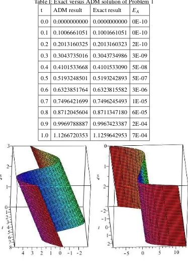
In comparison to equation (1.1), consider

ξ(5)+3γ+4β+4α+3ζ+ξ =0 ξ =ξ(t), tε[0,1]

and

ξ(0) =ξ

00

(0) =ξ(iv)(0) =0, ξ

0

(0) =ξ

000

(0) =1 The exact solution is

ξ(t) =e−t(2+3t+t2)−2 cost Using the equations (2.1) through (2.6), we have

ξ0=t+ t3

6 ξ1=−

7t5

120−

t6

144−

t7

1680−

t8

40320 ξ2=

7t6

240+ 43t7

5040+ 19t8

13440+ 19t10

181440+

t11

2217600+

t12

79833600+

t13

6227020800

Proceeding in this order we obtain ξ5(t), the ADM result ofξ(t) =∑5_i=0ξi(t)and exact result are shown in Table 1. With only 6 terms of the series solution considered the absolute error(E_A)

3.2 Problem 2

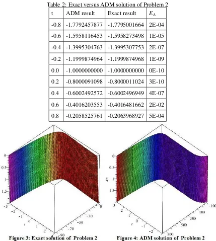
Also, in comparison to equation (1), consider

ξ(5)+5γ+10β+10α+5ζ+ξ =0 ξ =ξ(t), tε(−1,1) and

ξ(0) =−1,ξ

0

(0) =1,ξ

00

(0) =ξ(iv)(0) =ξ

000

(0) =0.

The exact solution is

ξ(t) =e−t

−1+t 2 2 + t3 3 + t4 8

Applying the equations (2.1) through (2.6), we have ξ0=−1+t

ξ1=− t5

30−

t6

720 ξ2=

t6

36+

t7

117+ 5t8

4032+ t9 12096+ t10 403200+ t11 39916800 ξ3=−

5t7

252− 85t8

8064− 5t9

2016−

t10

3024−

109t11

3991680−

23t12

15966720−

17t14

17435658240 − t 13 20756736− t15 93405312000− t16 20922789888000

Table 2: Exact versus ADM solution of Problem 2 t ADM result Exact result EA -0.8 -1.7792457877 -1.7795001664 2E-04 -0.6 -1.5958116453 -1.5958273498 1E-05 -0.4 -1.3995304763 -1.3995307753 2E-07 -0.2 -1.1999874964 -1.1999874968 1E-09 0.0 -1.0000000000 -1.0000000000 0E-10 0.2 -0.8000091098 -0.8000011024 3E-10 0.4 -0.6002492572 -0.6002496949 4E-07 0.6 -0.4016203553 -0.4016481662 2E-02 0.8 -0.2058525761 -0.2063968927 5E-04

3.3 Problem 3

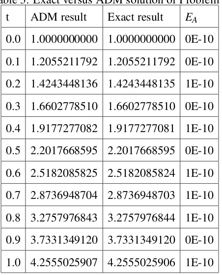
Similarly, in comparison to equation (1), consider

ξ(5)−2β+ζ =0 ξ =ξ(t), tε[0,1] and

ξ(0) =1,ξ

0

(0) =2,ξ

00

(0) =1,ξ

000

The exact solution is

ξ(t) =4−e

−t

4 (9+3t)−

et

4 (3−5t)

Also, applying the equations (2.1) through (2.6), we have

ξ0=1+2t+ t2

2 +

t3

2 + 5t4

24 ξ1=

t5

30+

t6

80−

t7

1680−

t8

8064

Proceeding in this order we obtainξ5(t). The ADM result ofξ(t) =∑5i=0ξi(t)and exact result are shown in Table 3. With only 6 terms of the series solution considered the absolute error

(EA)is also very very minimal as shown in Table 3. These is also obvious in Figures 5 and 6.

Table 3: Exact versus ADM solution of Problem 3 t ADM result Exact result E_A

4. Conclusion

In this paper, we have successfully applied ADM to 5th order linear autonomous differential equations. The introduction consisted of real life areas were 5th differential equations are used as models. Followed by, the numerical methods that are often used for solving this class of equations and an overview of ADM. We also gave the general ADM for this class of equation and applied to concrete examples. The results were fantastic, nearly the same as those obtained by classical method. Although, we all know that in real life problems the laws of nature are nonlinear and stochastic in general. As such, one of the most relevant features of ADM is that the matching procedures are not necessary.

Conflict of Interests

The authors declare that there is no conflict of interests.

REFERENCES

[1] K. Abaoui and Y. Cherruault, Convergence of Adomian’s Method Applied to Differential Equations. Comput.

Math. Appl. 5 (1994), 103-109.

[2] G. Adomian, Solving Frontier Problems of Physics: the Decomposition Method. New York,NY, USA:

Springer, 1993.

[3] E. U. Agom and F. O. Ogunfiditimi, Numer. Application of Adomian Decomposition Method to One

[4] E. U. Agom and F. O. Ogunfiditim, Numer. Solution of Third Order Time-Invariant Linear Differential

Equa-tions by Adomian Decomposition Method, Int. J. Eng. Sci. 5 (2016), 81-85.

[5] E. U. Agom, F. O. Ogunfiditim and A. Tahir, Numer. Solution of Fourth Order Linear Differential Equations

by Adomian Decomposition Method , Br. J. Math. Comput. Sci. 17 (2016), 1-8.

[6] A. Ahmed, Convergence of Adomian Decomposition Method for Initial-Value Problems. Numer. Method for

Partial Differential Equations, 27 (2011), 749-752.

[7] A. Almazmumy, F. A. Hendi, H. O. Bakodah and H. Alzumi, Recent Modifications of Adomian

Decomposi-ton Method for Initial Value Problems in Ordinary Differential Equations. Am. J. Comput. Math. 2 (2012),

228-234.

[8] J. Biazar, E. Babolian, A. Nouri and S. Islam. An Alternative Algorithm for Computing Adomian Polynomials

in Special cases. Appl. Math. Comput. 138 (2003), 523-529.

[9] N. O. Sadata, Existence Solution for 5th Order Differential Equations under some Conditions, Appl. Math. 1

(2010), 279-282.

[10] N. Sigh and M. Kumar, Adomian Decomposition Method for Solving Higher-Order Boundary Value

Prob-lems, Math. Theory Modelling, 2 (1) (2011), 11-22.

[11] A. M. Wazwaz, A New Algorithm for Calculating Adomian Polynomials for Nonlinear Operator, Appl. Math.