http://www.sciencepublishinggroup.com/j/fm doi: 10.11648/j.fm.20170305.11
Analytical and Numerical Calculation of the Orifice
Minimum Temperature Due to Joule - Thomson Effect
Mohammed Mohammed Said, Abdelrahem Dohina, Lotfy Hassan Rabie
Mechanical Power Engineering Department, Faculty of Engineering, Mansoura University, El-Mansoura, Egypt
Email address:
[email protected] (M. M. Said), [email protected] (A. Dohina), [email protected] (L. H. Rabie)
To cite this article:
Mohammed Mohammed Said, Abdelrahem Dohina, Lotfy Hassan Rabie. Analytical and Numerical Calculation of the Orifice Minimum Temperature Due to Joule - Thomson Effect. Fluid Mechanics. Vol. 3, No. 5, 2017, pp. 33-43. doi: 10.11648/j.fm.20170305.11
Received: June 7, 2017; Accepted: June 19, 2017; Published: August 16, 2017
Abstract:
High pressure drop generated by a restriction orifice may result in a very low temperature, which can affect the piping material and may cause catastrophic piping failure if the operating temperature becomes lower than the minimum design temperature. This minimum design temperature is stated by piping ASME B31.3 code as -48°C. In such piping research branch, there has been relatively little investigation of very low temperature effect on pipelines. As well as, sizing the orifice with implementing temperature control to match piping material has a few analytical explanations, particularly in investigating the influence of Joule - Thomson effect on piping damage. Most commercial orifice sizing software ignore Joule - Thomson effect even though in choked flow condition. The objective of the present research is to compare a derived analytical equation with 3-D computational calculations by using ANSYS 16.0 for Joule - Thomson temperature drop through the orifice. As well as correlate the analytical equation to be safely considered as a good prediction tool for the lowest temperature at orifice throat instead of misleading ISO 5761 fully developed Joule - Thomson temperature drop. The analytical equation correlation has been carried out based on non-linear regression by grouping flow conditions, fluid properties, and orifice geometry, for minimum temperature prediction at orifice Vena-contracta. The numerical temperature differences in the fully developed flow regime after the office have been compared with EN ISO 5761-Part 3 Joule - Thomson temperature drop equation. Three orifices with β ratios, 0.3, 0.4, and 0.5 have been chosen for such study and numerical simulations have be carried out using k-ε and k-ω turbulence models. As a corollary of this study, it was concluded that the k-k-ε and k-ω models predict well both the flow and the fully developed temperature drop as compared with ISO 5761 equations. The errors are generally accepted at all conditions and both values give good agreement. The derived equation successfully predicts the lowest minimum temperature at Vena-contracta and can supersede ISO 5761-Part 3 Joule - Thomson temperature drop at fully devolved region.Keywords: ANSYS 16.0, ISO 5761, Joule-Thomson Coefficient, Low Temperature Material, Orifice, Turbulence
1. Introduction
Restriction orifice is common used in gas processing facilities, which may have flare or vent systems that occasionally handle cold relief flows. As the fluid flow passes through the restricted orifice, a significant pressure drop is created across the orifice plate which results in high pressure loss [1]. Hence, the pressure drop through orifices always undergoes several research studies. From such studies is the investigation of the pressure drop through orifices for single and two phase flow [2]. Where the pressure drop correlated equations for both the single phase Idel’chick et al. and two phase Morris and Simpson et al. have been investigated and adopted in this study. A
compressible gas is subjected to high-pressure consideration, however regarding to the downstream portion ignoring the low temperature effect may lead to piping material selection misconception. In the design phase, an engineer may select a pipe so that it can be used at a lower temperature. One solution is to use special cold temperature-rated steels in pipes. Steel pipes, traditionally used in gas pipeline systems generally conform to API 5L and ASTM 106 B specifications. These are manufactured in several grades and having pressure-temperature rating as well as minimum temperature to define SMYS. Careful reading of ASME B31.3 reveals that the minimum temperature for A106B is at 244°K (-29°C), depending on the thickness of pipe. The temperature drop increases with the increase of the pressure drop and is proportional to Joule-Thomson coefficient [4]. The cooling due to the Joule - Thomson effect may be greater than the warming from ambient conditions through the relieved piping. Therefore, the main objective of this study is to investigate numerically the induced - maximum temperature drop due to Joule - Thomson effect in throttling application and to validate by such numerical results the maximum temperature ratios of a derived analytical equation to supersede the fully developed temperature drop in EN ISO 5761. Most studies that exist for predicting orifice Joule - Thomson effect in orifice plate application are focusing only on flow measurement correction and are rarely dealt with in commercial software of orifice sizing. Moreover, Joule - Thomson coefficient validation studies have been less considered and even ignored in orifice related standards. In many instances, determination of orifice Joule - Thomson coefficient is essential to compensate for measured fully developed downstream temperature and consequently correct for flow measurement. The accuracy of such measurement with respect to pressure drop is characterized by Joule - Thomson effect in [4]. The study presents a procedure to enable the compensation of Joule - Thomson effect in natural gas flow-rate measurements. It has been derived in [5] a numerical procedure for the calculation of the natural gas specific heat capacity, the isentropic exponent, and the Joule - Thomson coefficient that can be used to compensate for the adiabatic expansion effects in real - time flow rate measurements. The results showed that the procedure can be efficiently applied in both off-line calculations and real time measurements. The effect of a Joule - Thomson expansion on the accuracy of natural gas flow rate measurements was pointed out in [6]. The study investigated the computationally intensive procedure for the precise compensation of the flow rate error, caused by the Joule - Thomson expansion effects. In the present study methane gas is the adopted fluid and the uncertainty Joule - Thomson coefficients at different operating pressures for methane are extracted from experimental figures in [7]. Joule - Thomson coefficient equation has been reported in EN ISO 5761 standard and the temperature reduction is assigned only with fully developed flow at 5D to 15D downstream the orifice [8]. Hence the maximum
temperature drop close to the orifice, in the standard and elsewhere, has not been investigated yet. EN ISO 5761 restricts temperature calculation at the throat only if the gas is in the vicinity of its dew - point and the temperature at the throat may be calculated assuming an isentropic expansion from the upstream conditions. Due to difficulty of measuring orifice temperature at throat and with an increased accuracy in numerical modeling over the years, it is now plausible to use it for flow - temperature induced conditions where experimental data are not available. Due to orifice sizing by EN ISO 5761-2 equation is an iterative approach, it was investigated in [9] a new equation to calculate the mass flow rate with the aid of thermodynamic fundamentals. The equation is explicit and no rather becomes iterative due to expansion factor and discharge coefficient dropping from the new derived equation. The mass flow rate results are within ± 0.4%. At the present study, the numerical solution has been carried out using ANSYS 16.0 software and compared, for the sake of accuracy, with a derived equation for Joule - Thomson temperature drop. Also the validation of the numerical approach has been investigated for the restricted orifice (DN 50) fully developed temperature drop by comparing the calculated data to that predicted by EN ISO 5761-2 Joule - Thomson temperature drop equation. Moreover, the present numerical study will focus on three main cases of distinct boundary conditions. Both first and second cases include three different boundary conditions of inlet and outlet pressures while the third includes three different geometries with fixed inlet and outlet pressure boundary conditions. Unsteady 1-D (one-dimensional) temperature distribution in the DN 50 (2 inches) pipe, upstream and downstream of the orifice was investigated by OpenFOAM 2.3.x CFD model in [3]. Choked flow case was studied and compared with Aker’s results by Olga simulation tool. The results showed that a minimum pipe temperature of 191.8°K (-81.2°C) was obtained and compared to Aker’s 177.1 °K (-95,9°C). CFD simulation have been performed by OpenFOAM 1.6 and validated by published experimental data to predict orifice flow [10]. The results showed a successful agreement for flow pattern, energy balance, pressure recovery and both velocity and pressure profiles. At the present study 3-D two-equation k-ε and k-ω models are adopted for turbulence closure. The k-ε model is used as it becomes an industrial standard and it is comparatively cheap to run and gives acceptable results in many cases, however k-ω is a more recent entrant to the industrial CFD arena, and outline the distinguishing features of other models that are beginning to make an impact on industrial turbulence modelling [11]. Finally, with the previous critical effects of minimum design temperatures emerging from restricted orifice application, authors felt necessary to propose a numerically validated equation for minimum temperature perditions in orifice throttling application.
Orifice is mainly sized in gas application by very simple formula which often referred to as the “Basic Compressible Sizing Equation” which is expressed by Equation (1) [12, 13], and can be derived easily using Bernoulli Theorem. As shown in Fig. 1, P, is the inlet static pressure measured at D upstream the orifice, P, is the outlet static pressure measured at ½ D downstream the orifice, hence in Equation (1),
∆P = P − P.
Where q , is the mass flow rate, and C, is the discharge coefficient [8, 14]. The discharge coefficient is the ratio of the mass flow rate through the orifice to the theoretical maximum mass flow rate [14].
q = Y d 2∆Pρ (1)
The increase in kinetic energy is at the expense of not only the potential energy (pressure), but also the internal energy (temperature) of the fluid as expressed by Equation (2) [15]. Elsewhere in the present study, for sake of validation, the mass flow results by ISO Equation (1) will be denoted
q (ISO) and compared with the numerical mass flow rate results denoted q (CFD).
∆T = (2)
2.1. Analytical Model for Minimum Temperature
2.1.1. En ISO 5761-2 Model
The principle of the method of measurement is based on the installation of an orifice plate into a pipeline in which a fluid is running full. The presence of the orifice plate during compressible gas expansion causes both static pressure and temperature to change between the upstream and downstream sides of the plate. The fully developed pressure drop (∆P ), and temperature drop (∆T ), can be determined using EN ISO 5761 Equations (3) and (4), respectively [8, 14]:
∆P = ∆P (3)
∆T = μ!"∆P (4)
Where, ∆P and ∆T are the pressure loss and temperature drop along a distance of 2D, upstream and 6D, downstream the orifice plate, and μ!", is the Joule - Thomson coefficient. The Joule - Thomson coefficient, μ!" , is determined by using Equation (5)[8] whereas, μ!", represents for real gas rate of change of temperature with respect to pressure at constant enthalpy.
μ!"=#"#$⃒& (5)
As depicted by Equation (4) the temperature drop due to Joule - Thomson effect at fully developed zone, i.e., 6D downstream the orifice, is proportional to the product of, μ!" and the pressure loss, ∆P [4, 14]. For sake of comparison in this study, the Joule - Thomson coefficients have been obtained to be involved in Equation (4) and more information and demonstration for methane Joule - Thomson coefficients
are described in [4].
2.1.2. Analytically Derived Minimum Temperature Ratio
EN ISO 5761 standard estimates only the temperature drop due to orifice throttling at the fully developed region with applying real gas Joule - Thomson coefficient. Lake of information for temperature drop along the full downstream domain leads to incomplete design methodology. Defining the ratio, '""(
)* as the ratio of minimum temperature at orifice throat, T , and the upstream temperature, T . Therefore, it is essential to establish a validated equation to determine the minimum temperature ratio resulting from restriction at the orifice throat. So, all the variable parameters which have a direct influence on the expansion process are identified and by instantaneous solution of mass and energy conservation equations, extended with the thermodynamics equation of state between orifice’s upstream and throat. Upon few mathematical assumptions and applying the polynomial expansion theory for the resulting equation root, an expression for the minimum temperature ratio is derived and can be written in the form of Equation (6). Whereas all subscripts in Equation (6) denoted 1 and 2 are referring to the upstream and throat, respectively. Hence, the equation validity can be investigated by comparing the analytical results from such equation with the numerical perdition results by ANSYS 16.0 at same boundary conditions. These boundary conditions are different inlet pressures, different outlet pressures, and different beta ratios.
'"" (
)*= ' ( +1 +
. / " −
0' ( '11( 2 3045 6 78 93
066 3 05 6 78 3: ; (6)
By discarding non-significant terms, for the sake of simplification in Equation (6), thus a simplified formula is given in the form of Equation (7). In this expression both compressibility factor, Z and specific heat at constant pressure, C= are assumed constant during gas expansion.
ΔT ?@= T ∗ B
' ( C. D
/ " E (7)
For sake of comparison with numerical minimum temperature, T , it is essential to define, T∗, as the minimum temperature which calculated by Equation (8) and expressed as:
T∗= T − ΔT
?@ (8)
2.2. Numerical Model
Both k-ε and k-ω models being used here to obtain the numerical solution to a flow problem for mass flow rate which has been validated by EN ISO 5761 mass flow rate Equation (1). Also, pressure and temperature profiles are obtained to examine the orifice Joule - Thomson characteristic.
2.2.1. Continuity Equation
When conservation of mass over a finite volume of a compressible fluid is considered, the total mass entering the control volume must equal the total mass exiting the control volume (assuming there are no sources/sinks of mass). This leads to the steady state mass-weighted continuity equation in the form of Equation (9) [16].
# GHIJ
#@J = 0 (9) 2.2.2. Momentum Equation
Applying Newton's second law (the rate of change of momentum on an element equals the total forces acting on that element) to a volume of fluid gives the mass weighted momentum Equation (10) [16].
L
L@MCρNuP)uPQD = −
#=H #@J+
#
#@MCτN)Q+ τNNNDSTU (10)
Where τ)Q, is the stress tensor and Reynolds stress tensor, τ)QU is showed by Equation (11) [16].
τSTU
NNN = −ρuNNNNNNNNSˊˊuTˊˊ (11) Equations (10) and (11) are usually referred to the Reynolds averaged Navier-Stokes equations.
2.2.3. Energy Equation
ANSYS solves conservation equations for mass and momentum. For flows involving heat transfer or compressibility, an additional equation for energy conservation is solved. The steady sate energy conservation for expansion flow through orifice can be considered without heat addition neither work done and can be given in the form of Equation (12) [16, 17]
L
L@JCρNuP)HY + ρuS˝H
˝
NNNNNNND = L
L@JCuPQτN)Q+ [NNNNNND\˝τSTU (12)
Where the flow of compressible gas through a restricted orifice is considered isenthalpic without heat addition and no work done. Furthermore, it is assumed that the heat transfer across the pipe wall is adiabatic.
2.2.4. Ansys Meshing
ANSYS 16.0 Workbench meshing tool is used to implement a tetrahedrons unstructured mesh in the stream-wise direction and is gradually refined near to the orifice throat by boundary adaptation within a circular region. The adaptation mesh procedure was followed as recommended in [17]
.
After an initial solution, it was determined that ] values of some of the cells were too large and reached 250 near the orifice walls, and after ] adaption was used to refine them to lay between 20 and 30. The resulting meshesfor all cases showed that the average mesh density is around 1.5x10 elements as depicted in Fig. 2.
2.2.5. Set up and Boundary Conditions
A large source of uncertainty in CFD modeling can result from poor representation of boundary conditions, [18]. Also some flow problems can be very sensitive to apparently minor changes in the boundary conditions or problem geometry. The compressible fluid is a pure methane. For sake of diversity to validate both ISO temperature drop equation (4) and analytically derived equation (7), three main cases including three different sub-cases per each main case, have been solved by ANSYS 16.0. The first main case is corresponding to fixed outlet pressure at 5.0 MPa and three different inlet pressures 8.3 MPa, 6.9 MPa, and 5.5 MPa. Second main case is corresponding to fixed inlet pressure boundary condition at 8.3 MPa with three different outlet pressures at 6.8 MPa, 5.8 MPa, and 4.8 MPa. First and main cases are solved using the k-ε model, with both inlet temperature at 300°K and β, ratio of 0.3. In the third main case the inlet and outlet pressures are 4.9 MPa and 3.0 MPa respectively, is solved by using the k-ω model where the validation is also extended to another constant inlet temperature at 400°K and three different β, ratios of 0.3, 0.4 and 0.5. The orifice is attached to a pipe of inside diameter, 49 mm, and the piping is extended 2D and 6D upstream and downstream the orifice, respectively.
3. Results and Discussion
All the numerical results are shown in Figures 3 to 9 and in Tables 1 to 4. The numerical results are obtained for both the static pressure ratio, P^⁄P_ and static temperature ratio,
T^⁄T_ along the central axis extended between 2D to 6D upstream and downstream the orifice plate, respectively. Whereas, the minimum pressure and temperature ratios in these figures are corresponding to the lowest pressure and temperature at the orifice Vena-contracta, respectively. It is common that some flow problems can be very sensitive to apparently minor changes in the boundary conditions or problem geometry [11]. In addition, for sake of generalization and to ensure that the obtained results are reasonable, two cases of various boundary conditions and one case of different geometries have been considered. The effect of varying boundary conditions for fixed geometry (beta ratio, β = 0.3) are demonstrated for different inlet and outlet pressures boundary conditions. Also, different geometries are studied for three beta ratios, (β = 0.3, 0.4, and 0.5) while fixing inlet and outlet pressure boundary conditions. To analyze the relevant relation between both the temperature drop due to Joule - Thomson effect at fully developed condition (i.e. 6D after the orifice ) by EN ISO Equation (4) and Joule - Thomson effect by proposed Equation (7) at ½ D after the orifice with the numerical results, the results of this study are summarized in Table 1, Table 2, and Error! Reference source not found.
Herein in this case and elsewhere, it should be recalled that Equation (7) was introduced as an attempt to describe the maximum temperature drop due to Joule - Thomson effect. Therefore, both EN ISO and analytical Equations (4) and (7), respectively are compared with the computational results and are shown in Table 1, Table 2, and Error! Reference source not found. The temperature drop influences are illustrated at both ½ D and 6D downstream the orifice. The results of the proposed Equation (7) are presented and compared with the numerical results for sake of verification to adopt Equation (7) for direct analysis. As shown in Table 1 the numerical maximum temperature drop, ΔT ?@ (CFD) reaches 52.2 °K where, ΔT (CFD) is 16.8 °K at the fully developed zone after the orifice plate. The temperature drop, ΔT (CFD) slightly differs from ΔT (ISO) obtained from ISO Equation (4),with a maximum percentage absolute difference about 22% (i.e., =100*a2.3 − 1.8e 2.3⁄ ). The maximum percentage absolute mass flow rate errors, q error, between numerical k-ε model, q (CFD), and Equation (1), q ISO), equals 12.3%. With regards to historical review research in [1], it deems that q errors are reasonably accepted even for 12.3% which may due to uncertainty errors in numerical model itself. In addition, for same theoretical model, changing parameters such as the mesh number or achieving the convergence level could result in an error of about 10% [1].
3.1.1. Pressure Drop
Three different upstream inlet pressures, P = 8.3MPa,
6.9MPa, and 5.5MPa for constant downstream pressure, P = 5.0MPa have been numerically investigated and represented in Fig. 3. Regards to case 1 and elsewhere for all investigated cases, real gas was assumed with variable specific heat, C=, modeled by using a polynomial specific heat equation. In addition, the maximum temperature drop is pronounced at the point of the lowest pressure.
3.1.2. Temperature Drop
The static temperature ratio distributions for the three boundary conditions along the orifice and pipe centerline have been shown in Fig. 4. The minimum Vena contracta temperatures, T that pertains to the numerical results are compared with the three relevant minimum temperatures,
T∗ for the three inlet pressure conditions in Fig. 4 which have been calculated by Equation (8). As it can be seen previously in Fig. 3 and Fig. 4 that the minimum temperature, T copes with the Vena contracta location (~ at
x D = 1/2⁄ behind the orifice plate) for all inlet pressure boundary conditions with the minimum pressure ratio, P^⁄P_ = 0.5 at minimum temperature ratio, T^⁄T_ = 0.825. The results in Fig. 4 and Table 1 reveal the dependent relation for calculating the minimum temperature ratio, '"" (
)*, at Vena-contracta. Based on Table 1, the obtained minimum temperatures, from Equation (8), T∗ = 268°K, 287°K, and 297°K, are bit higher than the minimum numerical temperatures, T = 247.8°K, 271.4°K, and 291.1°K, respectively. However, based on Fig. 4, the numerical minimum temperature ratios, '""p(
)*, 0.826,
0.90, and 0.97 are corresponding to, '"" (
)*, 0.89, 0.96, and 0.99 derived by Equation (8), respectively. Fig. 5 shows the methane temperature profiles captured for sectional side view of the pipe and the orifice. As shown in Fig. 5, the fluid temperature decreases significantly behind the orifice throat and the minimum temperature in the core of the Vena contracta. The blue zone for sub case with inlet pressure, P = 8.3 MPa as seen in Fig. 5 dictates a critical zone which slightly tolerates close to the piping minimum design temperature. In all our simulations, the lowest temperatures after the orifice correspond very closely with Vena-contracta (½ D after the orifice). It reached about 248 °K while it is about 283 °K at fully developed zone (6D after the orifice). One could therefore expect extremely high temperature gradients a short distances after the orifice with severely induced thermal stresses that exhibiting a great damaging effect on the nearby piping material. Also as shown in Fig. 5 and for fixed back pressure, P =
5.0MPa, the jet’s cone size decreases as the inlet pressure increases, i.e., due to the increasing expanding pressure ratio. As the jets become smaller, they interact more with the pipe wall, and therefore the temperature at the fluid surface has more influence by the colder jet. Consequently, it is more important to evaluate and correct for the minimum temperature at fully developed condition due to Joule - Thomson effect to minimum at throat. The minimum design temperature is 244°K, as described in ASME B31.3 for ASTM 106 Gr. B. Indeed, as previously stated it reaches to 248°K which be in such close proximity to ASME limit. In such case, the results guide the design towards the low temperature specs as ASTM A333 instead of ASTM A106.
3.2. Case 2: Variable Outlet Pressures
In this case by assuming constant upstream pressure, P = 8.3MPa, further investigation can be carried out by changing the downstream outlet pressures,
P = 6.8MPa, 5.8MPa, and 4.8MPa to supply more information about the numerical solutions. Also, it serves as additional different conditions in comparing numerical results with those for Equation (7). Again, examination of Table 2 shows the percentage mass flow rate errors,
q (error) which are within the same order of accuracy as case 1 with a maximum absolute error equals to 9.2%. However, the numerical temperature drops, ΔT CFD , as shown in Table 2, are extremely in close agreement with
ΔT ISO as given by Equation (4) with a maximum percentage absolute error about 6% (i.e. =100*a15.2 − 14.3e 15.2⁄ ].
3.2.1. Pressure Drop
3.2.2. Temperature Drop
As depicted in Fig. 7, Joule - Thomson effect is more pronounced for lowest pressure drop, i.e., ∆P = (8.3 - 4.8) MPa. As shown in Table 2, the maximum temperature drop,
ΔT ?@(CFD) reaches 45.8°K and is corresponding to a temperature ratio T^⁄T_ = 0.85 at Vena-contracta as seen in Fig. 7 where ΔT (CFD) is 15.2 °K at the fully developed zone. The maximum temperature drops at orifice throat which have been analytically obtained by Equation (7),
ΔT ?@ Eq. 7 equals 27.1°K as shown in Table 2. Therefore the analytical results of ΔT ?@ Eq. 7 show significant departures from the corresponding numerical results,
ΔT ?@ CFD . Thus, it is of considerably interest to represent the analytical results in an extended non-linear regression form to entirely cover all boundary conditions. Recalling again the minimum temperature, T∗ reveals more deviations but with same general trend as compared with case 1. For the lowest downstream pressure, P = 4.8 MPa, T∗ underestimates T and on contrary overestimates, T at lower pressure drops, ∆P.
3.3. Case 3: Variable Beta Ratios
The same process is repeated to estimate the influence of variable geometry for three beta ratios at another different inlet temperature, T = 400°K. Data for three different beta ratios, β = 0.3, 0.4, and 0.5 have been obtained at constant inlet pressure, P = 4.9MPa and constant outlet pressure,
P = 3MPa. To make a different judgment based on different turbulence models for the proposed Equation (8), k-ω turbulence model is used instead of k-ε model. The results were plotted against the flow domain length to check a quantitatively degree for minimum temperatures with those from Equation (8). Thus all parameters associated in analytical Equation (7) are checked in more depth. Examination of Table 3 shows that, the numerical k-ω mass flow rates agree very closely and slightly differ somewhat from EN ISO 5761-2. The maximum percentage absolute flow rate errors, q (error) between the k-ω model and EN ISO flow rate equation is reported to 3.7%. Previously it was found that k-ε model reveals significance error. The differences between k-ε and k-ω models call for some discussion. Of the primary interest is the fact that k-ω represents more accuracy than k-ε in such cases with large pressure gradient [11]. The turbulence k-ω model has been modified over the years. In [17] the turbulence model production terms have been added to both the k and ω equations, which have improved the accuracy of the model for predicting shear flows.
3.3.1. Pressure Drop
Fig. 8 despite of constant inlet and outlet pressure conditions, has a different characteristic at Vena contracta for different β ratios. With comparison of the three plots in Fig. 8 and if a recovery ratio is defined as the inlet and outlet differential pressure divided by the maximum pressure at Vena contracta, the main distinguishing feature observed from Fig. 8 is that, the recovery ratio tends to be lower with increasing beta ratio, β. In Fig. 8, the pressure profiles obtained by k-ω model indicate more pressure gradient than
in Fig. 3 and Fig. 6 at the location of pressure minima.
3.3.2. Temperature Drop
In this case, despite of the erratic trend shown in Fig. 9 instead of smooth curves in Fig. 3 and Fig. 7, it is apparent from numerical results, as observed from Error! Reference source not found. for mass flow rate errors that, the most reasonable results had been obtained is from k-ω model rather than k-ε model. Again, as beta ratio, β, increases for the constant inlet and outlet boundary conditions, the temperature drop can then grows substantially due to the effect of Joule - Thomson effect.
3.4. Comparison Between Numerical and Analytical Minimum Temperatures
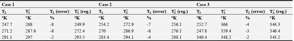
Nevertheless, for sake of comparison between numerical minimum temperature, T and the analytical minimum temperature, T∗, for the tabulated data in Table 4, the results yield that the maximum percentage error, T (error), i.e.,
100 ∗ aT − T∗e T⁄ is 8%. The errors are small with low pressure gradients and they are almost constant for case 3 as the inlet and outlet pressure boundary conditions are fixed. Therefore, to correlate T (error), the results for ΔT ?@(Eq. 7) which have been calculated and inserted in Table 1, Table 2, and Table 3 for variable inlet volume flow rate, Q , beta ratio, β, and pressure ratio, $$ have been modified by non-linear
regression. The fit is achieved to improve the predictive ability of the Equation (7) by adjustment of the three exponents constants by non - linear regression and the results is expressed as:
ΔT ?@ reg. = T ∗ B
' ( . ~C. .•€D
/ " .• E (13)
The modified analytical minimum temperature, T∗ reg. at orifice throat can be obtained by Equation (14).
T∗ reg. = T − ΔT
?@ reg. (14) The regression statistics are as follow, the Multiple R = 0.98, R = 0.96, and the standard error = 4.16.
4. Conclusions and Recommendation
4.1. Conclusions
equation has been examined at a wide range of numerical boundary conditions and showed a good match with the numerical results at lower pressure ratios and a small deviation at higher pressure ratios. Whereas, a maximum absolute error reached 8% between the numerical and analytical minimum temperatures, the equation could be considered appreciably to predict the lowest temperature due to Joule – Thomson effect for accurate selection of orifice downstream piping material within reliable range of operating conditions. Finally, it is verified that the proposed equation, for minimum temperature predictions at orifice throat, not only valid for intermediate and higher pressure boundary conditions but remains so correct at variable beta ratios. It has been found that the prediction of orifice inlet mass flow rate and temperature drop at 6D downstream the orifice via numerical results using k-ε and k-ω turbulence models are aligned will with EN ISO 5761 overall, however it should be noted that exact copying with the derived analytical equation for maximum temperature drops have a different degree of accuracy. This point may lead to a starting point for the final development of EN ISO 5761.
4.2. Recommendation
Because the physical processes occurring during gas expansion (fluid mechanics, heat transfer and thermodynamics) are generally extremely complex, development of a complete description and therefore a model for compressible gas expansion through orifice is effectively impossible. Therefore a modified analytically equation had been obtained by a non-linear multi variable regression need further experimental investigation to cover extreme range of operating conditions. To make special provisions for highest accuracy to cover all operating conditions even in chocked flow, several turbulence models may be used in future studies.
Figure 1. Orifice flow profile layout in piping system.
Figure 2. Meshing for orifice plate with connected upstream and downstream pipes.
Figure 3. Numerical static pressure ratio distributions for fixed outlet pressure, (ƒ = 5.0MPa).
Figure 4. Numerical static temperature ratio distributions for fixed outlet pressure, (ƒ =5.0MPa) and the corresponding analytical minimum temperature ratios calculated by Equation (8) for real methane gas.
Figure 6. Numerical static pressure ratio distributions for fixed inlet pressure, (ƒ =8.3MPa).
Figure 7. Numerical static temperature ratio distributions for fixed outlet pressure, (ƒ =8.3MPa) and the coressponding analytical minimum temperature ratios calculated by Equation (8) for real methane gas.
Figure 8. Numerical static pressure ratio distributions for variable beat ratios (β= 0.3, β= 0.4, and β= 0.5).
Figure 9. Numerical static temperature ratio distributions by k-ω model for (β= 0.3, β= 0.4, and β= 0.5) and the corresponding analytical minimum temperature ratios calculated by Equation (8) for real methane gas.
Table 1. Case 1 results for variable inlet pressure, P1 solved by k-ε model.
Variable inlet pressure, P1 for ( T1 =300°K and β=0.3)
P1 P2 P6D T2 T6D „…†‡
(ISO)
„…†‡ (CFD)
„ˆ†‡ (ISO)
„ˆ†‡ (CFD)
„ˆ‰Š‹ (Eq. 7)
„ˆ‰Š‹
(CFD) qm (ISO) qm
(CFD) qm error
MPa MPa MPa °K °K MPa MPa °K °K °K °K kg/s kg/s %
8.3 4.1 4.7 248 283 3.7 3.5 15.3 16.8 32 52.2 2.219 2.334 -5.2
6.9 4.7 4.9 271 293 1.9 2.0 8.1 6.8 12.4 28.6 1.544 1.658 -7.4
5.5 4.9 5.0 291 298 5.6 5.5 2.3 1.8 3 8.9 0.783 0.879 -12.3
Table 2. Case 2 results for variable outlet pressure, P2 solved by k-ε model.
Variable outlet pressure, P2 for ( T1 =300°K and β=0.3)
P1 P2 P6D T2 T6D „…†‡
(ISO)
„…†‡ (CFD)
„ˆ†‡ (ISO)
„ˆ†‡ (CFD)
„ˆ‰Š‹ (Eq. 7)
„ˆ‰Š‹
(CFD) qm (ISO) qm (CFD) qm error
MPa MPa MPa °K °K MPa MPa °K °K °K °K kg/s kg/s %
8.3 4.4 4.8 254.2 284.8 3.5 3.5 14.3 15.2 27.1 45.8 2.170 2.273 -4.8
8.3 5.5 5.8 270.0 289.6 2.5 2.5 10.3 10.4 13.1 30.0 1.956 2.082 -6.4
8.3 6.6 6.8 283.4 294.1 1.5 1.5 6.1 5.9 5.9 16.6 1.577 1.722 -9.2
Table 3. Case 3 results for variable beta ratio, β solved by k-ω model.
Variable, β ratio (T1 =400°K)
P1 P2 P6D T2 T6D „…†‡
(ISO)
„…†‡ (CFD)
„ˆ†‡ (ISO)
„ˆ†‡ (CFD)
„ˆ‰Š‹ (Eq. 7)
„ˆ‰Š‹ (CFD)
qm
(ISO) qm
(CFD) qm
(error) β
MPa MPa MPa °K °K MPa MPa °K °K °K °K kg/s kg/s % [-]
Variable, β ratio (T1 =400°K)
P1 P2 P6D T2 T6D „…†‡
(ISO)
„…†‡ (CFD)
„ˆ†‡ (ISO)
„ˆ†‡ (CFD)
„ˆ‰Š‹ (Eq. 7)
„ˆ‰Š‹ (CFD)
qm
(ISO) qm
(CFD) qm
(error) β
4.9 2.5 3.0 347.8 395 2.0 2.0 4.9 5.0 40.6 52.2 1.87 1.885 -0.4 0.4
4.9 2.3 3.0 340.4 393 1.9 1.9 4.8 7.0 51.8 59.6 2.99 3.110 -3.7 0.5
Table 4. The comparison between the numerical, Œ and analytical,Œ∗ (by Equations (8) and (14)) minimum temperatures.
Case 1 Case 2 Case 3
ˆ• ˆ•∗ ˆ• (error) ˆ•∗ (reg.) ˆ• ˆ•∗ ˆ• (error) ˆ•∗ (reg.) ˆ• ˆ•∗ ˆ• (error) ˆ•∗ (reg.)
°K °K % °K °K °K % °K °K °K % °K
247.7 268 -8 249.9 254.2 272.9 -7 256.1 252.7 366 -4 344.3
271.2 287.6 -6 272.4 270 286.9 -6 276.1 247.8 359.4 -3 346.4
291.1 297 -2 293.5 283.4 294.1 -4 288.1 340.4 348.2 -2 343.2
Nomenclature
A Pipe cross section area [m ] C Orifice discharge coefficient [-] D Pipe diameter [mm]
d Orifice bore diameter [mm]
Re Reynolds number calculated with respect to D C= Specific heat capacity at constant pressure [Jkg K ] H Specific enthalpy [Jkg ]
i, j, k Grid locations in x, y, z directions k Turbulent kinetic energy [m2/s2] p Mean pressure [kPa]
P^ Static pressure along the pipe centerline [kPa]
P_ Total pressure at the pipe inlet, 2D upstream the orifice [kPa]
4PP^
_9 Pressure ratio due to real gas expansion along pipe centerline [-]
P Inlet static pressure at D distance upstream the orifice [kPa] P Outlet static pressure at ½ D distance downstream the orifice [kPa]
P Fully developed static pressure at 6D distance downstream the orifice [kPa] ∆P Pressure drop, (P − P ) [kPa]
ΔP ?@(CFD) The numerical maximum pressure drop [kPa]
ΔP Pressure drop, (P − P ) [kPa]
ΔP (ISO) Numerical pressure drop, (P − P ) calculated by Equation (3) [kPa]
Q Volume flow rate [m’⁄s] q Mass flow rate [kg/s]
q (CFD) Numerical mass flow rate [kg/s]
q (ISO) Mass flow rate calculated by Equation (1) [kg/s]
R The multiple [-] R Regression factor [-]
T^ Static temperature along the pipe centerline [°K]
T_ Total temperature at the pipe inlet, 2D upstream the orifice [°K]
4TT^
_9 Temperature ratio due to real gas expansion along pipe centerline [-]
T Static temperature at D distance upstream the orifice [°K] T Static temperature at ½ D distance downstream the orifice [°K] '"" (
)* The minimum temperature ratio [-]
T∗ Static temperature at orifice Vena-contracta calculated by Equation (8) [°K]
T Static temperature at 6D distance downstream the orifice [°K] ∆T Temperature drop, (T − T ) [°K]
ΔT ?@(CFD) The numerical maximum temperature drop [°K]
ΔT Temperature drop, (T − T ) [°K]
ΔT (CFD) Numerical temperature drop, (T − T ) [°K]
ΔT ?@ (Eq. 7) Temperature drop,calculated by Equation (7) [°K]
ΔT ?@ reg. Regression temperature drop,calculated by Equation (13) [°K]
τ)Q Stress tensor [Pa]
τ)QU Reynolds stress tensor [Pa] u Velocity [m/s]
u), uQ Velocity tensor [m/s]
u)ˊuQˊ Specific Reynolds shear stress tensor [m /s e
u”• Vena Contracta jetting velocity [m/s]
x), xQ, x– Cartesian coordinates Y Gas expansion coefficient [-]
] Dimensional wall coordinate [-]
x The distance along the orifice and pipe centerlines [mm] Z Compressibility factor [-]
Greek symbols
β (= d/D) Beta ratio [-]
ε Energy Dissipation Rate [m /s’e ω Frequency of dissipation [1/s]
μ!" Joule - Thomson coefficient [°K /Pa]
ρ Fluid density [kg m⁄ ’e
Abbreviations
API American Petroleum Institute
ASME American Standard of Mechanical Engineering ASTM American Standard of Testing and Mechanical CFD Computational Fluid Dynamic
DN Diameter Nominal
EN ISO European National - International Standard Organization SMYS Specified minimum yield stress
Over bars
- Denotes averaged quantity or time-averaged quantity
˜ Denotes dimensional variables
Superscripts
ˊ Denotes fluctuation in turbulent flow, conventionally-averaged variables
˝ Denotes fluctuation in turbulent flow, mass-averaged variables
References
[1] Siba, M., Wanmahmood, W., Zakinuawi, M., Rasani, R., and Nassir, M., 2016, “Flow-Induced Vibration in Pipes: Challengess and Solutions - a Review,” Journal of Engineering Science and Technology, 11 (3) pp. 362 - 382. [2] Ammar, Z., Abdewahid, A., Faiza, S., Abdelkader, M., and Dr.
Barry, J. A., 2016, “Pressure Drop through Orifices for Single-and Two-Phase Vertically Upward Flow-Implication for Metering,” ASME The Journal of Fluids Engineering. [3] Jacob, T., 2015, “Cfd Analysis of Temperature Development
Due to Flow Restriction in Pipeline,” Master Thesis, Department of Mechanical and Structural Engineering and Materials, Faculty of Science and Technology, University of Stavanger
[4] Maric', I., 2005, “The Joule-Thomson Effect in Natural Gas Flow-Rate Measurements,” Flow Measuremnt and Instrumentaion 16 pp. 387-395.
[5] Maric', I., 2007, “A Procedure for the Calculation of the Natural Gas Heat Capacity, the Isentropic Exponent, and the Joule-Thomson Coefficient,” Flow Measuremnt and Instrumentaion 18 pp. 18-26.
[6] Maric', I., and Ivec, I., 2007, “Natural Gas Properties and Flow Computation,” Natural Gas, 29 pp. 501-529.
[7] Lam, C. K. G., and Bremhorst, K. A., 1981, “Modified Form of Model for Prediction Wall Turbulence,” ASME Journal of Fluids of Engineering, 103 pp. 456-460.
[8] BS EN ISO, “Measurement of Fluid Flow by Means of Pressure Differential Devices Inserted in Circular Cross-Section Conduits Running Full — Part 1: General Principles and Requirements,” BS EN ISO 5167-1: 2003.
[9] Martin, A. G., Diego, O. O., Ivan, D. M., Hugo, Y. A., James, C. H., Kenneth, R. H., and Gustavo, A. I., 2013, “A Formulation for Flow Rate of a Fluid Passing through an Orifice Plate from the First Law of Thermodynamics,” Flow Measuremnt and Instrumentaion, 33 pp. 197-201.
[10] Manish, S. S., Jyeshtharaj, B. J., Avtar, S. K., Prasad, C. S. R., and Daya, S. S., 2012, “Analysis of Flow through an Orifice Meter: Cfd Simulation,” Chemical Engineering Science 71, pp. 300-309. [11] Versteeg, H. K., and Malalasekera, M., 2007, “An
Introduction to Computational Fliud,”.
[13] BS-EN-ISO, “Measurement of Fluid Flow by Means of Pressure Differential Devices Inserted in Circular Cross-Section Conduits Running Full — Part 2: Orifice Plates,” BS EN ISO 5167-2: 2003.
[14] BS EN ISO, “Measurement of Fluid Flow by Means of Pressure Differential Devices Inserted in Circular Cross-Section Conduits Running Full — Part 2: Orifice Plates,” BS EN ISO 5167-2: 2003.
[15] Spink, L. K., 1967, “Principles and Practice of Flow Meter
Engineering,” Ninth Edition ed., Foxboro, Massachusetts,
U.S.A.: The Foxboro Company.
[16] Young, D. F., Munson, B. R., and Okiishi, T. H., 2004, “A Brief Introduction to Fluid Mechanics,” Wiley.
[17] ANSYS, “Ansys Fluent Theory Guide,” ([cited Release 15.0 Southpointe November 2013]).
[18] Leutwyler, Z., and Dalton, C., 2004, “A Cfd Study to Analyze the Aerodynamic Torque, Lift, and Drag Forces for a Butterfly Valve in the Mid-Stroke Position,” ASME 2004 Heat Transfer/Fluids Engineering Summer Conference, Paper HT-FED04-56016.