Learning Theory of Randomized Kaczmarz Algorithm
Junhong Lin [email protected]
Ding-Xuan Zhou [email protected]
Department of Mathematics City University of Hong Kong 83 Tat Chee Avenue
Kowloon, Hong Kong, China
Editor:Gabor Lugosi
Abstract
A relaxed randomized Kaczmarz algorithm is investigated in a least squares regression setting by a learning theory approach. When the sampling values are accurate and the regression function (conditional means) is linear, such an algorithm has been well studied in the community of non-uniform sampling. In this paper, we are mainly interested in the different case of either noisy random measurements or a nonlinear regression function. In this case, we show that relaxation is needed. A necessary and sufficient condition on the sequence of relaxation parameters or step sizes for the convergence of the algorithm in expectation is presented. Moreover, polynomial rates of convergence, both in expectation and in probability, are provided explicitly. As a result, the almost sure convergence of the algorithm is proved by applying the Borel-Cantelli Lemma.
Keywords: learning theory, relaxed randomized Kaczmarz algorithm, online learning, space of homogeneous linear functions, almost sure convergence
1. Introduction
The Kaczmarz method is an iterative projection algorithm. It was originally proposed for solving (overdetermined) systems of linear equations, and has been adapted to image reconstruction, signal processing and numerous other applications.
Given a matrix A ∈ Rm×d and a vector b ∈
Rm, the classical Kaczmarz algorithm (Kaczmarz, 1937) approximates a solution of the linear systems Ax = b by an iterative scheme as
xk+1=xk+
bi− hai, xki
kaik2
ai, (1)
where i=k mod m, aT
i is thei-th row of the matrix A, and x1 ∈ Rd is an initial vector. Here h , i is the inner product inRd andk · k the induced norm.
The convergence of the Kaczmarz algorithm (2) is well understood (Kaczmarz, 1937), and its convergence rate depends on the order of rows of A. To avoid this dependence, a randomized Kaczmarz algorithm was considered in (Strohmer and Vershynin, 2009) by setting the probability of a row to be proportional to its norm. It takes the form
xk+1 =xk+
bp(i)− hap(i), xki
kap(i)k2
wherep(i) takes values in {1, . . . , m}with probability kap(i)k2
kAk2 F
withkAk2
F = Pm
i=1
Pd j=1a2ij
being the Frobenius norm square of A. Exponential convergence rate was proved for the expected errorEkxk+1−xk2 of the randomized Kaczmarz algorithm (2) in (Strohmer and Vershynin, 2009). When noise exists in the sample valueb =Ax+ξ with ξ being a noise vector, a bound for the expected error was obtained in (Needell, 2010) and divergence was proved when the variance of ξ is positive. The error bound consists of an exponentially convergent part and a noise-driven term proportional to the noise level maxi ka|ξiik|2.
The randomized Kaczmarz algorithm (2) was generalized in Chen and Powell (2012) to a setting with a sequence of independent random measurement vectors {ϕt∈Rd}t as
xk+1 =xk+
yk− hϕk, xki
kϕkk2
ϕk. (3)
When the measurements have no noise yk = hϕk, xi, almost sure convergence was proved
and quantitative error bounds were provided in (Chen and Powell, 2012).
When the linear system Ax = b is overdetermined (m > d) and has no solution, the Kaczmarz algorithm (2) can be modified by introducing a relaxation parameter ηk >0 in
front of bi−hai,xki
kaik2 ai and the output sequence {xk} converges to the least squares solution arg minx∈RdkAx−bk2 when limk→∞ηk = 0. See, e.g., (Zouzias and Freris, 2013) and
references therein. Setting ψk = kϕ1
kkϕk ∈ S
d−1 and
e
yk = kϕ1
kkyk yields an equivalent form of the scheme (3) as
xk+1=xk+{eyk− hψk, xki}ψk.
This form is similar to those in the literature of online learning for least squares regression and together with the relaxed Kaczmarz method (Zouzias and Freris, 2013) motivates us to consider the following relaxed randomized Kaczmarz algorithm.
Definition 1 With normalized measurement vectors {ψt∈Sd−1}tand sample values {yet∈
R}t, the relaxed randomized Kaczmarz algorithm is defined by
xt+1 =xt+ηt{yet− hψt, xti}ψt, t= 1, . . . , (4)
where x1 ∈Rd is an initial vector and {ηt} is a sequence of relaxation parameters or step
sizes.
The purpose of this paper is to provide learning theory analysis for the relaxed random-ized Kaczmarz algorithm. We shall assume throughout the paper that 0< ηt≤2 for each
t∈Nand that the sequence{zt:= (ψt,yet)}t∈Nis independently drawn according to a Borel
probability measureρ on Z :=Sd−1×R which satisfiesE[|ey|
2]<∞.
Our first goal is to deal with the noisy setting for the randomized Kaczmarz algorithm. When the sampling process is noisy or nonlinear (to be defined below), we show that {xt}t
converges to some x∗ ∈ Rd in expectation if and only if lim
t→∞ηt= 0 and P∞t=1ηt =∞.
Moreover, the rate of convergence in expectation cannot be too fast. It tells us that the relaxation parameter is necessary for the convergence in the noisy setting. When{ηt}ttakes
prove the almost sure convergence. Such results were presented in the case of no noise in (Strohmer and Vershynin, 2009; Chen and Powell, 2012) and are new in the noisy setting.
Our second goal is to give the first almost sure convergence result in online learning for least squares regression when regularization is not needed. Such a result can be found in (Tarr´es and Yao, 2014) when regularization is imposed, while the convergence in expectation without regularization was proved in (Ying and Pontil, 2008). We also present the first consistency result for online learning when the approximation error (to be defined below) does not tend to zero.
2. Main Results
To introduce our learning theory approach to the relaxed randomized Kaczmarz algorithm (4), we decompose the probability measureρonZ =Sd−1×Rinto its marginal distribution
ρX on X := Sd−1 and conditional distributions ρ(·|ψ) at ψ ∈ X. The conditional means define theregression function fρ:X→R as
fρ(ψ) = Z
R
e
ydρ(ye|ψ), ψ∈X. (5)
The hypothesis space for the Kaczmarz algorithm (4) consists of homogeneous linear func-tions
H=
n
fx∈L2ρX : x∈R
do, wheref
x(ψ) :=hx, ψi, ψ∈X. (6)
Definition 2 The sampling process associated with ρ is said to be noise-free if ey =fρ(ψ)
almost surely. Otherwise, it is called noisy. It is said to be linear if fρ ∈ H as a function
in L2ρX. Otherwise, it is called nonlinear.
The main difference between our analysis in this paper and that in the literature (Strohmer and Vershynin, 2009; Needell, 2010; Chen and Powell, 2012) lies in the setting when the sampling process is either noisy or nonlinear. These two situations can be handled simultaneously by means of the least squares generalization error E(f) =RZ(ey−f(ψ))
2dρ, a well developed concept in learning theory. The assumption E[|ye|
2] < ∞ on ρ ensures
fρ∈L2ρX andE(fρ)<∞. The noise-free condition can be stated asE(fρ) = 0.
It is well known that the regression function minimizesE(f) among all the square integral (with respect to ρX) functions f ∈L2ρX, and satisfies
E(f)− E(fρ) =kf−fρk2L2 ρX =
Z
X
(f(ψ)−fρ(ψ))2dρX. (7)
Since the hypothesis spaceH is a finite dimensional subspace ofL2
ρX, the continuous func-tionalE(f) achieves a minimizer
fH= arg min
f∈HE(f). (8)
From (7) we see thatfH is the best approximation offρ in the subspaceH. It is unique as
the orthogonal projection of fρ onto H. It can be written as fH =fx∗ for some x∗ ∈Rd.
The linear condition can be stated as fρ =fH or fρ ∈ H as functions in L2ρX. So we see that the sampling process is noisy or nonlinear if and only if E(fH) > 0. Now we can
state our first main result, to be proved in Section 4, which gives a characterization of the convergence of{xt}t to somex∗ ∈Rd in expectation.
Theorem 3 Define the sequence{xt}t by (4). AssumeE(fH)>0. Then we have the limit
limT→∞Ez1,...,zTkxT+1−x
∗k2 = 0 for some x∗ ∈
Rd if and only if
lim
t→∞ηt= 0 and ∞ X
t=1
ηt=∞. (9)
In this case, we have
∞ X
T=1
q
Ez1,...,zTkxT+1−x
∗k2 =∞. (10)
Compared with the result on exponential convergence in expectation in the linear case without noise (Strohmer and Vershynin, 2009), the somewhat negative result (10) tells us that in the noisy setting the convergence in expectation cannot be as fast asEz1,...,zTkxT+1−
x∗k26=O(T−θ) for anyθ >2. But forθ <1, such learning rates can be achieved by taking
ηt=η1t−θ, as shown in the following second main result, to be proved in Section 4. Theorem 4 Let ηt =η1t−θ for some θ ∈(0,1] and η1 ∈(0,1). Define the sequence {xt}t
by (4). Then for some x∗∈Rd we have
Ez1,...,zTkxT+1−x
∗k2 ≤
(
e
C0T−θ, ifθ <1,
e
C0T−λrη1, ifθ= 1,
(11)
where Ce0 is a constant independent of T ∈ N (given explicitly in the proof ) and λr is the
smallest positive eigenvalue of the covariance matrix CρX of the probability measure ρX
defined by
CρX =EρX[ψψ
T] = Z
X
ψψTdρX. (12)
Our third main result is the following confidence-based estimate for the error which will be proved in Section 5.
Theorem 5 Assume that for some constant M > 0, |ye| ≤ M almost surely. Let θ ∈ [1/2,1], ηt=η1t−θ with 0< η1<min{1,21λr}, and2≤T ∈N. Then for some x∗ ∈Rd and
for any0< δ <1, with confidence at least 1−δ we have
kxT+1−x∗k ≤
(
e
C1T−θ/2 log4δ
2
logT, when θ∈[1/2,1),
e
C1T−λrη1log2δ √
logT , when θ= 1, (13)
where Ce1 is a positive constant independent of T or δ (given explicitly in the proof ).
Theorem 6 Under the assumptions of Theorem 5, we have for any∈(0,1], the following
holds for some x∗ ∈Rd:
(A) When 1/2≤θ <1, limt→∞tθ(1−)/2kxt+1−x∗k= 0 almost surely.
(B) When θ= 1, limt→∞tλrη1(1−)kxt+1−x∗k= 0 almost surely.
Let us demonstrate our setting by two examples without noise considered in the litera-ture. The first example appeared in (Chen and Powell, 2012).
Example 1 If random measurement vectors {ϕt}∞t=1 are independent and nonzero almost
surely, then{ψk = kϕ1kkϕk∈S
d−1} are independent.
The second example is from (Strohmer and Vershynin, 2009).
Example 2 Define the random vector ϕ which is a normalized row of a full rank matrix
A∈Rm×d, with probabilities as
ϕ= aj kajk
with probability kajk
2 kAk2
F
j= 1,· · ·, m.
It was shown in Strohmer and Vershynin (2009) that the smallest eigenvalue of the covari-ance matrix is positive:
λmin(E[ϕϕT])≥ 1 kAk2
FkA−1k2
.
It means r=d and λr ≥ kAk2 1
FkA−1k2
.
The third example is on homoskedastic models (Johnston, 1963).
Example 3 In the literature of homoskedastic models, it is assumed that the sample value
{yt}t satisfies yt = hx∗, ψti+ξt with {ξt}t being independently drawn according to a zero
mean probability measure ξ. This corresponds to the special case when the conditional
distributions ρ(·|ψ) are given by ρ(·|ψ) = fρ(ψ) +ξ. Our setting induced by ρ is more
general and allows heteroskedastic models.
3. Connections to Learning Theory
The relaxed randomized Kaczmarz algorithm defined by (4) may be rewritten as an online learning algorithm with output functions from the hypothesis space (6), and our main results stated in the last section are new even in the online learning literature. To demonstrate this, we denote the tth output function Ft on X induced by the vector xt to be given by
Ft(ψ) =hxt, ψi forψ∈X. Then the iteration relation (4) gives
Ft+1 =Ft+ηt{yet−Ft(ψt)} h·, ψti. (14)
It generates a reproducing kernel Hilbert space (HK,k · kK) by the set of fundamental functions {K(·, x) :x ∈ X } with the inner product hK(·, x), K(·, y)iK = K(x, y). A least
squares regularized online learning algorithm in HK is defined with {(ψt,eyt) ∈ X ×R}t
drawn independently according to a probability measure onZ =X ×R as
Ft+1=Ft−ηt{(Ft(ψt)−eyt)K(·, ψt) +λFt}, t= 1, . . . , (15)
whereλ≥0 is a regularization parameter. The consistency of the online learning algorithm (15) is well understood when the approximation errorD(λ) tends to zero asλ→0.
Definition 7 The approximation error (or regularization error) of the pair(ρ, K)is defined for λ >0 as
D(λ) = inf
f∈HK
E(f)− E(fρ) +λkfk2K = inf f∈HK
n
kf −fρk2L2
ρX +λkfk 2
K o
. (16)
When λ > 0 (with regularization) and limλ→0D(λ) = 0, the error kFT+1−fρk2L2 ρX in expectation and in confidence was bounded in (Smale and Yao, 2005; Ying and Zhou, 2006; Smale and Zhou, 2009; Tarr´es and Yao, 2014) by means of the decay of D(λ) andT. The error analysis was done in Ying and Pontil (2008) without regularization (λ= 0) but under the approximation error condition limλ→0D(λ) = 0. The error kFT+1−fρk2K with the
HK-metric was also analyzed whenfρ∈ HK.
If we take the kernel to be the linear one: K(x, y) =hx, yi with X =Rd, and assume that the marginal distributionρX is supported onX =Sd−1, thenψt∈Sd−1 almost surely. Set λ= 0, we see that the relaxed randomized Kaczmarz algorithm expressed in the form (14) is the least squares online learning algorithm (15) without regularization. So the error analysis from Ying and Pontil (2008) applies, but the condition limλ→0D(λ) = 0 is required for the consistency inL2ρX and even stronger conditions (stronger thanfρ∈ HK) are needed
for the consistency in the HK-metric.
Notice that for the linear kernel,kxk=kh·, xikK. So the error analysis carried out in this
paper provides bounds for the errorkFT+1−fHkK without the condition limλ→0D(λ) = 0. Such results cannot be found in the literature of online learning. It leads to the problem of carrying our similar error analysis for more general online learning algorithms associated with more general kernels. Moreover, the best convergence rate in expectation of the general kernel-based least squares online learning algorithm is O(T−1/2) in the literature (Smale and Yao, 2005; Ying and Zhou, 2006; Smale and Zhou, 2009; Tarr´es and Yao, 2014; Hu et al., 2015). Theorem 4 demonstrates that the special online learning algorithm (4) has convergence rates of typeO(T−(1−)) for any >0 and even of typeO(T−1logT) shown in Theorem 8 below, which is a great improvement.
Note that there is a gap between the negative result (10) and the positive one (11), which leads to the natural question whether learning rates of typeEz1,...,zTkxT+1−x
∗k2=O(T−θ)
Theorem 8 Let λr be as in Theorem 4 and ηt = λr(t1+t0) for some t0 ∈ N such that
t0λr≥1. Define the sequence {xt}t by (4). Then for some x∗ ∈Rd, we have
Ez1,···,zTkxT+1−x
∗k2 ≤
e
C3(T +t0)−1logT,
where Ce3 is a constant independent of T ∈N(given explicitly in the proof ).
4. Convergence in Expectation
In this section we prove our main results on convergence in expectation. To this end, we need some preliminary analysis.
Recall the functionfHdefined by (8). It equalsfx∗ for somex∗ ∈Rd. As the orthogonal
projection offρonto the finite dimensional subspaceHin the Hilbert spaceL2ρX, it satisfies hfρ−fx∗, fxiL2
ρX =
Z
X
(fρ(ψ)− hx∗, ψi)hx, ψidρX(ψ) = 0, ∀x∈Rd. (17)
The vector x∗ is not necessarily unique. To see this, we use the covariance matrix
CρX of the measureρX defined by (12) and denote its eigenvalues to be λ1 ≥. . . ≥λr >
λr+1 = . . . = λd = 0 where r ∈ {1, . . . , d} is the rank of CρX. Denote the eigenspace of CρX associated with the eigenvalue 0 as V0 and the orthogonal projection onto V0 as
P0. Then any vector x∗+v from the set x∗ +V0 is also a minimizer of E(fx) in Rd, but
fx∗+v=fx∗ =fH as functions in the space L2 ρX.
The following lemma about the residual vectors {rt=xt−x∗}t is a crucial step in our
analysis in this section.
Lemma 9 Define the sequence {xt}t by (4). Let x∗ ∈Rd be such that fx∗ = fH. Denote
rt=xt−x∗. Then there holds
Ezt[krt+1k 2] =kr
tk2+ (−2ηt+ηt2)kfrtk 2
L2 ρX +η
2
tE(fH), ∀ t∈N. (18)
Proof Subtractx∗ from both sides of (4) and take inner products. We see from kψtk= 1
that
krt+1k2 =krtk2+ 2ηt{yet− hψt, xti} hψt, rti+η
2
t{yet− hψt, xti}
2. (19)
Sincextdoes not depend onzt, taking expectation with respect tozt, we see fromE[yet|ψt] =
fρ(ψt) andEzt{eyt− hψt, xti}
2 =E(f
xt) that
Ezt[krt+1k 2] =kr
tk2+ 2ηtEψt[{fρ(ψt)− hψt, xti} hψt, rti] +η 2
tE(fxt). By (17), we know that the middle term above equals
2ηtEψt[{hψt, x
∗i − h
ψt, xti} hψt, rti] = 2ηtEψt[{hψt,−rti} hψt, rti] =−2ηtkfrtk 2
L2 ρX.
Since fx∗ is the orthogonal projection of fρ onto H, there holds E(fx
t) = E(fρ) +kfρ−
fx∗k2 L2
ρX +kfx
∗−fx
tk 2
L2
ρX =E(fH) +kfrtk 2
L2
We are in a position to prove our first main result.
Proof of Theorem 3 Necessity. We first analyze the first two terms of the right hand side of the identity (18) in Lemma 9. Since 0 < ηt ≤ 2, we have −2ηt+ηt2 < 0. Observe
from the Schwarz inequality that |frt(ψ)|
2 = |hr
t, ψi|2 ≤ krtk2kψk2 = krtk2 and thereby
kfrtk 2
L2
ρX ≤ krtk
2. It follows that krtk2+ (−2ηt+η2t)kfrtk
2
L2
ρX ≥ krtk
2+ (−2η
t+ηt2)krtk2 = (1−ηt)2krtk2.
This together with (18) implies
Ezt[krt+1k
2]≥(1−η
t)2krtk2+η2tE(fH). (20)
Then we can proceed with proving the necessity. If limT→∞Ez1,...,zTkxT+1−x
∗k2 = 0 for some x∗ ∈ Rd and E(f
H) > 0, we know from (20) that limT→∞ηT = 0. It ensures the
existence of some integer t0 ≥2 such that ηt≤ 13 for anyt≥t0. Since 1−η≥exp{−2η}
for 0< η ≤ 13, we know that for any t≥t0, (1−ηt)2 ≥exp{−4ηt}. Combining this with
(20) yields
Ez1,...,zTkxT+1−x
∗k2≥ΠT
t=t0exp{−4ηt}Ez1,...,zt0−1krt0k 2. But (20) also tells us thatEz1,...,zt0−1krt0k
2 ≥η2
t0−1E(fH)>0. So
Ez1,...,zTkxT+1−x
∗k2 ≥exp
(
−4
T X
t=t0
ηt )
ηt20−1E(fH).
Since limT→∞Ez1,...,zTkxT+1 −x
∗k2 = 0, we must have P∞
t=1ηt = ∞. This proves the
necessity.
Sufficiency. Recall that V0 is the eigenspace of the covariance matrix CρX associated
with the eigenvalue 0 andP0 is the orthogonal projection ontoV0. Thenψt is orthogonal to
V0 almost surely for each t. It follows that P0(xt+1) =P0(xt) and thereby P0(xt) =P0(x1) for eacht. Take the vectorx∗to be the minimizer ofE(fx) inRdsuch thatP0(x∗) =P0(x1). With this choice,rtis orthogonal toV0for eacht, and belongs to the orthogonal complement
V0⊥. Note that the eigenvalues of CρX restricted to the subspace V
⊥
0 is at least λr >0. So
we have
kfrtk 2
L2 ρX =
Z
X
|hψ, rti|2dρX = Z
X
rtTψψTrtdρX =rtTCρXrt (21)
and kfrtk 2
L2
ρX ≥λrkrtk
2.The condition lim
t→∞ηt= 0 ensures the existence of somet1 ∈N such thatηt≤1 for anyt≥t1.Thus, we see from (18) in Lemma 9 that fort≥t1,
Ezt[krt+1k 2]≤ kr
tk2−ηtkfrtk 2
L2 ρX +η
2
tE(fH)≤(1−ηtλr)krtk2+ηt2E(fH).
Applying this inequality iteratively for t=T,· · ·t1 yields
Ez1,...,zT[krT+1k 2]≤
Ez1,...,zt1−1[krt1k 2]
T Y
t=t1
(1−ηtλr) +E(fH) T X
t=t1
η2t
T Y
k=t+1
where we denoteQTk=t+1(1−ηkλr) = 1 for t=T. By the condition P∞t=1ηt=∞,one has T
Y
t=t1
(1−ηtλr)≤exp (
−λr T X
t=t1
ηt )
→0 as T → ∞.
Thus for anyε >0,there existst2 =t2(ε)∈N such that for anyT ≥t2,
Ez1,...,zt1−1[krt1k 2]
T Y
t=t1
(1−ηtλr)≤ε.
To deal with the other term of the bound (22) forkrT+1k2, we use the assumption limt→∞ηt=
0,and find some integer t(ε)≥t1 such that ηt≤λrε for anyt≥t(ε).Write T
X
t=t1
ηt2
T Y
k=t+1
(1−ηkλr) = t(ε)
X
t=t1
ηt2
T Y
k=t+1
(1−ηkλr) + T X
t=t(ε)+1
ηt2
T Y
k=t+1
(1−ηkλr). (23)
The second term of (23) can be bounded as
T X
t=t(ε)+1
η2t
T Y
k=t+1
(1−ηkλr) = ε T X
t=t(ε)+1
ηtλr T Y
k=t+1
(1−ηkλr)
= ε
T X
t=t(ε)+1
(1−(1−ηtλr)) T Y
k=t+1
(1−ηkλr)
= ε
1− T Y
k=t(ε)+1
(1−ηkλr)
≤ε.
To bound the first term of (23), we apply the conditionP∞t=1ηt=∞ again and find some
integert3 =t3(ε)> t(ε) such thatPtk3=t(ε)+1ηk ≥ λ1r logt(εε). Hence T
X
k=t(ε)+1
ηk ≥ t3
X
k=t(ε)+1
ηk≥
1
λr
logt(ε)
ε , ∀ T ≥t3.
It thus follows that for each t∈ {t1, . . . , t(ε)},
T Y
k=t+1
(1−ηkλr)≤exp (
−λr T X
k=t+1
ηk ) ≤exp
−λr T X
k=t(ε)+1
ηk
≤ ε
t(ε).
Combining with the fact ηt ≤ 1 for each t≥ t1, we see that the first term of (23) can be bounded as
t(ε)
X
t=t1
ηt2
T Y
k=t+1
(1−ηkλr)≤
ε t(ε)
t(ε)
X
t=t1
From the above analysis, we know that when T ≥max{t1, t(ε), t2, t3}, Ez1,...,zT[krT+1k
2]≤ε+ 2E(f
H)ε.
This proves the convergence limT→∞Ez1,...,zTkxT+1−x
∗k2 = 0 for some x∗ ∈
Rd and the sufficiency is verified.
From the bound (20), we also see that
Ez1,...,zTkxT+1−x
∗k2 ≥η2
TE(fH), ∀T ∈N. This implies that
∞ X
T=1
q
Ez1,...,zTkxT+1−x
∗k2≥p
E(fH) ∞ X
T=1
ηT =∞.
The proof of Theorem 3 is complete.
In the proof of our second main result, we need some elementary inequalities.
Lemma 10 (a) For ν, a >0, there holds
exp{−νx} ≤ a
νe
a
x−a, ∀x >0. (24)
(b) Let ν >0 and q2 ≥0. If 0< q1 <1, then for any t∈N, we have
t−1
X
i=1
i−q2exp
−ν
t X
j=i+1
j−q1
≤ 2
q1+q2
ν +
1 +q2
ν(1−2q1−1)e
11+−qq2
1
!
tq1−q2. (25)
For q1= 1, we have
t−1
X
i=1
i−q2exp
−ν
t X
j=i+1
j−1
≤
(
2q2
|ν−q2+1|t
−min{ν,q2−1}, if ν 6=q 2−1, 2q2t−νlogt, if ν =q
2−1.
(26)
(c) For any t < T ∈N and θ∈(0,1], there holds
T X
k=t+1
k−θ ≥
1
1−θ[(T+ 1)1−θ−(t+ 1)1−θ], if θ <1,
log(T + 1)−log(t+ 1), if θ= 1. (27)
(d) For θ∈(0,1], µ >0, andT ∈N,there holds
exp
(
−µ
T X
t=1
t−θ
)
≤
expn1−θµ o µθe θ 1−θ
T−θ, ifθ <1,
T−µ, ifθ= 1.
(28)
Part (c) can be proved by noting that
T X
k=t+1
k−θ≥
T X
k=t+1
Z k+1
k
x−θdx=
Z T+1
t+1
x−θdx.
For part (d), we use the inequality (27) in part (c) to derive
exp ( −µ T X t=1 t−θ ) ≤ ( exp n µ 1−θ o exp n
−1−θµ T1−θ
o
, ifθ <1,
T−µ, ifθ= 1.
Forθ∈(0,1), by applying (24) with ν = 1−θµ ,x=T1−θ and a= 1−θθ , we get
exp
− µ 1−θT
1−θ ≤ θ µe
1−θθ
T−θ.
This proves the result.
We can now prove our second main result. This is done by following the estimate (22) in the proof of Theorem 3.
Proof of Theorem 4 Since η1 <1, we haveηt <1 for all t∈N. Therefore, we can take
t1 = 1 in (22) and obtain
Ez1,...,zT[krT+1k
2] ≤ kr 1k2
T Y
t=1
(1−ηtλr) +E(fH) T X
t=1
η2t
T Y
k=t+1
(1−ηkλr)
≤ kr1k2exp
(
−λrη1
T X
t=1
t−θ
)
+E(fH)η12 T X
t=1
t−2θexp
(
−λrη1
T X
k=t+1
k−θ
)
. (29)
Applying part (d) withµ=λrη1 of Lemma 10, we know that the first term of (29) can be bounded as
kr1k2exp
(
−λrη1
T X t=1 t−θ ) ≤
kr1k2exp
n λrη1
1−θ o
θ λrη1e
1−θθ
T−θ, ifθ <1,
kr1k2T−λrη1, ifθ= 1.
Applying part (b) of Lemma 10 with q1 =θ, q2 = 2θ, ν =λrη1, and noting that λrη1 <1 by η1∈(0,1) and λr ∈(0,1], we know that the second term of (29) can be bounded by
E(fH)η12
1 +λ23θ rη1 +
1+2θ λrη1(1−2θ−1)e
1+21−θθ
T−θ, ifθ <1,
E(fH)η12
1 +1−λ4 rη1
Thus, we get our desired result with Ce0 given by
e
C0 =
kr1k2exp
n λrη1
1−θ o
θ λrη1e
1−θθ
+E(fH)η12
λrη1+23θ
λrη1 +
1+2θ λrη1(1−2θ−1)e
1+21−θθ
, ifθ <1,
kr1k2+E(fH)η12
1 +1−λ4 rη1
, ifθ= 1.
This completes the proof of Theorem 4.
Remark 11 From the proof of Theorem 4, we see that ifE(fH) = 0,then for somex∗ ∈Rd,
we have
Ez1,...,zT[krT+1k 2]≤ kr
1k2
T Y
t=1
(1−ηtλr).
The above argument actually can be used to prove Theorem 8.
Proof of Theorem 8 Since η1≤1,we haveηt≤1 for allt∈N.Thus, we can taket1 = 1 in (22) and obtain
Ez1,...,zT[krT+1k
2] ≤ kr 1k2
T Y
t=1
(1−ηtλr) +E(fH) T X
t=1
η2t
T Y
k=t+1
(1−ηkλr)
= kr1k2
T Y
t=1
1− 1
t+t0
+E(fH)
λ2 r T X t=1 1 (t+t0)2
T Y
k=t+1
1− 1
k+t0
.
We note that
T Y
k=t+1
1− 1
k+t0
=
T Y
k=t+1
k+t0−1
k+t0
= t+t0
T +t0
.
It thus follows that
Ez1,...,zT[krT+1k 2]≤ kr
1k2
t0
T +t0
+E(fH)
λ2
r
1
T+t0
T X
t=1 1
t+t0
.
WithPTt=1 t+1t
0 ≤log
T+t0
t0+1 ≤logT, we get the desired result withCe3 given by
e
C3=t0kr1k2+ E(fH)
λ2
r
.
5. Confidence-Based Estimates for Convergence
In this section, we prove our third main result, Theorem 5. Recall thatV0is the eigenspace of the covariance matrixCρX associated with the eigenvalue 0. We choosex
∗as in the proof of
the sufficiency part of Theorem 3. With this choice,rtbelongs to the orthogonal complement
V0⊥ almost surely. Our error analysis is based on the following error decomposition. 5.1 Error Decomposition
Fort∈N, set the operator Πtk=Qtj=k(I−ηjCρX) onR
dfork≤tand Πt
t+1=I.Subtracting
x∗ from both sides of (4), we have
rk+1= (I−ηkCρX)rk+ηkχk, (30) where
χk= (˜yk− hψk, x∗i)ψk+ (CρX−ψkψ
T k)rk.
Applying this relationship iteratively for k=t,· · ·,1, we get
rt+1 = Πt1r1+
t X
k=1
ηkΠtk+1χk.
Thus
krt+1k ≤
Πt1r1
+
t X
k=1
ηkΠtk+1χk
. (31)
The first term of the bound (31) is caused by the initial error, which is deterministic and will be estimated in subsection 5.2. The second term is the sample error depending on the sample. Since rk is independent of zk, byE[˜yk|ψk] =fρ(ψk) and (17),
E[χk|z1, . . . , zk−1] =
Z
X
(fρ(ψ)− hx∗, ψi)ψ+ (CρX −ψψ
T)r
kdρX(ψ) = 0.
It tells us that{ωk:=ηkΠtk+1χk}kis a martingale difference sequence. The idea of analyzing
the sample error by properties of martingale difference sequences can be found in the recent work in (Tarr´es and Yao, 2014) to which details about martingale difference sequences are referred. In particular, we can apply the following Pinelis-Bernstein inequality from (Tarr´es and Yao, 2014) (derived from (Pinelis, 1994, Theorem 3.4)) to estimate the sample error.
Lemma 12 Let{ωk}k be a martingale difference sequence in a Hilbert space. Suppose that
almost surely kωkk ≤ B and Ptk=1E[kωkk2|ω1, . . . , ωk−1]≤ L2t. Then for any 0 < δ < 1,
the following holds with probability at least 1−δ,
sup 1≤j≤t
j X
k=1
ωk
≤2
B
3 +Lt
log2
δ.
5.2 Initial Error
Lemma 13 Let ηk=η1k−θ withθ∈(0,1] andη1∈(0,1).Then kΠt1r1k ≤
C0t−θ, when θ <1,
C0t−λrη1, when θ= 1,
where
C0 =
kr1kexp
n λrη1
1−θ o
θ λrη1e
1−θθ
, when θ <1,
kr1k, when θ= 1.
Proof By our choice of x∗, we know thatr1 belongs to the subspaceV0⊥. Thus, we have kΠt1r1k ≤ kΠt1|V0⊥kkr1k.
Here Πt1|V⊥
0 denotes the restriction of the self adjoint operator Π
t
1 ontoV0⊥. Since{λl:l=
1,2,· · ·, r}are the eigenvalues of CρX restricted to V
⊥
0 ,λ1 ≤1 andη1<1, we have kΠt1|V⊥
0 k= sup 1≤l≤r
t Y
k=1
(1−ηkλl)≤ t Y
k=1
(1−η1λrk−θ)≤exp (
−λrη1
t X
k=1
k−θ
)
.
Applying part (d) of Lemma 10, we get our desired result.
5.3 Bounding the Residual Sequence
To bound ωk=ηkΠkt+1χk, we start with a rough bound forkrtk.
Lemma 14 Assume that for some constant M >0, |ey| ≤M almost surely. Let θ∈[0,1]
and ηt=η1t−θ withη1∈(0,1). Then for any t∈N, we have almost surely
krtk ≤ (
C1t 1−θ
2 , whenθ∈[0,1),
C1
p
log(et), whenθ= 1, (32)
where C1 is a constant independent of t given by
C1 =
( q
kr1k2+η1(M+kx∗k)2
1−θ , when θ∈[0,1), p
kr1k2+η1(M+kx∗k)2, when θ= 1. Proof Rewrite (19) withxt=x∗+rt as
krt+1k2 = krtk2+ 2ηt(˜yt− hψt, x∗i − hψt, rti)hψt, rti
+ηt2(˜yt− hψt, x∗i − hψt, rti)2
whereF :R→Ris a quadratic function given by
F(µ) =Fηt,y˜t,ψt,x∗(µ) =ηt(ηt−2)µ2+ 2ηt(1−ηt)(˜yt− hψt, x∗i)µ+ηt2(˜yt− hψt, x∗i)2.
Note thatηt(ηt−2)≤0 by 0< ηt≤η1 ≤1.A simple calculation shows that max
x∈RF(x) =−
ηt2(1−ηt)2(˜yt− hψt, x∗i)2
ηt(ηt−2)
+η2t(˜yt− hψt, x∗i)2 =
ηt(˜yt− hψt, x∗i)2
2−ηt
.
Since |˜yt| ≤M almost surely and kψtk= 1,
|˜yt− hψt, x∗i| ≤ |y˜t|+kψtkkx∗k ≤M+kx∗k.
Thus,
krt+1k2≤ krtk2+
ηt(˜yt− hψt, x∗i)2
2−ηt
≤ krtk2+ηt(M +kx∗k)2.
Using this relationship iteratively yields
krt+1k2≤ kr1k2+
t X
k=1
ηk(M+kx∗k)2=kr1k2+η1(M +kx∗k)2
t X
k=1
k−θ.
Since that
t X
k=1
k−θ≤1 +
t X
k=2
Z k
k−1
x−θdx=
( t1−θ−θ
1−θ , when θ∈[0,1),
log(et), when θ= 1,
we get
krtk2 ≤ (
kr1k2+η1(M+kx∗k)2 1−θ t1
−θ, whenθ∈[0,1),
(kr1k2+η1(M+kx∗k)2) log(et), whenθ= 1, which leads to the desired result.
5.4 Estimating Conditional Variance and Upper Bound
In this subsection, we give bounds for the two termsPtk=1η2kE[kΠtk+1χkk2|z1, . . . , zk−1] and sup1≤k≤tkηkΠtk+1χkkrequired in applying the Pinelis-Bernstein inequality.
Lemma 15 Let ηk=η1k−θ withθ∈(0,1] andη1∈(0,1).Then almost surely we have
t X
k=1
η2kE[kΠtk+1χkk2|z1, . . . , zk−1]
≤
t X
k=1
η21k−2θexp
−2η1λr t X
j=k+1
j−θ
E(fH) +krkk22
.
Proof Recall that bothψk andrk belong toV0⊥almost surely for eachk∈N. As a result,
χk also belongs to V0⊥ almost surely for each k. Hence
t X
k=1
ηk2E[kΠtk+1χkk2|z1, . . . , zk−1]≤
t X
k=1
ηk2kΠt k+1|V⊥
0 k 2
E[kχkk2|z1, . . . , zk−1]. Since η1<1 andλ1≤1, we have
Π
t k+1|V⊥
0 = sup 1≤l≤r t Y
j=k+1
(1−ηjλl)≤ t Y
j=k+1
(1−ηjλr)
≤ exp
−λr t X
j=k+1
ηj = exp
−λrη1
t X
j=k+1
j−θ . (34) Thus, t X k=1
η2kE[kΠtk+1χkk2|z1, . . . , zk−1]
≤
t X
k=1
ηk2exp
−2λrη1
t X
j=k+1
j−θ
E[kχkk2|z1, . . . , zk−1].
(35)
Since rk does not depend on zk, we see fromkψkk= 1,E[˜yk|ψk] =fρ(ψk) and (17) that
Ezk[h(˜yk− hψk, x
∗i)ψ
k,(CρX −ψkψ
T k)rki]
=Ezk[(˜yk− hψk, x
∗i)hψ
k, CρXrki]−Ezk[(˜yk− hψk, x
∗i)hψ
k, rkikψkk2]
=Eψk[(fρ(ψk)− hψk, x
∗i)hψ
k, CρXrki]−Eψk[(fρ(ψk)− hψk, x
∗i)hψ
k, rki] = 0.
It thus follows that
E[kχkk2|z1, . . . , zk−1] =Ezk[kχkk 2] =Ezk[(˜yk− hψk, x
∗i)2] +
Ezk[k(CρX −ψkψ
T k)rkk2]
=E(fH) +Ezkh(CρX−C 2
ρX)rk, rki ≤ E(fH) +krkk22.
Putting the above bound into (35), we get the desire result.
Lemma 16 Assume that for some constant M >0, |ey| ≤M almost surely. Let θ∈[0,1]
and ηt=η1t−θ withη1∈(0,1). Then for any t∈N, we have almost surely
sup 1≤k≤t
kηkΠtk+1χkk ≤
C2t−θmax
sup1≤k≤tkrkk, 1 , when θ <1,
C2t−λrη1max
sup1≤k≤tkrkk, 1 , when θ= 1,
(36)
where C2 is a constant given by
C2 =
η1(M+kx∗k+ 2)
2θ+eλ θ rη1(1−2θ−1)
1−θθ
Proof Let k∈ {1, . . . , t}.From the definition ofχk, we have
kχkk ≤(|˜yk|+kψkkkx∗k)kψkk+kCρX −ψkψ
T kkkrkk.
But |˜yk| ≤M,kψkk= 1 and kCρXk ≤1.So we have
kχkk ≤M+kx∗k+ 2krkk ≤(M+kx∗k+ 2) max{krkk,1}.
This together with (34) and the fact that χk belongs to V0⊥ implies kηkΠtk+1χkk ≤ η1k−θkΠtk+1|V0⊥kkχkk
≤ η1(M+kx∗k+ 2)k−θkΠtk+1|V⊥
0 kmax{krkk,1}
≤ η1(M+kx∗k+ 2)k−θexp
−λrη1
t X
j=k+1
j−θ
max{krkk,1}.
What is left is to estimate
Ik:=k−θexp
−λrη1
t X
j=k+1
j−θ
.
Forθ∈[1/2,1),applying part (c) of Lemma 10 gives
Ik≤k−θexp
−λrη1
1−θ[(t+ 1)
1−θ−
(k+ 1)1−θ]
.
Ifk≥t/2,then k−θ≤2θt−θ and thus
Ik≤2θt−θ.
If 1≤k < t/2,then we havek+1≤(t+1)/2 and (t+1)1−θ−(k+1)1−θ ≥(1−2θ−1)(t+1)1−θ.
It follows that
Ik ≤exp
−λrη1(1−2
θ−1) 1−θ t
1−θ
.
Applying part (a) of Lemma 10 with x=t1−θ,ν = λrη1(1−2θ−1)
1−θ and a= 1−θθ , we get
Ik ≤
θ
eλrη1(1−2θ−1)
1−θθ
t−θ.
Forθ= 1, by part (c) of Lemma 10, with λrη1 <1, we have
Ik≤k−1
t+ 1
k+ 1
−λrη1 =
t t+ 1·
k+ 1
k
λrη1
5.5 Preliminary Error Analysis
Based on the above estimates, we can apply Lemma 12 to obtain an error bound.
Proposition 17 Under the assumptions of Theorem 5, for some x∗ ∈ Rd and for any
0< δ <1 and fixedt∈N, with confidence at least 1−δ, we have
kxt+1−x∗k ≤
(
e
C2t 1
2−θlog2
δ, whenθ∈[
1 3,1),
e
C2t−λrη1
p
log(et) log2δ, whenθ= 1, (37)
where Ce2 is a positive constant independent of t or δ (given explicitly in the proof ).
Proof To apply the Pinelis-Bernstein inequality to estimate kPt
k=1ηkΠtk+1χkk, we need
bounds B andLt.
By Lemmas 14 and 16, we have
sup 1≤k≤t
kηkΠtk+1χkk ≤ (
C2(C1+ 1)t 1−3θ
2 , whenθ <1,
C2(C1+ 1)t−λrη1
p
log(et), whenθ= 1. (38)
By Lemmas 15 and 14, we get
t X
k=1
η2kE[kΠtk+1χkk2|z1, . . . , zk−1]
≤
C3Ptk=1k−(3θ−1)exp
n
−2λrη1Ptj=k+1j−θ
o
, when θ∈[13,1), C3log(et)Ptk=1k−2exp
n
−2λrη1Ptj=k+1j−1
o
, when θ= 1,
where
C3= (E(fH) +C12)η21.
Applying part (b) of Lemma 10 with ν = 2λrη1 <1, q1 =θ and q2 = 3θ−1, we have for
θ <1,
t X
k=1
k−(3θ−1)exp
−2λrη1
t X
j=k+1
j−θ
≤ 2 4θ−1 2λrη1
+
3θ
2λrη1e(1−2θ−1)
13−θθ!
t1−2θ+t1−3θ,
and for θ= 1,
t X
k=1
k−2exp
−2λrη1
t X
j=k+1
j−1
≤ 4 1−2λrη1
t−2λrη1 +t−2.
Therefore, we get
t X
k=1
ηk2E[kΠtk+1χkk2|z1, . . . , zk−1]≤
C4t1−2θ, when θ∈[13,1),
C4t−2λrη1log(et), when θ= 1,
with
C4=
C3
24θ−1 2λrη1 +
3θ
2λrη1e(1−2θ−1)
13−θθ
+ 1
, when θ∈[13,1), C315−−22λλrrηη11, when θ= 1.
Applying Lemma 12 to the martingale difference sequence {ωk :=ηkΠtk+1χk}k with B
and Lt given by (38) and (39) respectively, we know that with probability at least 1−δ,
sup 1≤j≤t
j X
k=1
ηkΠtk+1χk
≤
(
C5t 1−2θ
2 log2
δ, when θ∈[
1 3,1),
C5t−λrη1
p
log(et) log2δ, when θ= 1,
where
C5= 2
C2(C1+ 1)/3 +
p
C4
.
Putting this bound into (31) with treplaced by j, and then applying Lemma 13 to bound the initial error, we get the desired result withCe2=C0+C5 from Lemma 12.
In the above procedure, we have used a rough bound (32) for krtk. This rough bound
tends to∞ astbecomes large. In contrast, the bound provided in Proposition 17 tends to 0 (whenθ∈(1/2,1]) and is much better. But this bound holds with confidence. We shall use this refined bound to improve our estimates in the following subsection.
5.6 Improved Error Analysis
In this subsection, we prove our third main result by improving the preliminary confidence-based error bound in Proposition 17.
Proof of Theorem 5 When θ= 1,our desired bound follows from (37) with Ce1 = 2Ce2.
It remains to prove the case θ ∈ [1/2,1). Let T ∈ N. Applying Proposition 17 with
t= 1,· · · , T, and taking the union event followed by rescaling, we know that there exists a subsetZδT of ZT with measure at least 1−δ such that
krtk ≤C6log 2
δlogT, ∀t= 1, . . . , T + 1, (z1, . . . , zT)∈Z
T
δ, (40)
whereC6 = 2Ce2+kr1k.
Now we turn to the essential part of the proof. Define another martingale difference sequence {ωek}k by multiplying the one in the proof of Proposition 17 by a characteristic
function1{kr
kk≤C6log2δlogT} as
e
ωk=ηkΠTk+1χk1{krkk≤C6log2δlogT}.
From (36) and the multiplication with the characteristic function 1{kr
kk≤C6log2δlogT}, we have
sup 1≤k≤T
kωekk ≤C2C6log
2
δ
Notice that the characteristic function 1{kr
kk≤C6log2δlogT} is independent of zk. Also, from the proof of Lemma 15, we know that for eachk∈ {1, . . . , T},
E[kΠtk+1χkk2|z1, . . . , zk−1]≤exp
−λrη1
t X
j=k+1
j−θ
E(fH) +krkk22
.
It follows by setting C7= (E(fH) +C62)η21 that
T X
k=1 E
h
keωkk2|z1, . . . , zk−1
i
≤C7
log2
δ logT
2 T X
k=1
k−2θexp
−2λrη1
T X
j=k+1
j−θ
.
Applying part (b) of Lemma 10 yields
T X
k=1 E
h
keωkk2|z1, . . . , zk−1
i
≤C7
log2
δ logT
2
23θ
2λrη1 +
1 + 2θ
2λrη1e(1−2θ−1) 1+21−θθ
+ 1
!
T−θ.
Using this bound as LT and (41) as the bound B in Lemma 12, we know that there exists
another subset ˜ZδT ofZT with measure at least 1−δ such that for every (z1, . . . , zT)∈Z˜δT,
there holds T X k=1 e ωk
≤C8T
−θ 2 log2 δ 2 logT, where
C8=
2C2C6 3 + 2
p
C7
23θ+ 2λrη1 2λrη1
+
1 + 2θ
2λrη1e(1−2θ−1)
1+21−θθ!
1 2
.
This together with (40) tells us that for every (z1, . . . , zT)∈ZδT ∩Z˜δT, there holds T X k=1
ηkΠTk+1χk
≤C8T
−θ 2 log2 δ 2
logT. (42)
The subsetZδT ∩Z˜δT has measure at least 1−2δ. Therefore, we can put (42) into (31), and apply Lemma 13 to bound the initial error, which proves Theorem 5 for the caseθ∈[1/2,1) after scalingδ toδ/2 and setting the constantCe1 =C0+C8.
6. Almost Sure Convergence
In this section, we prove the almost sure convergence of the randomized Kaczmarz algorithm. Recall that the almost sure convergence of a sequence of random variables {Xn} towards
X means that
P
lim
n→∞Xn=X
or equivalently,
lim
n→∞P
sup
k≥n
|Xk−X|> ε
= 0 for any ε >0.
The Borel-Cantelli Lemma (see e.g. (Klenke, 2010)) asserts for a sequence (En)n of
events that if the sum of the probabilities is finite P∞n=1P(En) <∞, then the probability
that infinitely many of them occur is 0, that is,P(lim supn→∞En) =P(∩n∞=1∪∞k=nEn) = 0.
The following lemma is an easy consequence of the Borel-Cantelli Lemma. We give the proof for completeness.
Lemma 18 Let {Xn} be a sequence of events in some probability space and {εn} be a
sequence of positive numbers satisfyinglimn→∞εn= 0.If
∞ X
n=1
P(|Xn−X|> εn)<∞,
thenXn converges to X almost surely.
Proof Since limn→∞εn= 0,for anyε >0,there exists somen∈Nsuch that for allk≥n,
εk< ε. Thus,
P
sup
k≥n
|Xk−X|> ε
≤P [
k≥n
(|Xk−X|> εk)
≤X
k≥n
P
|Xk−X|> εk
.
Letting n→ ∞, one gets P supk≥n|Xk−X|> ε
→0.This proves the result.
Now we can apply Lemma 18 to prove our last main result.
Proof of Theorem 6 Set
Λt=
t−θ/2 whenθ <1, t−λrη1 whenθ= 1.
By Theorem 5, we have for any t≥2 and 0< δt<1,
P Λ−t 1kxt+1−x∗k>Ce1Λt
log 4
δt 2
logt
!
≤δt.
Choose δt=t−2, and εt=Ce1Λt(log 4/δt)2logt. Obviously ∞
X
t=2
P Λ−t 1kxt+1−x∗k> εt
≤
∞ X
t=2
δt<∞
and
εt≤4Ce1Λtlog3(2t)→0, ast→ ∞.
Remark 19 The above method of proof can be used to get a more quantitative estimate for the almost sure convergence of the Kaczmarz algorithm with noiseless random measurements
(Chen and Powell, 2012). In that setting, ηt ≡1, yt=fρ(ψt) and r =d. It was shown in
(Strohmer and Vershynin, 2009; Chen and Powell, 2012) that with q= 1−λr,
Ekxt+1−x∗k2 ≤qtkr1k2.
It follows from the Chebyshev inequality that for any ∈(0,1),
P
qt(−1)kxt+1−x∗k2> qtt2
=P kxt+1−x∗k2> qtt2
≤ E[kxt+1−x
∗k2]
qtt2 .
Thus, we get
P
qt(−1)kxt+1−x∗k2 > qtt2
≤ kr1kt−2.
Obviously,qtt2→0ast→ ∞, andP∞t=1kr1kt−2 <∞.Applying Lemma 18 withεt=qtt2,
we know that for any ∈(0,1),
lim
t→∞(1−λr)
t(−1)kx
t+1−x∗k2 = 0 almost surely.
7. Simulations and Discussions
In this section we provide some numerical simulations and further discussions on our error analysis.
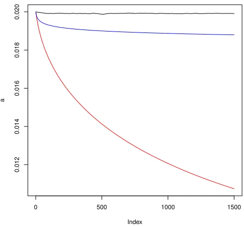
To illustrate our derived convergence rates and compare with the existing literature, we carry out numerical simulations corresponding to Example 2 with the same data distribu-tions as in (Needell, 2010): m= 200, d= 100, A∈R200×100 is a Gaussian matrix with each entry drawn independently from the standard normal distributionN(0,1), andy∈R100 is a Gaussian noise with each component drawn independently from the normal distribution with mean 0 and standard deviation 0.02. The measurement vectors {ψt = kϕ1tkϕt} are drawn from the normalized rows of A as in Example 2 and {yet = yt/kϕtk} with mean
x∗ = 0. We conduct 100 trials for each choice of the relaxation parameter sequences
ηt = 1, ηt = 1/
√
t, ηt = 1/t. In each trial, algorithm (4) is run 100 times with random
Gaussian initial vectors of norm kx1k = 0.02. Figure 1 depicts the error kxt+1−x∗k for
t= 1, . . . ,1500 (averaged with 100 trials and 100 initial vectors). The black line is a plot with the constant relaxation parameter sequenceηt= 1, which verifies the divergence of the
algorithm, as proved in (Needell, 2010). The blue line is a plot withηt= 1/
√
t, which hints a slow convergence of the algorithm. The red line is a plot withηt= 1/t, which confirms a
faster convergence. The above simulations are consistent with our error analysis.
In this paper, a learning theory approach to the relaxed randomized Kaczmarz algorithm is presented. It yields new results and observations including a necessary and sufficient condition (9), stated in Theorem 3, for the convergence in expectation when the sampling process is noisy or nonlinear. For noise-free and linear sampling processes (that is,E(fH) =
0), we can see from Remark 11 withηt≡1 thatEz1,...,zT[kxT+1−x
∗k2]≤ kx
1−x∗k2(1−λr)T.
0 500 1000 1500
0.012
0.014
0.016
0.018
0.020
Index
a
Figure 1: Error of the relaxed randomized Kaczmarz algorithm with ηt = 1 (black line),
ηt= 1/
√
1−λr is replaced by a quantity involving kA−1k= inf{M :MkAxk ≥ kxk for all x}. Our
result is more general (valid for underdetermined systems with kA−1k=∞).
In the framework of Kaczmarz algorithms, we consider online learning algorithms asso-ciated with the least squares loss. It would be interesting to extend our study to algorithms associated with more general loss functions (Ying and Zhou, 2006) such as hinge loss, and to consider error analysis without requiring the approximation error (Ying and Zhou, 2006) tending to zero.
Acknowledgments
The work described in this paper is supported partially by the Research Grants Council of Hong Kong [Project No. CityU 104113]. The authors would like to thank the referees for constructive suggestions and Dr. Xin Guo for helping with the numerical simulations. The corresponding author is Ding-Xuan Zhou.
References
X. Chen and A. Powell. Almost sure convergence for the Kaczmarz algorithm with random measurements. Journal of Fourier Analysis and Applications, 18:1195–1214, 2012.
T. Hu, J. Fan, Q. Wu, and D. X. Zhou. Regularization schemes for minimum error entropy principle. Analysis and Applications, 13:437–455, 2015.
J. Johnston.Econometric Methods. McGraw Hill, New York, 1963.
S. Kaczmarz. Angen¨aherte aufl¨osung von systemen linearer gleichungen. Bulletin
Interna-tional de l‘Acad´emie Polonaise des Sciences et des Lettres A, 35:355–357, 1937.
A. Klenke.Probability Theory: A Comprehensive Course. Springer-Verlag, London, 2008.
D. Needell. Randomized Kaczmarz solver for noisy linear systems. BIT. Numerical
Mathe-matics, 50:395–403, 2010.
I. Pinelis. Optimum bounds for the distributions of martingales in banach spaces. Annals
of Probability, 22:1679–1706, 1994.
Y. Ying and M. Pontil. Online gradient descent learning algorithms.Foundations of
Com-putational Mathematics, 8:561–596, 2008.
S. Smale and Y. Yao. Online learning algorithms. Foundations of Computational
Mathe-matics, 6:145–170, 2005.
S. Smale and D. X. Zhou. Online learning with Markov sampling.Analysis and Applications, 7:87–113, 2009.
P. Tarr´es and Y. Yao. Online learning as stochastic approximations of regularization paths.
IEEE Transactions on Information Theory, 60:5716–5735, 2014.
V. Vapnik. Statistical Learning Theory. John Wiley & Sons, 1998.
Y. Ying and D. X. Zhou. Online regularized classification algorithms. IEEE Transactions
on Information Theory, 52:4775–4788, 2006.
A. Zouzias and N. M. Freris. Randomized extended Kaczmarz for solving least squares.