Cross-Validation Optimization for Large Scale Structured
Classification Kernel Methods
Matthias W. Seeger [email protected]
Max Planck Institute for Biological Cybernetics Spemannstr. 38
T¨ubingen, Germany
Editor: Zoubin Ghahramani
Abstract
We propose a highly efficient framework for penalized likelihood kernel methods applied to multi-class models with a large, structured set of multi-classes. As opposed to many previous approaches which try to decompose the fitting problem into many smaller ones, we focus on a Newton opti-mization of the complete model, making use of model structure and linear conjugate gradients in order to approximate Newton search directions. Crucially, our learning method is based entirely on matrix-vector multiplication primitives with the kernel matrices and their derivatives, allow-ing straightforward specialization to new kernels, and focusallow-ing code optimization efforts to these primitives only.
Kernel parameters are learned automatically, by maximizing the cross-validation log likelihood in a gradient-based way, and predictive probabilities are estimated. We demonstrate our approach on large scale text classification tasks with hierarchical structure on thousands of classes, achieving state-of-the-art results in an order of magnitude less time than previous work.
Parts of this work appeared in the conference paper Seeger (2007).
Keywords: multi-way classification, kernel logistic regression, hierarchical classification, cross validation optimization, Newton-Raphson optimization
1. Introduction
In recent years, machine learning researchers started to address problems with kernel machines which require models with a large number of dependent variables, and whose fitting demand train-ing samples with very many cases. For example, for multi-way classification models with a hierar-chically structured label space (Cai and Hofmann, 2004), modern applications call for predictions on thousands of classes, and very large data sets become available. However, if n and C denote data set size and number of classes respectively, nonparametric kernel methods like support vector machines (SVMs) or Gaussian processes (GPs) typically scale super-linearly in nC, if dependencies between the latent class functions are represented properly.
We propose a general framework for learning in probabilistic kernel classification models. While the models treated here are not novel, a major feature of our approach is the high compu-tational efficiency with which the primary fitting (for fixed hyperparameters) is done. For example, our framework applied to hierarchical classification with hundreds of classes and thousands of data points requires a few minutes for fitting. The central idea is to step back from what seems to be the dominating approach in machine learning at the moment, namely to solve a large convex opti-mization problem by iteratively solving very many small ones. A popular approach for these small steps is to minimize the criterion w.r.t. a few variables only, keeping the other ones fixed, and many variations of this theme have been proposed. In this paper, we focus on the opposite approach of trying to find directions which lead to fast descent, no matter how many of the variables are in-volved. This is essentially Newton’s method, and one aspect of our work is to find approximate Newton directions very efficiently, making use of model structure and linear conjugate gradients in order to reduce the computation to standard linear algebra primitives on large contiguous chunks of memory. Interestingly, such global approaches are generally favoured in the optimization com-munity for problems (such as kernel methods fitting) which cannot be decomposed naturally into parts. While other gradient-based optimizers such as scaled conjugate gradients could be used as well, they require more fine-tuning (for example, preconditioning) to the specific problem they are applied to, while Newton’s method is closer to a “black box” technique and can be transferred to novel situations without many changes.
For multi-way classification, our primary fitting method scales linearly in C, and depends on n mainly via a fixed number of matrix-vector multiplications (MVM) with n×n kernel matrices. In many situations, these MVM primitives can be computed very efficiently, often without having to store the kernel matrices themselves.
We also show how to choose hyperparameters automatically by maximizing the cross-validation log likelihood, making use of our primary fitting technology as inner loop in order to compute the CV criterion and its gradient. It is important to note that our hyperparameter learning method works by gradient-based optimization, where the dominating part of the gradient computation does not scale with the number of hyperparameters at all.1 The gradient computation also requires a number of MVMs with derivatives of kernel matrices, which can be reduced to kernel MVMs for many frequently used kernels (see Section 7.3). Therefore, our approach can in principle be used to learn a large number of hyperparameters without user interaction.
We apply our framework to hierarchical classification with many classes. The hierarchy is represented through an ANOVA setup. While the C latent class functions are fully dependent a priori, the scaling of our method stays close to what unstructured (flat) classification with C classes would require. We test our framework on the same tasks treated by Cai and Hofmann (2004), achieving comparable results in at least an order of magnitude less time.
Our proposal to use approximate Newton methods is not novel as such. The Newton method, or a variant of it called Fisher scoring, is the standard approach for fitting generalized linear models in statistics (Green and Silverman, 1994; McCullach and Nelder, 1983), at least if parametric models are fitted to moderately sized samples. Our primary fitting method for flat multi-way classification (see Section 2) appeared in Williams and Barber (1998). However, we demonstrate the usefulness of this principle on a much larger scale, showing how model structure can (and has to) be exploited
in this context. Furthermore, we demonstrate how the secondary task of hyperparameter learning can be reduced to the same underlying primitives.
The structure of the paper is as follows. Our model and method of parameter fitting is given in Section 2. An extension to hierarchical classification is provided in Section 3, and in Section 4 we give our automatic hyperparameter learning procedure. Essential computational details are dis-cussed in Section 5. Experimental results on a very large hierarchical text classification and several standard machine learning problems are given in Section 6. We close with a discussion in Section 7, relating our global direction approach to popular block coordinate descent techniques in Section 7.2, and pointing out future work in Section 7.4.
Optimized C++ software for our framework is available as part of theLHOTSEtoolbox for adap-tive statistical models, which is freely available for non-commercial purposes.2The implementation contains the linear kernel case used in Section 6.1 (see Appendix D.3), as well as a generic represen-tation described in Appendix D.1, with which the experiments in Section 6.2, Section 6.3 have been done. It is fairly simple to include new kernels or (approximate) kernel MVM implementations.
2. Penalized Multiple Logistic Regression
In this section, we introduce our framework on a multi-way classification model with C classes, where structure between classes is not modelled. We refer to this setup as flat classification, in that the label set is flat (unstructured).
log P(y | u)
log P(u)
likelihood
coupling
u
1u
2. . .
u
Clatent
dependent
functions
"prior" mixing (optional)
latent
independent
functions
+
penalization
. . .
u
1u
2u
P( ( (
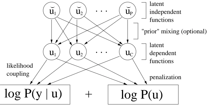
Figure 1: Structure of penalized likelihood optimization.
In general, our framework is applicable to models of the form depicted in Figure 1. A set of latent (unobserved) functions uc(·)is fitted to observed data by penalized likelihood maximization. For many models, the penalisation term (also called regulariser) corresponds to the logarithm of a prior density over the uc(·). This primary fitting step corresponds to a convex optimization problem over finitely many variables. Structure in such models is represented either as couplings in the log
likelihood function, or in the penalisation (or log prior) term. The latter can be realized through the linear mixing of a priori independent functions ˘up(·), in other words the penaliser over the latter decouples w.r.t. p (our main example of such mixing is hierarchical classification, developed in Section 3).
We now apply this general framework to flat classification, where y∈ {1, . . . ,C} is to be pre-dicted from x∈
X
, given some i.i.d. data D={(xi,yi)|i=1, . . . ,n}. Our notation convention for vectors and matrices is detailed in Appendix A, where we also collect all major notational definitions in a table. We code yi as yi∈ {0,1}C, 1Tyi=1 (zero-one coding).3 We employ the multiple logistic regression model, consisting of C latent class functions uc(·)feeding into the multiple logistic (or softmax) likelihood P(yic=1|xi,ui(·)) =euc(xi)/(∑c0euc0(xi)).We write uc(·) = fc(·) +bc for intercept (or bias) parameters bc∈Rand functions fc(·)living in a reproducing kernel Hilbert space (RKHS) with kernel K(c)=K(c)(·,·)(Sch¨olkopf and Smola, 2002), and consider the penalized negative log likelihood
Φ=−
n
∑
i=1
log P(yi|ui) + (1/2) C
∑
c=1
kfc(·)k2c+ (1/2)σ−2kbk2, ui= (uc(xi))c∈RC,
which we minimize for primary fitting. Here,k · kc is the RKHS norm for kernel K(c). The idea is that deviations in fc from desired functional properties encoded in K(c)are penalized by a large
kfc(·)k2c. For example, for the Gaussian kernel (7), non-smooth fcare penalized, and for the linear kernel (Appendix D.3), kfc(·)k2c is the squared norm of the weight vector. Details on penalized likelihood kernel methods and RKHS penalisation can be found in Green and Silverman (1994) and Sch¨olkopf and Smola (2002).
The model can also be understood in a Bayesian context, where the penalisation terms come from zero mean Gaussian process priors on the functions fc(·), and b has a zero mean Gaussian prior with varianceσ2. From this viewpoint, we do a maximum a-posteriori (MAP) approximation here, without however taking covariances into account properly (which would be much more expensive to do). Details on Gaussian processes for machine learning can be found in Seeger (2004) and Rasmussen and Williams (2006).
Since the likelihood depends on the fc(·) only through the values fc(xi) at the data points, every minimizer ofΦmust be a kernel expansion: fc(·) =∑iαicK(c)(·,xi). This fact is known as representer theorem (Green and Silverman, 1994; Wahba, 1990). Plugging this in, the regulariser becomes(1/2)αTKα+ (1/2)σ−2kbk2, where K(c)= (K(c)(x
i,xj))i,j∈Rn,n, and K=diag(K(c))cis block-diagonal. The kernels K(c)can in general be different, although sharing kernels among classes can lead to computational savings, in that some of the blocks K(c)are identical. Our implementation of block sharing is described in Appendix D.1.
We show in Section 5.1.1 that the bc may be eliminated as b =σ2(I⊗1T)α. Thus, if ˜K = K+σ2(I⊗1)(I⊗1T), then our criterionΦbecomes
Φ=Φlh+ 1 2α
TKα˜ , Φ
lh=−yTu+1Tl, li=log 1Texp(ui), u=K˜α. (1)
Φ is strictly convex in α, being a sum of linear, quadratic, and logsumexp terms of the form log 1Texp(ui)(Boyd and Vandenberghe, 2002), so it has a unique minimum point ˆα. The
sponding kernel expansions are
ˆ
uc(·) =
∑
i ˆ
αic(K(c)(·,xi) +σ2).
Estimates of the conditional probability on test points x∗ are obtained by plugging ˆuc(x∗) into the likelihood. These estimates are asymptotically consistent, although better finite sample estimates could probably be obtained by a more Bayesian treatment.
We note that this setup is related to the multi-class SVM (Crammer and Singer, 2001), where
−log P(yi|ui)is replaced by the margin loss−uyi(xi) +maxc{uc(xi) +1−δc,yi}. Here,δa,b=I{a=b}. The negative log multiple logistic likelihood has similar properties, but is smooth as a function of
u, and the primary fitting of α does not require constrained convex optimization. Furthermore,
universal consistency for estimates of P(y∗|x∗)can be established for the multiple logistic loss, but fails to hold for the SVM variant (Bartlett and Tewari, 2004).
We will minimizeΦ using the Newton-Raphson (NR) algorithm. The computation of Newton search directions requires solving a system with the Hessian and the gradient ofΦ, which we will do approximately using the linear conjugate gradients (LCG) algorithm. This can be done without fully computing, storing, or inverting the Hessian, all of which would not be possible for large nC. In fact, the task is reduced to computing k1(k2+2)MVMs with K , where k1is the number of NR iterations, k2the number of LCG steps for computing each Newton direction. Since NR is a second-order convergent method, k1is generally small. k2determines the quality of each Newton direction, and again, fairly small values seem sufficient (see Section 6.1). Details are provided in Section 5.1. Finally, some readers may wonder why we favour the NR algorithm here, which in practice can be fairly complicated to implement, while we could do a simpler gradient-based optimization ofΦ w.r.t.α, for example by scaled (non-linear) conjugate gradients (SCG). The problem is that on tasks of the size we want to address, non-invariant methods such as SCG tend to fail completely if not properly preconditioned, and we experienced exactly that in preliminary experiments. In contrast to that, NR is invariant to the choice of optimization variables, so does not have to be preconditioned. It is by far the preferred method in the optimization literature (Bertsekas, 1999; Boyd and Vanden-berghe, 2002), and many ideas for preconditioning or Quasi-Newton try to approximate the NR directions. We think that a proper SCG implementation can be at least as efficient as NR, but needs fine-tuning to the specific problem, which in the case of hierarchical classification (discussed next) is already quite difficult. More details on this point are given in Section 5.4 and also Section 7.2.
3. Hierarchical Classification
So far we dealt with flat classification, the classes being independent a priori, with block-diagonal kernel matrix K . However, if the label set has a known structure,4we can benefit from representing it in the model. Here we focus on hierarchical classification, the label set{1, . . . ,C}being the leaf nodes of a tree. Classes with lower common ancestor should be more closely related. In this section, we propose a model for this setup and show how it can be dealt with in our framework with minor modifications and reasonable extra cost.
In flat classification, the latent class functions uc(·) are modelled as a priori independent, in that the penaliser (or the log prior in the GP view) is a sum of individual terms for each c, without
1
4
5
6
7
8
3
0
2
6 6 3
u = u + u
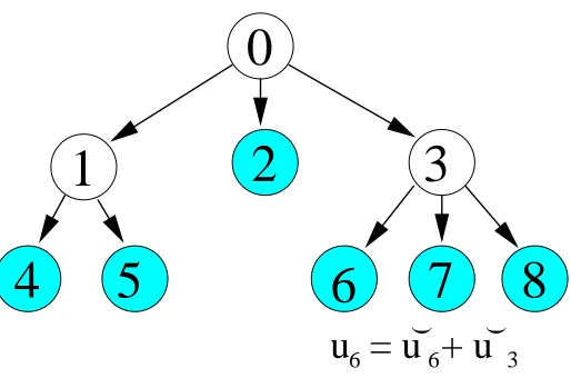
( (Figure 2: Example of a tree-structured target space, where labels correspond to leaf nodes (shaded).
interaction terms. Analysis of variance (ANOVA) models go beyond such independent designs, they have previously been applied to text classification by Cai and Hofmann (2004), see also Shahbaba and Neal (2007). Let {0, . . . ,P} be the nodes of the tree, 0 being the root, and the numbers are assigned breadth first (1,2, . . . are the root’s children). The tree is determined by P and np, p= 0, . . . ,P, the number of children of node p. Let L be the set of leaf nodes,|L|=C. Assign a pair of latent functions up,u˘p to each node, except the root. The ˘upare assumed a priori independent, as in flat classification. up is the sum of ˘up0, where p0 is running over the nodes (including p) on
the path from the root to p. An example is given in Figure 2. The class functions to be fed into the classification likelihood are the uL(c) of the leafs. This setup represents similarities according
to the hierarchy. For example, if leafs L(c),L(c0) have the common parent p, then uL(c)=up+ ˘
uL(c), uL(c0)=up+u˘L(c0), so the class functions share the effect up. Since regularisation forces all
independent effects ˘up0 to be smooth, the classes c,c0are urged to behave similarly a priori.
Let u= (up(xi))i,p, ˘u= (u˘p(xi))i,p∈RnP. The vectors are linearly related as u= (Φ⊗I)˘u,Φ∈
{0,1}P,P, a special case of the mixing of Figure 1. Importantly, Φ has a simple structure which allows MVM withΦ orΦT to be computed easily in O(P), without having to compute or storeΦ explicitly. Let csp=∑p0<pnp0, and defineΦp∈Rd,d,d =csp+np, to be the upper left block of
Φ, so thatΦ=ΦP. If p is a leaf node, thenΦp=Φp−1. Otherwise,Φpis obtained fromΦp−1 by attaching rows(δTpΦp−1,δTj),j=1, . . . ,np, whereδTpΦp−1is the p-th row ofΦp−1. This is because ucsp+j=up+u˘csp+jfor the functions of the children of p. Formally,
Φp=
Φ
p−1 0 1δT
pΦp−1 I
,
where the lower right I ∈Rnp,np. Note thatΦ is lower triangular with diagΦ =I. This recursive definition directly implies simple methods for computing v7→Φv and v7→ΦTv.
Under the hierarchical model, the class functions uL(c) are strongly dependent a priori. Rep-resenting this prior coupling in our framework amounts to simply plugging in the implied kernel matrix
into the flat classification model of Section 2. Here, the inner ˘K is block-diagonal, while in the flat model, K itself had this property. In the hierarchical case, K is not sparse and certainly not block-diagonal, but we are still able to compute kernel MVMs efficiently: pre- and post-multiplying byΦ is very cheap, and ˘K is block-diagonal just as in the flat case.
In fact, the step from flat to hierarchical classification requires minor modifications of existing code only. If code for representing a block-diagonal K is available, we can use it to represent the inner ˘K , just replacing C by P. This simplicity carries through to the hyperparameter learning method (see Section 4). The cost of a kernel MVM is increased5by a factor P/C<2, which in most hierarchies in practice is close to 1.
However, it would be wrong to claim that hierarchical classification in general comes as cheap as flat classification. In fact, primary fitting becomes more costly, precisely because there is more coupling between the variables. In the flat case, the Hessian ofΦ (1) is close to block-diagonal. The LCG algorithm to compute Newton directions converges quickly, because it nearly decom-poses into C independent ones, and fewer NR steps are required. In the hierarchical case, this “near-decomposition” does not hold, and both LCG and NR need more iterations to attain the same accuracy, although each LCG step comes at about the same cost as in the flat case.
In numerical mathematics, much work has been done to approximately decouple linear systems by preconditioning. In some of these strategies, knowledge about the structure of the system matrix (in our case: the hierarchy) can be used to drive preconditioning. An important point for future re-search is to find a good preconditioning strategy for the system (5). However, in all our experiments so far the fitting of the hierarchical model took less than twice the time required for the flat model on the same task.
4. Hyperparameter Learning
Our framework comes with an automatic method for setting free hyperparameters h, by gradient-based maximization of the cross-validation (CV) log likelihood. Our primary fitting method of Section 2 is used here as principal subroutine. Such a setup is commonplace in Bayesian statistics, where (marginal) inference is typically employed as subroutine in parameter learning.
Recall that primary fitting works by minimizingΦ(1) w.r.t.α. Let{Ik}be a partition of the data set range{1, . . . ,n}, with Jk={1, . . . ,n} \Ik, and let
ΦJk =u T
[Jk]((1/2)α[Jk]−yJk) +1
Tl
[Jk]
be the negative log likelihood of the subset Jk of the data. Here, u[Jk] =K˜Jkα[Jk]. The α[Jk] are independent variables, not part of a common6α. The cross-validation criterion is
Ψ=
∑
k
ΨIk, ΨIk =−y T
Iku[Ik]+1 Tl
[Ik], u[Ik]=K˜Ik,Jkα[Jk], (3)
whereα[Jk] is the minimizer ofΦJk. Since for each k, we fit and evaluate the likelihood on disjoint parts of y,Ψis an unbiased estimator of the true negative expected log likelihood.
In order to adjust h, we pick a fixed partition at random, then do gradient-based minimization of Ψw.r.t. h. To this end, we maintain the set{α[Jk]}of primary variables, and iterate between re-fitting
5. Nodes with a single child only can be pruned from the hierarchy. Note that our formalism does not require all leaf nodes to have the same depth.
those for each fold k, and computingΨand∇hΨ. The gradient can be determined analytically, using a computation which is equivalent to the Newton direction computations forα[Jk], meaning that the same code can be used. Details are given in Section 5.2. Note thatΨis not a convex objective.
As for computational complexity, suppose there are q folds. The update of the α[Jk] requires q primary fitting applications, but since they are initialized with the previous valuesα[Jk], they do converge very rapidly, especially during later iterations. Computing Ψbased on the α[Jk] comes basically for free. The gradient computation decomposes into two parts: accumulation, and kernel derivative MVMs. The accumulation part requires solving q systems of size((q−1)/q)nC, thus q k3 kernel MVMs on the ˜KJk if linear conjugate gradients (LCG) is used, k3being the number of LCG steps. We also need two buffer matrices E,F of q nC elements each. Note that the accumu-lation step is independent of the number of hyperparameters. The second part consists of q kernel derivative MVMs for each independent component of h. This second part is much simpler than the accumulation one, consisting entirely of large matrix operations, which can be run very efficiently using specialized numerical linear algebra code. The method for computing Ψand ∇hΨcan be plugged into a custom gradient-based optimizer, such as Quasi-Newton or conjugate gradients, in order to learn h.
As shown in Section 5.3, the extension of hyperparameter learning to the hierarchical case of Section 3 is done by wrapping the accumulation part with Φ MVMs, the coding and additional memory effort being minimal.
We finally note from our findings in practice (see Section 6.3) that on large tasks, our automatic method can require some fine-tuning. This is due to the delicate dependencies between the different approximations used. The accuracy of Ψ and∇hΨ depends on how accurate the inner NR opti-mizations forα[Jk]turn out, and the latter depend on how many iterations of LCG are done in order to compute search directions. Fortunately,ΦJk and its gradient w.r.t. u[Jk]can be computed exactly in order to assess inner optimization convergence, so we do at least know when things go wrong. In our implementation, we deem an evaluation ofΨand∇hΨusable if the average ofk∇u[Jk]ΦJkk over folds is below a threshold, which depends on the problem and on time constraints. A failed evaluation leads to a right bracket there for the outer optimization line search, in that step sizes beyond the failed one are not accessed. We can now tune the basic running time parameters k1,k2 so thatΨevaluations do not fail too often. In this context, it is important to regard the {α[Jk]}as an inner state alongside the hyperparameter vector h. Although inner optimizations are convex, for large problems and reasonable k1,k2, successive minima are attained only when we start from the previous best inner state. This is true especially during later stages, where for certain problems (see Section 6.3) h attends “extreme” values and the inner optimizations become quite hard.7Therefore, the inner state used to initialize a givenΨevaluation is the final one for the last recent successful evaluation.8 Inner states attained during failed evaluations are discarded.
7. Although inner optimizations are convex, speed of convergence of NR depends strongly on the value of h. For “extreme” values, the Newton direction computation by LCG is harder, and search directions can become large in early NR iterations. The latter may be because we work in u rather thanαspace, but only the former is really feasible. 8. Within outer line searches, we use{α[Jk]}from the last recent successful evaluation to the left (along the search
5. Computational Details
In this section, we provide details for the material above. The techniques given here do characterize our framework, they are novel in this combination, and some of them may be useful in other contexts as well. More specific details of our implementation can be found in Appendix D.
5.1 Details for Flat Classification
In this section, we provide details for the primary fitting optimization in the case of flat multi-way classification, introduced in Section 2. Note that this fitting method appeared in Williams and Barber (1998) in the context of approximate Gaussian process inference, although some fairly essential ideas here are novel to our knowledge (symmetrisation of Newton system, pair optimization line search, numerical stability considerations).
Recall that we want to minimize the strictly convex criterionΦ(1) w.r.t.α, using the Newton-Raphson (NR) method. Modern variants of this algorithm iterate line searches along the Newton directions−H−1g, where g,H are gradient and Hessian ofΦ at the currentα. We will start with the Newton direction computation in Section 5.1.1, commenting on the line searches afterwards in Section 5.1.2 (it turns out that it basically comes for free). An overview of the fitting algorithm is given in Section 5.1.3.
5.1.1 COMPUTING THENEWTONDIRECTION
RecallΦand related variables from (1). Letπic=P(yic=1|ui),π=exp(u−1⊗l), and recall that Φlhis the likelihood part inΦ. Now,
g :=∇Φlh=π−y,W :=∇∇Φlh=D−DPclsD,Pcls= (1⊗I)(1T⊗I).
Here, D=diagπ, and gradient and Hessian are taken w.r.t. u (not w.r.t.α). Our convention for nC vectors and matrices and the use of⊗is explained in Appendix A. The form of W can be understood by noting that W is block-diagonal in a different ordering, which uses c (classes) as inner and i (data points) as outer index, then switching to our standard ordering.
It is easy to compute gradient and Hessian of Φ w.r.t.α,b. A full (classical) Newton step is given by the system
(I+W K)α0+W(I⊗1)b0=W u−g,
(I⊗1T)W Kα0+ (I⊗1T)W(I⊗1)b0+σ−2b0= (I⊗1T)(W u−g),
and the Newton search direction is obtained as the differenceα0−α,b0−b. Subtracting(I⊗1T)
times the first from the second, we obtain b0=σ2(I⊗1T)α0, and plugging this into the first equation, we have
I+W K+σ2Pdata
α0
=W u−g, Pdata= (I⊗1)(I⊗1T). (4)
Note that Pdataa= (∑i0ai0)i, which does the same as Pcls, but on index i rather than c. We denote
˜
K=K+σ2P data,
of “eliminating b” in Section 2. While we could optimizeσ2as a hyperparameter, we consider it fixed and given for simplicity.9 In the sequel, we consider b being eliminated from the model by replacing K→K everywhere. We have u˜ =K˜α.
We can solve the system (4) exactly if we can tolerate a scaling of O(n3C)and O(n2C)memory. Note that this scaling is linear rather than cubic in C. The exact solution is derived in Appendix C. It is efficient for moderate n, and generally useful for code debugging, and is supported by our implementation. In the remainder of this section, we focus on approximate computations.
Although we could solve the system using a bi-conjugate gradients solver, we can do much bet-ter by transforming it into symmetric positive definite form. First, note that W is positive semidef-inite, but singular. This can be seen by noting that the parameterization of our likelihood in terms of ui is overcomplete, in that ui+κ1 gives the same likelihood values for allκ. We could fix one of the ui components, which would however lead to subtle dependencies between the remaining C−1 functions uc(·). In order to justify our a priori independent treatment of these functions, we have to retain the overcomplete likelihood. The nullspace kerW is given by {(d)c|d ∈Rn} and has dimension n. This can be seen by noting that W a=0 iff a= (¯a)c, ¯a=∑c0a(c
0)
. W has rank n(C−1). We have a∈ranW iff ∑ca(c)= (1T⊗I)a =0 (recall that kerW and ranW are orthogonal, and their direct sum is RnC). From (4) we see that α0+g lies in ranW . Note that ∑cg(c)=∑c(π(c)−y(c)) =1−1=0, therefore g∈ranW , thusα0∈ranW . We see that the dual coefficients must fulfill the constraintα∈ranW . Note that ranW is in fact independent of D. What-ever starting value is used for α, it should be projected onto ranW , which is done by subtracting C−1Pclsα. The NR updates then make sure that the constraint remains fulfilled.
Next, we need a decomposition W =V VTof W . Such a V exists (because W is positive semidef-inite). In fact,
W =ADAT, A=I−DPcls.
This follows easily from(1T⊗I)D(1⊗I) =∑c0D(c 0)
=I. Thus, W =V VT with V =AD1/2. The
matrix A has fixed points ranW , namely if a∈ranW , then(1T⊗I)a=0, so that Aa=a. Since there exists some ˜v (not unique) s.t.α0=W ˜v, we can rewrite the system (4) as
V I+VTKV˜ VT˜v=V VTu−˜g,
where ˜g is s.t. g=V ˜g (such a vector exists because g∈ranW ). This suggests the following proce-dure for findingα0:
I+VTKV˜ β
=VTu−˜g, α0=Vβ. (5)
To see the validity of this approach, simply multiply both sides of (5) by V from the left, which shows that Vβsolves the original system. Since the latter has a unique solution (strict convexity!), we must have Vβ=α0. Finally, we note that ˜g=D−1/2g does the job, because V D−1/2g=Ag=g. The latter follows because g∈ranW .
Thus, in exact arithmetic, the Newton direction computation is implemented in a three-stage procedure. First, compute ˜g=D−1/2g. Second, solve the system (5) for β. This is a symmetric positive definite system with the typically well-conditioned matrix I+VTKV , and can be solved˜ efficiently using the linear conjugate gradients (LCG) algorithm (Saad, 1996). The cost of each step is dominated by the MVM v7→K v, which scales linearly in C, due to the block-diagonal structure of K . Third, setα0=Vβ. The Newton direction is obtained asα0−α.
We can start the LCG run from a good guess as follows. Letαbe the current dual vector which solved the last recent system. We would like to initializeβ s.t.α=Vβ=AD1/2β. If we assume that D1/2β∈ranW , thenα=D1/2β. Therefore, a good initialization isβ=D−1/2α. Alternatively, we may also retainβfrom the last recent system.
Issues of numerical stability are addressed in Appendix B. Furthermore, the LCG algorithm is hardly ever run without some sort of preconditioning. Our present implementation uses diagonal preconditioning, as described in Appendix B. We have already noted in Section 3 that a non-diagonal preconditioning strategy could be valuable, but this is subject to future work.
5.1.2 THELINESEARCH
The classical NR algorithm proceeds doing full stepsα→α0, but modern variants typically employ a line search along the Newton directionα0−α. In the non-convex case, this ensures global
con-vergence, and even for our convex objective Φ, a line search saves time and leads to numerically more stable behaviour. Interestingly, the special structure of our problem leads to the fact that line searches essentially come for free, certainly compared with the effort of obtaining Newton direc-tions. We refer to this simple idea as pair optimization, the reader may be reminded of similar tricks in primal-dual schemes for SVM.
Let s=α0−αbe the NR direction, computed as shown above, and setα0toα. The line search minimizes (or sufficiently decreases)Φon the line segmentα0+λs,λ∈(0,1], starting withλ=1 (which is the classical Newton step). The idea is to treatΦas a function of the pair(u,α), where u=Kα. The corresponding line segment is u˜ =u0+λ˜s, ˜s=K s, requiring a single kernel MVM˜ for computing ˜s. Let j=argmax|s˜j|. For an evaluation ofΦat u, we reconstructλ= (uj−u0,j)/s˜j andα=α0+λs, then
Φ=uT((1/2)α−y) +1Tl, ∇Φ=π−y+α,
so that an evaluation comes at the cost O(nC) and does not require additional kernel MVM ap-plications. We now do the line minimization of Φ in the variable u. The driving feature of pair optimization is that we can go back and forth betweenα and u without significant cost, once the search direction is known w.r.t. both variables.
5.1.3 OVERVIEW OF THE OPTIMIZATIONALGORITHM
In Algorithm 1, we give a schematic overview of the primary fitting algorithm, written in terms of a MVM primitive v7→K v. For simplicity, we do not include the measures discussed in Appendix B to increase numerical stability.
5.2 Details for Hyperparameter Learning
In this section, we provide details for the CV hyperparameter learning scheme, introduced in Sec-tion 4. The gradient of the CV criterionΨ(3) is computed as follows.Ψis a sum of termsΨIk, one for each fold. We focus on a single term and write I=Ik,J=Jk.α[J]is determined by the stationary
equationα[J]+g[J]=0 (all terms of subscript[J]are as in Section 5.1.1, but for the subset J of the
data, and w.r.t.α[J]). Taking derivatives gives
dα[J]=−W[J] (dKJ)α[J]+K˜J(dα[J])
Algorithm 1 Newton-Raphson optimization to find posterior mode ˆα. Require: Starting values forα,b. Targets y.
α=α−C−1(∑c0α(c 0)
)c, so thatα∈ranW . u=Kα.˜
repeat
Compute l,log(π)from u. ComputeΦ.
if relative improvement inΦsmall enough then Terminate outer loop.
else if maximum number of iterations done then
Terminate outer loop.
end if
Initializeβ=D−1/2α. Compute r.h.s. r=VTu−˜g, ˜g=D−1/2g. Compute preconditioner diag(I+VTKV˜ ).
Run preconditioned CG algorithm in order to solve the system (5) approximately. The CG code is configured by a primitive to compute v7→(I+VTKV˜ )v, which in turn calls the primitive for v7→K v.
Computeα0=AD1/2β0.
Do line search along s=α0−α. This is done in u, along ˜s=K s.˜ Assign line minimizer toα,u.
until forever
since dg[J]=W[J]du[J]. We obtain a system for dα[J]which is symmetrised as in Section 5.1.1:
I+VT[J]K˜JV[J]
β=−VT[J](dKJ)α[J], dα[J]=V[J]β.
Also,
dΨI= π[I]−yI
T
((dKI,J)α[J]+K˜I,J(dα[J])).
With
f =I·,I(π[I]−yI)−I·,JV[J]
I+VT[J]K˜JV[J]
−1
VT[J]K˜J,I(π[I]−yI),
we have that dΨI= (I·,Jα[J])T(dK)f .
If we collect these vectors as columns of E,F ∈RnC,q, q the number of folds, we have that
dΨ=tr ET(dK)F (6)
many hyperparameters. For moderately many hyperparameters, the accumulation clearly dominates the CV criterion and gradient computation.
The dominating part of the accumulation is the re-optimisation of theα[J], which are done by
calling the optimized code for primary fitting (Section 5.1) as subroutine. Here, a feature of our implementation becomes important. Instead of representing each KJk separately, we represent the full K only for all subset kernel MVMs. The representation depends on the covariance function, and in general on how kernel MVMs are actually done. A generic representation is described in Appendix D.1. In order to work on the data subset Jk, we shuffle the representation such that in the permuted kernel matrix, KJk forms the upper left corner. This means that linear algebra primitives with KJk can be run without mapping matrix coordinates through an index, which would be many times slower. Details on “covariance shuffling” are given in Appendix D.2.
As mentioned in Section 5.1.1 and detailed in Appendix C, we can also compute Newton direc-tions exactly in O(C n3)in the flat classification case. This exact treatment can be extended to the computation ofΨ and its gradient, as is shown in Appendix C. Exact computations lead to more robust behaviour, and may actually run faster for small to moderate n. Exact computations are also useful for debugging purposes.
5.3 Details for Hierarchical Classification
In this section, we provide details for hierarchical classification method, introduced in Section 3. Recall that u= (Φ⊗I)˘u for an indicator matrixΦof simple structure, and that MVM withΦorΦT can be computed easily in O(P), without having to storeΦ. Since the ˘up(·)are given independent priors (or regularisers), the corresponding kernel matrix ˘K is block-diagonal. The induced covari-ance matrix K over uL is given by (2), and hierarchical classification differs from the flat variant only in that this non-block-diagonal matrix is used.
The MVM primitive v 7→K v is computed in three steps. MVM with(ΦL,·⊗I)and(ΦTL,·⊗I) works by computing S7→SΦ,S7→SΦT for S∈Rn,P. In between, MVM with ˘K has to be done in the same way as for flat classification, only that ˘K has P rather than C diagonal blocks.
The diagonal preconditioning of LCG (see Appendix B) requires the computation of diag K ∈
RnC. We have
Kic,ic= (δTpΦ⊗δTi )K˘(ΦTδp⊗δi) =δTpΦ(diag(K˘
(p0)
i )p0)ΦTδp, p=L(c),
whereδTpΦ is the p-th row ofΦ. From the recursive structure ofΦ we know that if np>0, then δT
csp+jΦ=δ T pΦ+δ
T
csp+j, j=1, . . . ,np, so if
di(csp+j)=dip+K˘
(csp+j)
i , j=1, . . . ,np,
then diag K=dL.
Hyperparameter learning (see Section 5.2) is easily extended to the hierarchical case, recalling (2) and the fact thatΦ does not depend on hyperparameters. Define ˜E = (ΦT
withΦ andΦT respectively, calling the existing “flat” primitives for ˘K in between (block-diagonal with P rather than C blocks).
5.4 Why Newton Raphson?
Why do we propose to use the second-order NR method for minimizing Φ, instead of using a simpler gradient-based technique such as scaled conjugate gradients (SCG)? We already motivated our choice at the end of Section 2, but give more details concerning this important point here.
The convex problems we are interested in here live in very high-dimensional spaces and come with complicated couplings between the components which cannot be characterized simply. Cer-tainly, there is no simple decomposition into parts. It is well known in the optimization literature (Bertsekas, 1999) that simple gradient-based techniques such as SCG require well-chosen precon-ditioning in order to work effectively in such cases.
For example, we could optimizeΦ(1) w.r.t.αdirectly, the gradient requires a single MVM with K rather than solving a system. However, this problem is very ill-conditioned, the Hessian being
˜
KW ˜K+K (large kernel matrices are typically very ill-conditioned, and here we deal with K˜ 2), and SCG runs exceedingly slowly to the point of being essentially useless (as we determined in exper-iments). It can be saved (to our knowledge) only by preconditioning, which in our case requires to solve a system again. Another idea is to optimizeΦ w.r.t. u by SCG, which works better. The Hessian is W+K˜−1, whose condition number is similar to K . In preliminary direct comparisons, the NR method still works more efficiently, meaning that SCG would require additional precon-ditioning specific to the problem at hand, which would likely be different for flat and hierarchical classification. From our experience, and also from the predominance of NR in the optimization literature, we opted for this method which comes with self-tuning capabilities, making it easier to transfer the framework to novel problems.
6. Experiments
In this section, we provide experimental results for our method on a range of flat and hierarchical classification tasks.
6.1 Hierarchical Classification: Patent Texts
We use the WIPO-alpha collection,10 many thanks to L. Cai, T. Hofmann for providing us with the count data and dictionary. We did Porter stemming, stop word removal, and removal of empty categories. The attributes are bag-of-words over the dictionary. All input vectors xiwere scaled to unit norm. Many thanks to Peter Gehler for helping us with the preprocessing.
These tasks have previously been studied by Cai and Hofmann (2004), where patents (title and claim text) are to be classified w.r.t. the standard taxonomy IPC, a tree with 4 levels and 5229 nodes. Sections A, B,. . ., H form the first level. As in Cai and Hofmann (2004), we concentrate on the 8 subtasks rooted at the sections, ranging in size from D (n=1140,C=160,P=187) to B (n=9794,C=1172,P=1319). We use linear kernels (see Appendix D.3) with variance parameters vc.
All experiments are averaged over three training/test splits, different methods using the same ones. The CV criterion Ψis used with a different (randomly drawn) 5-partition per section and
split, the same across all methods. Our method outputs a predictive distribution pj ∈RC for each test case xj. The standard prediction y(xj) =argmaxcpjcmaximizes expected accuracy, classes are ranked as rj(c)≤rj(c0) iff pjc≥pjc0, where rj(c)∈ {1, . . . ,C} is the rank of class c for case xj.
Let yj denote the true label for xj. The test scores we use here are the same as in Cai and Hofmann (2004): accuracy (acc) m−1∑jI{y(xj)=yj}, precision (prec) m
−1∑
jrj(yj)−1, parent accuracy (pacc) m−1∑jI{par(y(xj))=par(yj)}, par(c)being the parent of leaf node L(c)(recall that L(c)corresponds to class c). Here, m is the test set size. Let ∆(c,c0) be half the length of the shortest path between leafs L(c),L(c0). The taxo-loss (taxo) is m−1∑j∆(y(xj),yj). These scores are motivated in Cai and Hofmann (2004). For taxo-loss and parent accuracy, we better choose y(xj)to minimize expected loss,11 which is different in general than the standard prediction (the latter maximizes expected accuracy and precision).
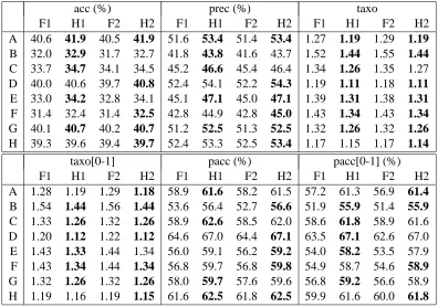
We compare methods F1, F2, H1, H2 (F: flat, not using IPC; H: hierarchical). F1: all vcshared (1); H1: vc shared across each level of the tree (3). F2, H2: vc shared across each subtree rooted at root’s children (A: 15, B: 34, C: 17, D: 7, E: 7, F: 17, G: 12, H: 5). The numbers in parentheses are the total number of hyperparameters. Recall that there are three parameters determining the running time (see Section 2, Section 4). For hyperparameter learning: k1=8,k2=4,k3=15 (F1, F2); k1=10,k2=4,k3=25 (H1, H2).12 For the final fitting (after hyperpars have been learned): k1=25,k2=12 (F1, F2); k1=30,k2=17 (H1, H2). The optimization is started from vc=5 for all methods. We setσ2=0.01 throughout. Results are given in Table 1.
The hierarchical model outperforms the flat one consistently, especially w.r.t. taxo-loss and par-ent accuracy. Also, minimizing expected loss is consistpar-ently better than using the standard rule for the latter, although the differences are not significant. H1 and H2 do not perform differently: choos-ing many different vcin the linear kernel seems no advantage here (but see Section 6.2). The results are quite similar to the ones of Cai and Hofmann (2004), obtained with a support vector machine variant. However, for our method, the recommendation in Cai and Hofmann (2004) to use vc=1 (not further motivated there) leads to significantly worse results in all scores. The vcchosen by our method are generally larger. Note that their code has not been made publicly available, so a direct comparison with “all other things equal” could not be done.
In Table 2, we present running times13 for the final fitting and for a single fold during hyper-parameter optimization (5 of these are required forΨ, ∇hΨ). In comparison, a final fitting time of 2200s on the D section is quoted in Cai and Hofmann (2004), using a SVM variant, while we require 119s (more than six times faster).14 It is precisely this high efficiency of primary fitting, which allows us to use it as inner loop for automatic hyperparameter learning (Cai and Hofmann, 2004, do not adjust hyperparameters to the data). Possible reasons for the performance difference are given in Section 7.2.
11. For parent accuracy, let p(j)be the node with maximal mass (under pj) of its children which are leafs, then y(xj)
must be a child of p(j).
12. Except for section C, where k1=14,k2=6,k3=35.
13. Processor time on 64bit 2.33GHz AMD machines.
acc (%) prec (%) taxo
F1 H1 F2 H2 F1 H1 F2 H2 F1 H1 F2 H2
A 40.6 41.9 40.5 41.9 51.6 53.4 51.4 53.4 1.27 1.19 1.29 1.19
B 32.0 32.9 31.7 32.7 41.8 43.8 41.6 43.7 1.52 1.44 1.55 1.44
C 33.7 34.7 34.1 34.5 45.2 46.6 45.4 46.4 1.34 1.26 1.35 1.27 D 40.0 40.6 39.7 40.8 52.4 54.1 52.2 54.3 1.19 1.11 1.18 1.11
E 33.0 34.2 32.8 34.1 45.1 47.1 45.0 47.1 1.39 1.31 1.38 1.31
F 31.4 32.4 31.4 32.5 42.8 44.9 42.8 45.0 1.43 1.34 1.43 1.34
G 40.1 40.7 40.2 40.7 51.2 52.5 51.3 52.5 1.32 1.26 1.32 1.26
H 39.3 39.6 39.4 39.7 52.4 53.3 52.5 53.4 1.17 1.15 1.17 1.14
taxo[0-1] pacc (%) pacc[0-1] (%)
F1 H1 F2 H2 F1 H1 F2 H2 F1 H1 F2 H2
A 1.28 1.19 1.29 1.18 58.9 61.6 58.2 61.5 57.2 61.3 56.9 61.4
B 1.54 1.44 1.56 1.44 53.6 56.4 52.7 56.6 51.9 55.9 51.4 55.9
C 1.33 1.26 1.32 1.26 58.9 62.6 58.5 62.0 58.6 61.8 58.9 61.6 D 1.20 1.12 1.22 1.12 64.6 67.0 64.4 67.1 63.5 67.1 62.6 67.0 E 1.43 1.33 1.44 1.34 56.0 59.1 56.2 59.2 54.0 58.2 53.5 57.9 F 1.43 1.34 1.44 1.34 56.8 59.7 56.8 59.8 54.9 58.7 54.6 58.9
G 1.32 1.26 1.32 1.26 58.0 59.7 57.6 59.6 56.8 59.2 56.6 58.9 H 1.19 1.16 1.19 1.15 61.6 62.5 61.8 62.5 59.9 61.6 60.0 61.8
Table 1: Results on patent text classification tasks A-H. Methods F1, F2 flat, H1, H2 hierarchical. taxo[0-1], pacc[0-1] for argmaxcpjcstandard prediction rule, rather than minimization of expected loss.
Final NR (s) CV Fold (s) Final NR (s) CV Fold (s)
F1 H1 F1 H1 F1 H1 F1 H1
A 2030 3873 573 598 E 131.5 203.4 32.2 49.6 B 3751 8657 873 1720 F 1202 2871 426 568 C 4237 7422 719 1326 G 1342 2947 232 579 D 56.3 118.5 9.32 20.2 H 971.7 1052 146 230
Table 2: Running times for tasks A-H. Method F1 flat, H1 hierarchical. Final NR: Final fitting with Newton-Raphson. CV Fold: Re-optimization ofα[J]and gradient accumulation for single
6.2 Flat Classification: Remote Sensing
We use the satimage remote sensing task from the statlog repository.15 This task has been used in the extensive SVM multi-class study of Hsu and Lin (2002), where it is among the data sets on which the different methods show the most variance. It has n=4435 training, m=2000 test cases, and C=6 classes. Covariates x have 36 attributes with values in {0, . . . ,255}. No preprocessing was done.
We use the isotropic Gaussian (RBF) covariance function
K(c)(x,x0) =vcexp
−wc
2 kx−x
0k2, v
c,wc>0. (7)
We compare the methods mc-sep (ours with separate kernels for each class; 12 hyperparameters), mc-tied (ours with a single shared kernel; 2 hyperparameters), mc-semi (ours with single kernel M(1), but different vc; 7 hyperparameters), 1rest (one-against-rest; 12 hyperparameters). For 1rest, C binary classifiers are fitted on the tasks of separating class c from all others. They are combined afterwards by the rule x∗7→argmaxcPˆc(+1|x∗), where ˆPc(+1|x∗)is the predictive probability esti-mate of the c-classifier.16 Note that 1rest is arguably the most efficient method, in that its binary classifiers can be fitted separately and in parallel. Even if run sequentially, 1rest typically requires less memory by a factor of C than a joint multi-class method, although this is not true if the ker-nel matrices are dominating the memory requirements and they are shared between classes in a multi-class method (as in mc-tied and mc-semi here).
We use our 5-fold CV criterionΨfor each method. Results here are averaged over ten randomly drawn 5-partitions of the training set (the same partitions are used for the different methods). All optimizations are started from vc=10,wc = (∑jVar[xj])−1=0.017, Var[xj]being the empirical variance of attribute j. We setσ2=16 throughout. The parameters determining the running time (see Section 2, Section 4) are set to k1=13,k2=25,k3=40 during hyperparameter learning, and k1=30,k2=50 for final fitting (these are very conservative settings). Error-reject curves are shown in Figure 3.
Test errors are 7.95%(±0.15%) for mc-sep, 8.00%(±0.10%) for 1rest, 8.10%(±0.13%) for mc-semi, and 8.35%(±0.20%)for mc-tied. Therefore, using a single fixed kernel for all K(c)does significantly worse than allowing for an individual K(c)per class. The test error difference between mc-sep and 1rest is not significant here, but the error-reject curve is significantly better for our method mc-sep than for one-against-rest, especially in the domainα∈[0.025,0.25], arguably most important in practice (where the rejection of a small fraction of test cases may often be an option). This indicates that the predictive probability estimates from our method are better than from one-against-rest, at least w.r.t. their ranking property. The curves for mc-semi, mc-tied are closer to 1rest, underlining that different kernels K(c)should be used for each class. The result for mc-sep is state-of-the-art. The best SVM technique tested in Hsu and Lin (2002) attained 7.65% (no error-reject curves were given there), and SVM one-against-rest attained 8.3% in this study. To put this into perspective, note that extensive hyperparameter selection by cross-validation is done in Hsu and Lin (2002), in what seems to be a quite user-intensive process, while our method is completely automatic.
15. Available athttp://www.niaad.liacc.up.pt/old/statlog/.
0 0.05 0.1 0.15 0.2 0.25 0.3 0.35 0
0.01 0.02 0.03 0.04 0.05 0.06 0.07 0.08
Rejection fraction alpha
Error on predicted
mc−sep 1rest mc−semi mc−tied
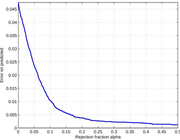
Figure 3: Error-reject curves (averaged over 10 runs) for different methods on the satimage task. Curve obtained by allowing the method to abstain from prediction on fractionαof test set, counting errors for predictions only. Depends on ranking of test points. Ranking score (over test points x∗): maxcPˆ(y∗=c|x∗)(mc-sep, mc-semi, mc-tied), maxcPˆc(+1|x∗) (1rest).
6.3 Flat Classification: Handwritten Digits
We use the USPS handwritten digits recognition task (LeCun et al., 1989). The covariates x are 16×16 gray-scale images with values in{16k+15|k=0, . . . ,30}. The task has n=7291 training, m=2007 test cases, and C=10 classes. No preprocessing was done.
We use Gaussian kernels (7) once more, different ones for each class. We do not optimize the 5-fold CV criterionΨusing the full training set, but subsets of size n0=2000. Our results are averaged over five runs with different randomly drawn training subsets for hyperparameter learning, while we use the full training set for final fitting. All optimizations are started from vc=10,wc=
(∑jVar[xj])−1=0.0166, and we setσ2=4 throughout. The parameters determining the running time are k1=25,k2=35,k3=40 during hyperparameter learning (on n0=2000 points), and k1=
0 0.05 0.1 0.15 0.2 0.25 0.3 0.35 0.4 0.45 0.5 0
0.005 0.01 0.015 0.02 0.025 0.03 0.035 0.04 0.045
Rejection fraction alpha
Error on predicted
Figure 4: Error-reject curves (averaged over 5 runs) for different methods on the USPS task. Curve obtained by allowing the method to abstain from prediction on fraction α of test set, counting errors for predictions only. Depends on ranking of test points.
Test errors are 4.77%(±0.18%). These results are state-of-the-art for kernel classification. Seeger (2003) reports 4.98% for the IVM (Sect. 4.8.4), where hyperparameters are learned auto-matically. Csat ´o (2002) states 5.15% for his sparse online method with multiple sweeps over the data (Sect. 5.2). Results for the support vector machine are given in Sch ¨olkopf and Smola (2002), Table 18.1, method SV-254, where a combination heuristic based on kernel PCA was used to attain a test error of 4.4%. Crammer and Singer (2001) quote a test error of 4.38%, kernel parameters having been selected by 5-fold cross-validation. All these used the Gaussian kernel as well. The latter studies do not quote fluctuations w.r.t. choices such as the fold partition in CV, which is not negligible in our case here. The SVM-based methods do not attempt test set rankings or predictive probability estimation, and the corresponding studies do not show error-reject (or ROC) curves. Seeger (2003) gives an error-reject curve, which is very similar to ours here.
after k2=80 LCG steps.17 Lessons learned from these large scale experiments are commented on in Section 4. There are delicate dependencies between k1,k2and the running time to convergence, which need to be explored in large scale settings, but this was not done thoroughly here.
7. Discussion
We have presented a general framework for learning kernel-based penalized likelihood classification methods from data. A central feature of the framework is its high computational efficiency, even though all classes are treated jointly. This is achieved by employing approximate Newton-Raphson optimization for the parameter fitting, which requires few large steps only for convergence. These steps are reduced to matrix-vector multiplication (MVM) primitives with kernel matrices. For gen-eral kernels, these MVM primitives can be reduced to large numerical linear algebra primitives, which can be computed very efficiently on modern computer architectures. This is very much in contrast to many chunking algorithms for kernel method fitting, which have been proposed in machine learning, and the advantages of our approach are detailed in Section 7.2. Dependencies between classes can be encoded a priori with minor additional efforts, as has been demonstrated for the case of hierarchical classification. Our method provides estimates of predictive probabilities which are asymptotically correct. Hyperparameters can be adjusted automatically, by optimizing a cross-validation log likelihood score in a gradient-based manner, and these computations are once more reduced to the same MVM primitives. This means that within our framework, all code opti-mization efforts can be concentrated on these essential primitives (see also Section 7.3), rather than having to tune a set of further heuristics.
7.1 Related Work
Our primary fitting optimization for flat multi-way classification appeared in Williams and Barber (1998), although some fairly essential features are novel here. They also did not consider large scale problems or class structures. Empirical Bayesian criteria such as the marginal likelihood are rou-tinely used for hyperparameter learning in Gaussian process models (Williams and Barber, 1998; Williams and Rasmussen, 1996). However, in cases other than regression estimation with Gaussian noise, the marginal likelihood for a GP model cannot be computed analytically, and approxima-tions differ strongly in terms of accuracy and computational complexity. For the multi-class model, Williams and Barber (1998) use an MAP approximation for fixed hyperparameters, just as we do, but their second-order approximation to the marginal likelihood is quite different from our criterion, conceptually as well as computationally (see below). Approximately solving large linear system by linear conjugate gradients (LCG) is standard in numerical mathematics, and has been used in machine learning as well (Gibbs, 1997; Williams and Barber, 1998; Keerthi and DeCoste, 2005).
The idea of optimizing approximations to a cross-validation score for hyperparameter learning is not novel (Craven and Wahba, 1979; Qi et al., 2004). Our approach is different to these, in that the CV score and gradient computations are reduced to elementary steps of the primary fitting method,
17. We cannot obtain a good initial α value from the finalα[Jk]of hyperparameter learning, because this is done on
so both can be done with the same code.18 In contrast, scores like GCV (Craven and Wahba, 1979) or second order marginal likelihood (Williams and Barber, 1998) come in terms of the form tr H−1 or log|H|for the Hessian H of size nC. There are approximate reductions of computing these terms to solving linear systems (randomized trace estimator, Lanczos), but they rely on additional sampling of Gaussian noise, which introduces significant inaccuracies. In practice, optimizing such “noisy” criteria is quite difficult, whereas our criterion can be optimized using standard optimization code. Qi et al. (2004) propose an interesting approach of approximating leave-one-out CV using expectation propagation, see also Opper and Winther (2000). They use a sparse approximation for efficiency, but they deal with a single-process model only (C=1), and it is not clear how to implement EP efficiently (scaling linearly in C) for the multi-class model. Interestingly, they observe that optimizing their approximate CV score is more robust to overfitting than the marginal likelihood. Finally, none of these papers propose (or achieve) a complete reduction to kernel MVM primitives only, nor do they deal with representing class structures or work on problems of the scale considered here.
Many different multi-class SVM techniques have been proposed, see Crammer and Singer (2001) and Hsu and Lin (2002) for references. These can be split into joint (“all-together”) and decomposition methods. The latter reduce the multi-class problem to a set of binary ones (“one-against-rest” of Section 6.2 is a prominent example), with the advantage that good code is available for the binary case. The problem with these methods is that the binary discriminants are fitted separately without knowledge of each other, or of their role in the final multi-way classifier, so in-formation from data is wasted. Also, their post-hoc combination into a multi-way discriminant is heuristic. Joint methods are like ours here, in that all classes are jointly represented. Fitting is a constrained convex problem, and often fairly sparse solutions (many zeros inα) are found. How-ever, in difficult structured label tasks, the degree of sparsity is usually not high, and in these cases, commonly used chunking algorithms for multi-class SVM can be very inefficient (see Section 7.2). We should note that our approach here cannot be applied directly to multi-class SVMs, since they require the solution of a constrained convex problem, but the principles used here should hold there as well. Some novel suggestions here appear independently in Keerthi et al. (2007). SVM methods typically do not come with efficient automatic kernel parameter learning schemes, and they do not provide estimates of predictive probabilities which are asymptotically correct.
On the other hand, in a direct comparison our implementation would still be slower than the highly optimized multi-class SVM code of Crammer and Singer (2001), at least on standard non-structured tasks such as USPS (Section 6.3) or MNIST. Especially on the latter, sparsity in α is clearly present, and years of experience with the SVM problem led to very effective ways of ex-ploiting it. In contrast,α in our approach is not sparse, and it is not our goal here to find a sparse approximation. Hyperparameters are selected “by hand” in their method, not via gradient-based op-timization. For a small number of hyperparameters, this traditional approach is often faster than our optimization-based one here, and importantly, it can be fully parallelized. However, our approach is still workable in situations with many dependent hyperparameters (for example, Section 7.4.1), where CV by hand simply cannot be done.
Our ANOVA setup for hierarchical classification is proposed by Cai and Hofmann (2004), whose use it within a SVM “all-together” method. We compare our method against theirs in
tion 6.1, achieving quite similar results in an order of magnitude less time. They also do not address the problem of hyperparameter learning.
7.2 Global versus Decomposition Methods
In most kernel methods proposed so far in machine learning, the primary fitting to data (for fixed hyperparameters) translates to a convex minimization problem, where the penalisation terms cor-respond to quadratic expressions with kernel matrices. While kernel matrices may show a rapidly decaying eigenvalue spectrum, they certainly do couple the optimization variables strongly.19 While a convex function can be optimized by any method which just guarantees descent in each step, there are huge differences in how fast the minimum is attained to a desired accuracy. In fact, in the ab-sence of local minima, the speed of convergence becomes the most important characteristic of a method, besides robustness and ease of implementation.
In machine learning, the most dominant technique for large scale (structured label) kernel clas-sification is what optimization researchers call block coordinate descent methods (BCD), see Bert-sekas (1999, Sect. 2.7). The idea is to minimize the objective w.r.t. a few variables at a time, keeping all others fixed, and to iterate this process using some scheduling over the variables. Each step is convex again,20 yet much smaller than the whole, and often the steps can be solved analytically. Ignoring the aspect of scheduling, such methods are simple to implement.
A complementary approach is to find search directions which lead to as fast a descent as possi-ble, these directions typically involve all degrees of freedom of the optimization variables. If local first and second order information can be computed, the optimal search direction is Newton’s, which has to be corrected if constraints are present (conditional gradient or gradient projection methods). If the Newton direction cannot be computed feasibly, approximations may be used. Such Newton-like methods are certainly vastly preferred in the optimization community, due to superior convergence rates, but also because features of modern computer architectures are used more efficiently, as is detailed below. In this paper, we advocate to follow this preference for kernel machine fitting in machine learning. We are encouraged not only by our own experiences, but can refer to the fact that (approximate) Newton methods are standard for fitting generalized linear models in statistics, and that such methods are also routinely used for Gaussian process models (Williams and Barber, 1998; Rasmussen and Williams, 2006), albeit typically on problems of smaller scale than treated here.
The dominance of BCD methods for kernel machine fitting, while somewhat surprising, can be attributed to early success stories with SVM training, culminating in the SMO algorithm (Platt, 1998), where only two variables are changed at a time. If an SVM is fitted to a task with low noise, the solution can be highly sparse, and if the active set of “support vectors” is detected early in the optimization process, methods like SMO can be very efficient. Importantly, SMO or other BCD methods are easily implemented. On the other hand, as SVMs are increasingly applied to hard structured label problems which usually do not have very sparse solutions, or whose active sets are hard to find, weaknesses of BCD methods become apparent.
Block coordinate descent methods are often referred to as using the “divide-and-conquer” prin-ciple, but this is not the case for kernel method fitting. BCD methods “are often useful in contexts where the cost function and the constraints have a partially decomposable structure with respect to
19. An almost low-rank kernel matrix translates into a coupling of a simple structure, but the dominant couplings are typically strong and not sparse.