A New Algorithm for Estimating the Effective Dimension-Reduction Subspace

(1)

A New Algorithm for Estimating

the Effective Dimension-Reduction Subspace

Arnak S. Dalalyan [email protected]

Universit´e Paris 6 - Pierre et Marie Curie Laboratoire de Probabilit´es, B. C. 188 75252 Paris Cedex 05, France

Anatoly Juditsky [email protected]

University Joseph Fourier of Grenoble LMC-IMAG 51 rue des Mathematiques, B. P. 53

38041 Grenoble Cedex 9, France

Vladimir Spokoiny [email protected]

Weierstrass Institute for Applied Analysis and Stochastics Mohrenstrasse 39, 10117 Berlin Germany

Editor: Aapo Hyvarinen

Abstract

The statistical problem of estimating the effective dimension-reduction (EDR) subspace in the multi-index regression model with deterministic design and additive noise is considered. A new procedure for recovering the directions of the EDR subspace is proposed. Many methods for estimating the EDR subspace perform principal component analysis on a family of vectors, say ˆ

β1, . . . ,βLˆ , nearly lying in the EDR subspace. This is in particular the case for the structure-adaptive approach proposed by Hristache et al. (2001a). In the present work, we propose to estimate the pro-jector onto the EDR subspace by the solution to the optimization problem

minimize max

`=1,...,L

ˆ

β>

`(I−A)β`ˆ subject to A∈Am∗,

whereAm∗ is the set of all symmetric matrices with eigenvalues in[0,1]and trace less than or equal to m∗, with m∗being the true structural dimension. Under mild assumptions,√n-consistency of the proposed procedure is proved (up to a logarithmic factor) in the case when the structural dimension is not larger than 4. Moreover, the stochastic error of the estimator of the projector onto the EDR subspace is shown to depend on L logarithmically. This enables us to use a large number of vectors ˆ

β`for estimating the EDR subspace. The empirical behavior of the algorithm is studied through numerical simulations.

Keywords: dimension-reduction, multi-index regression model, structure-adaptive approach,

cen-tral subspace

1. Introduction

One of the most challenging problems in modern statistics is to find efficient methods for treating high-dimensional data sets. In various practical situations the problem of predicting or explaining a scalar response variable Y by d scalar predictors X(1)_{, . . . ,}_X(d)_{arises. For solving this problem one}

(2)

between Y and X = (X(1), . . . ,X(d)), complex models are to be preferred. Unfortunately, the accu-racy of estimation is in general a decreasing function of the model complexity. For example, in the regression model with additive noise and two-times continuously differentiable regression function

f :Rd _→_R_{, the most accurate estimators of f based on a sample of size n have a quadratic risk} decreasing as n−4/(4+d)when n becomes large. This rate deteriorates very rapidly with increasing

d leading to unsatisfactory accuracy of estimation for moderate sample sizes. This phenomenon is

called “curse of dimensionality”, the latter term being coined by Bellman (1961).

To overcome the “curse of dimensionality”, additional restrictions on the candidates f for de-scribing the relationship between Y and X are necessary. One popular approach is to consider the multi-index model with m∗indices: for some linearly independent vectorsϑ1,. . .,ϑm∗and for some

function g :Rm∗ _→R_{, the relation f}₍_x_{) =}_g₍ϑ>

1x, . . . ,ϑ>m∗x) holds for every x∈Rd. Here and in

the sequel the vectors are understood as one column matrices and M> denotes the transpose of the matrix M. Of course, such a restriction is useful only if m∗<d and the main argument in favor

of using the multi-index model is that for most data sets the underlying structural dimension m∗is substantially smaller than d. Therefore, if the vectorsϑ1,. . .,ϑm∗ are known, the estimation of f

reduces to the estimation of g, which can be performed much better because of lower dimensionality of the function g compared to that of f .

Another advantage of the multi-index model is that it postulates that only few linear combina-tions of the predictors may suffice for “explaining” the response Y . Considering these combinacombina-tions as new predictors leads to a much simpler model (due to its low dimensionality), which can be suc-cessfully analyzed by graphical methods, see Cook and Weisberg (1999) and Cook (1998) for more details.

Throughout this work we assume that we are given n observations(Y1,X1), . . . ,(Yn,Xn)from the model

Yi= f(Xi) +εi=g(ϑ1>Xi, . . . ,ϑ>m∗Xi) +εi, (1)

whereε1, . . . ,εnare unobserved errors assumed to be mutually independent zero mean random vari-ables, independent of the design_{Xi,i≤n}.

Since it is unrealistic to assume thatϑ1, . . . ,ϑm∗ are known, estimation of these vectors from the

data is of high practical interest. When the function g is unspecified, only the linear subspace

S

_ϑ spanned by these vectors may be identified from the sample. This subspace is usually called index

space or dimension-reduction (DR) subspace. Clearly, there are many DR subspaces for a fixed

model f . Even if f is observed without error, only the smallest DR subspace, henceforth denoted by

S

, can be consistently identified. This smallest DR subspace, which is the intersection of all DR subspaces, is called effective dimension-reduction (EDR) subspace (Li, 1991) or central mean

subspace (Cook and Li, 2002). We adopt in this paper the former term, in order to be consistent

with Hristache et al. (2001a) and Xia et al. (2002), which are the closest references to our work. The present work is devoted to studying a new algorithm for estimating the EDR subspace. We call it structural adaptation via maximum minimization (SAMM). It can be regarded as a branch of the structure-adaptive (SA) approach introduced in Hristache et al. (2001b) and Hristache et al. (2001a).

(3)

the central mean subspace and to Cook and Ni (2005) for a discussion of the relationship between different algorithms estimating these subspaces.

There are a number of methods providing an estimator of the EDR subspace in our set-up. These include ordinary least square (Li and Duan, 1989), sliced inverse regression (Li, 1991), sliced inverse variance estimation (Cook and Weisberg, 1991), principal Hessian directions (Li, 1992), graphical regression (Cook, 1998), parametric inverse regression (Bura and Cook, 2001a), SA ap-proach (Hristache et al., 2001a), iterative Hessian transformation (Cook and Li, 2002), minimum average variance estimation (MAVE) (Xia et al., 2002), nonparametric linear smoothing for inverse regression (Bura, 2003), minimum discrepancy approach (Cook and Ni, 2005) marginal high mo-ment regression (Yin and Cook, 2006) density based MAVE and outer product of gradient (Xia, 2007), as well as the refinements using contour-projection (Wang et al., 2008), intraslice covariance estimation (Cook and Ni, 2006) and Lasso shrinkage (Ni et al., 2005; Li, 2007).

All these methods, except SA approach and MAVE, rely on the principle of inverse regression (IR). Therefore they inherit its well known limitations. First, they require a hypothesis on the prob-abilistic structure of the predictors usually called linearity condition. Second, there is no theoretical justification guaranteeing that these methods estimate the whole EDR subspace and not just a part thereof, see Cook and Li (2004, Section 3.1) and the comments on the third example in Hristache et al. (2001a, Section 4). In the same time, they have the advantage of being simple for implemen-tation and for inference.

The two other methods mentioned above—SA approach and MAVE—have much wider appli-cability including even time series analysis. The inference for these methods is more involved than that of IR based methods, but SA approach and MAVE need no strong requirements on the design of covariates or on the response variable. Moreover, in many cases they provide more accurate estimates of the EDR subspace (Hristache et al., 2001a; Xia et al., 2002; Xia, 2007).

These arguments, combined with empirical experience, indicate the complementarity of differ-ent methods designed to estimate the EDR subspace. It turns out that there is no procedure among those cited above that outperforms all the others in plausible settings. Therefore, a reasonable strat-egy for estimating the EDR subspace is to execute different procedures and to take a decision after comparing the obtained results. In the case of strong contradictions, collecting additional data is recommended.

The algorithm SAMM we introduce here exploits the fact that the gradient∇f of the regression

function f evaluated at any point x_∈Rd _{belongs to the EDR subspace. The estimation of the} gradient being an ill-posed inverse problem, it is better to estimate some linear combinations of

∇f(X1), . . . ,∇f(Xn), which still belong to the EDR subspace.

Let L be a positive integer. The main idea behind the algorithm proposed in Hristache et al. (2001a) consists in iteratively estimating L linear combinations β1, . . . ,βL of vectors∇f(X1), . . . ,

∇f(Xn)and then recovering the EDR subspace from the vectorsβ`by running a principal compo-nent analysis (PCA). The resulting estimator is proved to be√n-consistent provided that L is

cho-sen independently of the sample size n. Unfortunately, if L is small with respect to n, the subspace spanned by the vectorsβ1, . . . ,βLmay cover only a part of the EDR subspace. Therefore, empirical experience advocates for large values of L, even if the desirable feature of√n-consistency fails in

this case.

(4)

as the solution to a minimization problem involving a sum over L terms, see (5) in the next section, then, to some extent, our proposal consists in replacing the sum by the maximum. This motivates the term structural adaptation via maximum minimization. The main advantage of SAMM is that it allows us to deal with the case when L increases polynomially in n and yields an estimator of the EDR subspace which is consistent under a very weak identifiability assumption. In addition, SAMM provides a√n-consistent estimator (up to a logarithmic factor) of the EDR subspace when m∗_≤4.

If m∗=1, the corresponding model is referred to as single-index regression. There are many methods for estimating the EDR subspace in this case, see Yin and Cook (2005); Delecroix et al. (2006) and the references therein. Note also that the methods for estimating the EDR subspace have often their counterparts in the partially linear regression analysis, see for example Samarov et al. (2005) and Chan et al. (2004).

An interesting problem in the context of dimensionality reduction is the estimation of the true structural dimension m∗. Many approaches exist for constructing estimators of m∗, see (Li, 1991, Section 5), (Xia et al., 2002, Section 2.2), and Bura and Cook (2001b), Bura and Cook (2001a), Bura (2003) and Cook and Li (2004) and the references therein. Here we assume that the structural dimension is known, leaving the development of an extension to the case of unknown m∗for future investigation.

The rest of the paper is organized as follows. We review the structure-adaptive approach and introduce the SAMM procedure in Section 2. Theoretical features including√n-consistency of the

procedure are stated in Section 3. Section 4 contains an empirical study of the proposed procedure through Monte Carlo simulations. The technical proofs are deferred to Section 5.

2. Structural Adaptation and SAMM

Introduced in Hristache et al. (2001b), the structure-adaptive approach is based on two observa-tions. First, knowing the structural information helps better estimate the model function. Second, improved model estimation contributes to recovering more accurate structural information about the model. These advocate for the following iterative procedure. Start with the null structural infor-mation, then iterate the above-mentioned two steps (estimation of the model and extraction of the structure) several times improving the quality of model estimation and increasing the accuracy of structural information during the iteration.

2.1 Purely Nonparametric Local Linear Estimation

When no structural information is available, one can only proceed in a fully nonparametric way. A proper estimation method is based on local linear smoothing (cf. Fan and Gijbels, 1996, for more details): estimators of the function f and its gradient∇f at a point Xiare given by

ˆ

f(Xi) c

∇f(Xi) !

=arg min

(a,c)>

n

∑

j=1

Yj−a−c>Xi j 2

K _|Xi j|2/b2

=

_n

∑

j=1

1

Xi j

1

Xi j _>

K

|Xi j|2

b2

₋1 n

∑

j=1

Yj

1

Xi j

K

|Xi j|2

b2

,

(5)

with radius b centered at the point of estimation Xicontains at least d+1 design points. For large value of d this leads to a large bandwidth and to a strong estimation bias. The goal of the structural adaptation is to diminish this bias using an iterative procedure exploiting the available estimated structural information.

In order to transform these general observations into a concrete procedure, let us describe in the rest of this section how the knowledge of the structure can help to improve the quality of the estimation and how the structural information can be obtained when the function or its estimator is given.

2.2 Model Estimation When an Estimator of

S

is Available

Let us start with the case of known

S

. The function f has the same smoothness as g in the directions of the EDR subspace

S

spanned by the vectorsϑ1, . . . ,ϑm∗, whereas it is constant (and therefore,

infinitely smooth) in all the orthogonal directions. This suggests to apply an anisotropic bandwidth for estimating the model function and its gradient. The corresponding local-linear estimator can be defined by

ˆ

f(Xi) c

∇f(Xi) !

=

n

∑

j=1

1

Xi j

1

Xi j >

w∗_{i j}

−1 n

∑

j=1

Yj

1

Xi j

w∗_{i j} , (2)

with the weights w∗_{i j}=K(_|Π∗Xi j|2/h2), where h is some positive real number andΠ∗is the orthogo-nal projector onto the EDR subspace

S

. This choice of weights amounts to using infinite bandwidth in the directions lying in the orthogonal complement of the EDR subspace.

If only an estimator ˆA of the orthogonal projector Π∗ is available, a possible strategy is to replaceΠ∗ by ˆA in the definitions of the weights w∗_{i j}. This strategy is however too stringent, since it definitely discards the directions belonging to ˆ

S

⊥. Being not sure that our information about the structure is exact, it is preferable to define the neighborhoods in a softer way. This is done by setting

wi j=K(Xi j>(I+ρ−2Aˆ)Xi j/h2)and by redefining ˆ

f(Xi) c

∇f(Xi) !

=

_n

∑

j=1

1

Xi j

1

Xi j _>

wi j ₋1 n

∑

j=1

Yj

1

Xi j

wi j . (3)

Here,ρis a real number from the interval[0,1]measuring the importance attributed to the estimator ˆ

A. If we are very confident in our estimator ˆA, we should chooseρclose to zero.

2.3 Recovering the EDR Subspace from an Estimator of∇f

Suppose first that the values of the function ∇f at the points Xi are known. Then

S

is the linear subspace ofRd _{spanned by the vectors}∇_f₍_X

i), i=1, . . . ,n. For classifying the directions ofRd according to the variability of f in each direction and, as a by-product, identifying

S

, the principal component analysis (PCA) can be used.

Recall that the PCA method is based on the orthogonal decomposition of the matrix M ₌

n−1∑n_i₌₁∇f(Xi)∇f(Xi)>:M =OΛOT with an orthogonal matrix O and a diagonal matrixΛwith diagonal entriesλ1≥λ2≥. . .≥λd. Clearly, for the multi-index model with m∗-indices, only the first m∗ eigenvalues ofM _{are positive. The first m}∗ _{eigenvectors of}M _{(or, equivalently, the first}

(6)

Let L be a positive integer. In Hristache et al. (2001a), a “truncated” matrixM_L_{is considered,} which coincides withM _{if L equals n. Let}_{ψ_`_{, `}₌₁_{, . . . ,}_L_} _{be a set of vectors of}Rn_satisfying

the conditions n−1∑n_i₌₁ψ`,iψ`0_,i =δ_`,`0 for every `, `0∈ {1, . . . ,L}, with δ_`,`0 being the Kronecker

symbol. Define

β`=n−1 n

∑

i=1

∇f(Xi)ψ`,i (4)

andM_L₌∑L

`=1β`β>`. By the Bessel inequality, it holds MLM. Here and in the sequel, for two symmetric matrices A and B, AB means that B₋A is positive-semidefinite. Moreover, since

M M_L₌M_LM_{, any eigenvector of}M _{is an eigenvector of}M_L_{. Finally, by the Parseval equality,}

M_L₌M _{if L}₌_n.

The reason of considering the matrixM_L_{instead of}M _{is that}M_L_{can be estimated much better} than M_{. In fact, estimators of}M _{have poor performance for samples of moderate size because} of the sparsity of high dimensional data, ill-posedness of the gradient estimation and the non-linear dependence ofM _on∇_{f . On the other hand, estimation of}M_L_{reduces to the estimation of L linear} functionals of∇f and may be done with a better accuracy. The obvious limitation of this approach

is that it recovers the EDR subspace entirely only if the rank ofM_L_{coincides with the rank of}M_, which is equal to m∗. To enhance our chances of seeing the condition rank(M_L_{) =}_m∗_{fulfilled, we} have to choose L sufficiently large. In practice, L is chosen of the same order as n.

In the case when only an estimator of∇f is available, the above described method of recovering

the EDR directions from an estimator ofM_L _{has a risk of order} p_L_/_{n (Hristache et al., 2001a,} Theorem 5.1). This fact advocates against using very large values of L. We desire nevertheless to use many linear combinations in order to increase our chances of capturing the whole EDR subspace. To this end, we modify the method of extracting the structural information from the estimators ˆβ`of vectorsβ`.

Let m_≥m∗be an integer. Observe that the estimatorΠemof the projectorΠ∗based on the PCA solves the following quadratic optimization problem:

minimize

∑

`

ˆ

β>

`(I−Π)βˆ` subject to Π2=Π, trΠ≤m, (5) where the minimization is carried over the set of all symmetric (d_×d)-matrices. The value m∗ can be estimated by looking how many eigenvalues of Πem are significant. Let

Am

be the set of

(d_×d)-matrices defined as follows:

Am

=_{A : A=A>,0AI,tr A_≤m_}.

Define ˆAmas a minimizer of the maximum of the ˆβ>_`(I−A)βˆ`’s instead of their sum:

ˆ

Am∈arg min A∈Am

max `

ˆ

β>

`(I−A)βˆ`. (6)

(7)

3. Theoretical Features of SAMM

Throughout this section the true dimension m∗of the EDR subspace is assumed to be known. Thus, we are given n observations(Y1,X1), . . . ,(Yn,Xn)from the model

Yi= f(Xi) +εi=g(ϑ>1Xi, . . . ,ϑ>m∗Xi) +εi,

whereε1, . . . ,εn are independent centered random variables. The vectorsϑj are assumed to form an orthonormal basis of the EDR subspace entailing thus the representationΠ∗=∑m∗

j=1ϑjϑ>j. In what follows, we mainly consider deterministic design. Nevertheless, the results hold in the case of random design as well, provided that the errors are independent of X1, . . . ,Xn. Henceforth, without loss of generality we assume that_|Xi| ≤1 for any i=1, . . . ,n.

3.1 Description of the Algorithm

The structure-adaptive algorithm with maximum minimization consists of following steps.

a) Specify positive real numbers a_ρ, ah,ρ1and h1. Choose an integer L and select a set{ψ`, `≤

L_}of vectors fromRn_verifying_|ψ `|2=n. b) Set k=1 and ˆA0=0.

c) Define the estimators ∇cf_k(Xi) for i = 1, . . . ,n by formula (3) with

wi j=K Xi j>(I+ρk−2Aˆk−1)Xi j/h2k

. Set

ˆ

β`,k= 1

n

∑

i=1

c

∇f_k(Xi)ψ`,i, `=1, . . . ,L,

whereψ`,i is the ith coordinate ofψ`.

d) Define the new value ˆAkby ˆAk∈arg minA∈Am∗max` ˆ

β>

`,k(I−A)βˆ`,k. e) Setρk+1=aρ·ρk, hk+1=ah·hk and increase k by one.

f) Stop ifρk<ρminor hk>hmax, otherwise continue with the step c).

Let k(n)be the total number of iterations. We denote byΠbnthe orthogonal projection onto the space spanned by the eigenvectors of ˆAk(n)corresponding to the m∗largest eigenvalues. The estimator of

the EDR subspace is then the image ofΠbn.

Both ˆAk(n)andΠbn are estimators of the projector onto

S

. Our theoretical results are stated for the estimatorΠbn, but similar results are valid for ˆAk(n), too. The numerical simulations we made

showed that these two estimators have comparable performances.

The described algorithm requires the specification of the parametersρ1, h1, aρand ah, as well as the choice of the set of vectors_{ψ`}. In what follows we use the values

ρ1=1, ρmin=n−1/(3∨m

∗₎

, aρ=e−1/2(3∨m∗), h1=C0n−1/(4∨d), hmax=2

√

d, ah=e1/2(4∨d).

(8)

the bias and the variance of estimation. The constant C0 will be chosen in a design-dependent manner taking into account the fact that the local neighborhoods used in (2) should contain enough design points to entail the consistency of the estimator. The choice of L and that of vectorsψ` will be discussed in Section 4.

3.2 Assumptions

Prior to stating rigorous theoretical results we need to introduce a set of assumptions. From now on, we use the notation I for the identity matrix of dimension d,_kA_k2for the largest eigenvalue of A>A

and_kA_k2for the Frobenius norm of A (square root of the sum of squares of elements of A).

We start with the smoothness assumption ensuring the adequacy of the local linear approxima-tion of the regression funcapproxima-tion.

(A1) There exists a positive real Cg such that|∇g(x)| ≤Cg and|g(x)−g(x0)−(x−x0)>∇g(x)| ≤

Cg|x−x0|2for every x,x0∈Rm

∗

.

Unlike the smoothness assumption, the assumptions on the identifiability of the model and the regularity of design are more involved and specific to our algorithm. The formal statements read as follows.

(A2) Let the vectorsβ`∈Rdbe defined by (4) and let

B

∗=β¯=∑L`=1c`β`:∑`L=1|c`| ≤1 . There exist vectors ¯β1, . . . ,β¯m∗∈

B

∗and constants µ₁, . . . ,µ_m∗ such that

Π∗ m

∗

∑

k=1

µkβ¯kβ¯>k. (7)

We denote µ∗=µ1+. . .+µm∗.

Remark 1 Assumption (A2) implies that the subspace

S

=Im(Π∗₎ _{is the smallest DR subspace,} therefore it is the EDR subspace. Indeed, for any DR subspace

S

0, the gradient∇f(Xi) belongs

to

S

0 for every i. Therefore β` ∈

S

0 for every `≤L and

B

∗ ⊂

S

0. Thus, for every β◦ from the

orthogonal complement

S

0⊥, it holds|Π∗_β◦_|2_≤_∑

kµk|β¯>kβ◦|2=0. Therefore

S

0⊥⊂

S

⊥ implying

thus the inclusion

S

_⊂

S

0.

Lemma 2 If the family{ψ`}spansRn, then assumption (A2) is always satisfied with some µk(that

may depend on n).

Proof SetΨ= (ψ1, . . . ,ψL)∈Rn×L,∇f= (∇f(X1), . . . ,∇f(Xn))∈Rd×nand write the d×L matrix

B= (β1, . . . ,βL)in the form∇f·Ψ. Recall that if M1,M2are two matrices such that M1·M2is well defined and the rank of M2coincides with the number of lines in M2, then rank(M1·M2) =rank(M1). This implies that rank(B) =m∗provided that rank(Ψ) =n, which amounts to span(_{ψ`}) =Rn.

Let now ˜β1, . . . ,β˜m∗ be a linearly independent subfamily of{β_`, `≤L}. Then the m∗th largest

eigenvalueλm∗(M˜)of the matrix M˜ =∑_km₌∗₁β˜_kβ˜>_k is strictly positive. Moreover, if v₁, . . . ,v_m∗ are

the eigenvectors of M˜ _{corresponding to the eigenvalues}λ₁₍M˜₎_≥_{. . .}_≥λ_m∗(M˜)>0, then

Π∗₌ m

∗

∑

k=1

vkv>k 1

λm∗(M˜)

m∗

∑

k=1

λk(M˜)vkv>k =λm∗(M˜)−1M˜ =λ_m∗(M˜)−1

m∗

∑

k=1 ˜

(9)

Hence, inequality (7) is fulfilled with µk=λm∗(M˜)−1for every k=1, . . . ,m∗.

These arguments show that the identifiability assumption (A2) is fairly weak. In fact, since we always choose_{ψ`}so that span({ψ`}) =Rn, (A2) amounts to requiring that the value µ∗remains bounded when n increases. This assumption is much weaker than the coverage assumption under which the consistency of the inverse regression based methods is proved.

Let us proceed with the assumption on the design regularity. Define P₁∗ =I and P_k∗= (I+

ρ−2

k Π∗)−1/2for every k≥2. Next, set Z

(k)

i j = (hkPk∗)−1Xi jand for any d×d matrix U put w(i jk)(U) =

K (Z_{i j}(k))>U Z_{i j}(k), ¯w(_{i j}k)(U) =K0 (Z(_{i j}k))>U Z_{i j}(k), N_i(k)(U) =∑jw

(k)

i j (U)and

V_i(k)(U) =

n

∑

j=1

1

Z_{i j}(k)

1

Z_{i j}(k)

>

w(_{i j}k)(U).

(A3) For some positive constants CV,CK,CK0,C_wand for someα∈]0,1/2], the inequalities

kV_i(k)(U)−1_kN_i(k)(U)_≤CV, i=1, . . . ,n, n

∑

i=1

w(_{i j}k)(U)/N_i(k)(U)_≤CK, j=1, . . . ,n,

n

∑

i=1

|w¯(_{i j}k)(U)_|/N_i(k)(U)_≤CK0, j=1, . . . ,n,

n

∑

j=1

|w¯(_{i j}k)(U)_|/N_i(k)(U)_≤Cw i=1, . . . ,n,

hold for every k_≤k(n)and for every d_×d matrix U verifying_kU₋I_k2≤α.

Remark 3 Note that in (A3) we implicitly assumed that the matrices V_i(k)are invertible, which may be true only if any neighborhood E(k)(Xi) ={x :|(I+ρ_k−2Π∗)−1/2(Xi−x)| ≤hk}contains at least

d design points different from Xi. The parameters h1,ρ1, aρand ah are chosen so that the volume

of ellipsoids E(k)(Xi)is a non-decreasing function of k and Vol(E(1)(Xi)) =C0/n. Therefore, from

theoretical point of view, if the design is random with positive density on[0,1]d_{, it is easy to check}

that for a properly chosen constant C0, assumption (A3) is satisfied with a probability close to one.

In applications, we define h1as the smallest real such that mini=1,...,n#E(1)(Xi) =d+1 and add to

the matrix

n

∑

j=1

1

Xi j

1

Xi j _>

wi j,

involved in the definition (3), a small full-rank matrix to be sure that the resulting matrix is invertible, see Section 4. This observation also implies that the SAMM procedure can not be applied in the case where the sample size n is smaller than or equal to the dimension d of predictors.

(10)

3.3 Risk Bounds for the Projection Matrix Estimation

In this section, we present the main result of the paper assessing the quality of the estimator Πbn of the projection matrixΠ∗ in the asymptotics of large samples. To this end, we assume that the kernel K used in (3) is chosen to be continuous, positive and vanishing outside the interval[0,1]. The vectorsψ`are assumed to verify

max

`=1,...,Li=max1,...,n|ψ`,i|<ψ,¯ (8) for some constant ¯ψindependent of n. In the sequel, we denote by C,C1, . . .some constants depend-ing only on m∗,µ∗,Cg,CV,CK,CK0,C_wand ¯ψ.

Theorem 4 Let assumptions (A1)-(A4) be fulfilled. There exists C >0 such that for any z_∈

]0,2plog(nL)]and for sufficiently large values of n, it holds

P q

tr(I₋Πbn)Π∗>Cn−

2 3∨m∗t2

n+

2√µ∗zc0σ p

n(1₋ζn)

≤Lze−z22−1+3k(n)−5

n ,

where c0=ψ¯√dCKCV, tn=O( p

log(Ln))andζn=O(tnn−

1 6∨m∗).

Corollary 5 Under the assumptions of Theorem 4, for sufficiently large n, it holds P

kΠbn−Π∗k2>Cn−

2 3∨m∗t2

n+

2√2µ∗zc0σ p

n(1₋ζn)

≤Lze−z22−1+3k(n)−5 n

E(_kΠbn−Π∗k2)≤C

n−3∨2m∗t2 n+

√

log nL

√_n

+

√

2m∗₍_3k₍_n₎₋₅₎

n .

Proof Easy algebra yields

kΠbn−Π∗k22=tr(Πbn−Π∗)2=trΠb2n−2 trΠbnΠ∗+trΠ∗ ≤trΠbn+m∗−2 trΠbnΠ∗≤2m∗−2 trΠbnΠ∗.

The equality trΠ∗=m∗ and the linearity of the trace operator complete the proof of the first in-equality. The second inequality can be derived from the first one by standard arguments in view of the inequality_kΠbn−Π∗k2₂≤2m∗.

According to these results, for m∗_≤4, the estimator of the orthogonal projector onto

S

provided by the SAMM procedure is√n-consistent up to a logarithmic factor. This rate of convergence is

known to be optimal for a broad class of semiparametric problems, see Bickel et al. (1998) for a detailed account on the subject.

Remark 6 The inspection of the proof of Theorem 4 shows that the factor t_n2multiplying the “bias” term n−2/(3∨m∗)disappears when m∗>3.

Remark 7 The same rate of convergence remains valid in the case when the errors are not

(11)

3.4 Risk Bound for the Estimator of a Basis of the EDR Subspace

The main result of this paper stated in the preceding subsection provides a risk bound for the esti-matorΠbn ofΠ∗, the orthogonal projector onto

S

. As a by-product of this result, we show in this section that a similar risk bound holds also for the estimator of an orthonormal basis of

S

. This means that for an arbitrarily chosen orthonormal basis of the estimated EDR subspace ˆ

S

=Im(Πbn), there is an orthonormal basis of the true EDR subspace

S

such that the matrices built from these bases are close in Frobenius norm with a probability tending to one.

Proposition 8 Let the assumptions of Theorem 4 be fulfilled. For any orthonormal basis ˆϑ1, . . . ,ϑˆm∗ of the estimated EDR subspace ˆ

S

=Im(Πbn)there exists an orthonormal basisϑ1, . . . ,ϑm∗of the true EDR subspace

S

=Im(Π∗)such that, for sufficiently large n, it holds

P

kΘbn−Θk2>Cn−

2 3∨m∗t2

n+

2(√m∗₊₁₎√_2µ∗_zc₀σ

p

n(1₋ζn)

≤Lze−z22−1+3k(n)−5

n ,

whereΘbn(resp.Θ) is the d×m∗matrix whose jth column is ˆϑj(resp.ϑj).

Proof Using the singular value decomposition, we write Π∗Θbn =UΛV>, where U and V are orthogonal matrices andΛ is a diagonal matrix. Let us denote by λj, uj, vj respectively the jth diagonal entry ofΛ, the jth column of U and the jth column of V . SinceΠ∗Θbnvj =λjuj, we have

λj=|λjuj|=|Π∗Θbnvj| ≤1. On the other hand,

λj=|Π∗Θbnvj| ≥ |Θbnvj| − |(Πbn−Π∗)Θbnvj| ≥1− kΠbn−Π∗k,

where we used the fact that_|Θbnvj|2=v>jΘbn>Θbnvj=v>jvj=1. Let us define the matrixΘas follows:

Θ=U Id×m∗V>, where I_d_×_m∗ is the d×m∗diagonal matrix with all diagonal entries equal to one.

One easily checks thatΘis orthogonal, that isΘ>Θ=Im∗. Moreover, we haveΘ=Π∗Θˆ_nVΛ−V>,

whereΛ− is the m∗_×m∗ diagonal matrix havingλ−_j1 as jth diagonal entry. Note that if the norm of ˆΠn−Π∗ is less than 1, the eigenvaluesλj are strictly positive. In this case,Λ− is well defined and we obviously haveΠ∗Θ=Θ. Thus the columns ofΘ form an orthonormal basis of Im(Π∗₎_.

Furthermore, we have

kΘbn−Θk2≤ kΘ−Π∗Θbnk2+k(Π∗−Πbn)Θk2 ≤ kU(Id×m∗−Λ)V>k2+kΠ∗−Πbnk2 ≤(

m∗

∑

j=1

(λj−1)2)1/2+kΠ∗−Πbnk2 ≤(√m∗₊₁₎_kΠ∗₋_Π_b

nk2,

(12)

4. Simulation Results

The aim of this section is to demonstrate on several examples how the performance of the algorithm SAMM depends on the sample size n, the dimension d and the noise levelσ. We also show that our procedure can be successfully applied in autoregressive models. Many unreported results show that in most situations the performance of SAMM is comparable to the performance of SA approach based on PCA and to that of MAVE. A thorough comparison of the numerical virtues of these methods being out of scope of this paper, we simply show on some examples that SAMM may substantially outperform MAVE in the case of large “bias”. Our results also show that SAMM and MAVE provide more accurate estimates of the EDR subspace than inverse regression based methods : inverse regression based on Minimum Discrepancy Approach (MDA) introduced in Cook and Ni (2005) and Sliced Average Variance Estimation (SAVE) of Cook and Weisberg (1991). In all simulations for inverse regression based methods, the number of slices is chosen to minimise the risk.

The computer code of the procedure SAMM is distributed freely, it can be downloaded from

http://code.google.com/p/samm07/. It requires the MATLAB packages SDPT3 and YALMIP.

We are grateful to Professor Yingcun Xia for making the computer code of MAVE available to us. To obtain higher stability of the algorithm, we preliminarily standardize the response Y and the predictors X(j). More precisely, we deal with ˜Yi=Yi/σY and ˜X =diag(ΣX)−1/2X , whereσY2 is the empirical variance of Y ,ΣX is the empirical covariance matrix of X and diag(ΣX)is the d×d matrix obtained fromΣX by replacing the off-diagonal elements by zero. To preserve consistency, we set

˜

β`,k(n)=diag(ΣX)−1/2βˆ`,k(n), where ˆβ`,k(n) is the last-step estimate of β`, and define Πbk(n) as the

solution to (6) with ˆβ`replaced by ˜β`,k(n). Furthermore, we add the small full-rank matrix Id+1/n to

∑n j=1

1 Xi j

>

wi jin (3).

In all examples presented below the number of replications is N =250; for each replication, a new sample of the design and the error vector(ε1, . . . ,εn) has been generated at random. The mean loss erN= _N1∑jerj and the standard deviation

q 1

N∑j(erj−erN)2 are reported, where erj= kΠb(j)₋_Π∗_k_with_Π_b(j)_{being the estimator of}_Π∗_{for jth replication.}

4.1 Choice of_{ψ`, `≤L}

The set_{ψ`}plays an essential role in the algorithm. The optimal choice of this set is an important issue that needs further investigation. We content ourselves with giving one particular choice which agrees with theory and leads to nice empirical results.

Let S_j_{, j}_≤_{d, be the permutation of the set} _{₁_{, . . . ,}_n_} _{satisfying X}(j)

S_j(1)≤. . .≤X (j)

S_j(n). Let

S−1

j be the inverse ofSj, that is,Sj(S− 1

j (k)) =k for every k=1, . . . ,n. Define{ψ`}as the set of vectors

(

cos 2π(k−1)S

−1

j (1) n

, . . . ,cos 2π(k−1)S

−1

j (n) n

>

sin 2πkS

−1

j (1) n

, . . . ,sin 2πkS

−1

j (n) n

> ,k≤[n/2], j≤d

)

normalized to satisfy∑n_i₌₁ψ2

`,i=n for every`. It is easily seen that these vectors satisfy conditions (8) and span(_{ψ`}) =Rn, so the conclusion of Lemma 2 holds. Above,[n/2]is the integer part of

(13)

The idea behind the above described choice of vectors ψ` is the following: if the design is uniformly distributed in[0,1]d _{and H}₍_x₎_{is a function}_Rd_→_R_{depending only on one coordinate} of x, the projections of the vector g= (H(X1), . . . ,H(Xn))> on some of directions ψ` are nearly equal to the Fourier coefficients of H. Indeed, for n odd and for every fixed j, the vectors{ek,j=

φk(S−j1(1)/n),φk(S−j1(2)/n), . . . ,φk(S−j1(n)/n) _>

; 1_≤k_≤n_}with_{φk}being the trigonometric basis (that is φ2p(x) =

√

2 sin(2πpx) andφ2p+1(x) = √

2 cos(2πpx) for every p_∈N_{) form an}

or-thonormal basis ofRn_{. Therefore, for any function H from}_Rd_to_R_{, which depends exclusively on} the jthcoordinate x(j)of x, one has g>ek j=∑ni=1H0(Xi(j))φk(S−j1(i)/n) =∑in=1H0(XS(j_j)(i))φk(i/n) for some function H0 :R→ R. Since for a sample X(

j)

1 , . . . ,X

(j)

n drawn from uniform distribu-tion in[0,1]the order statistics are nearly equal to i/n, we get 1_ng>ek j≈ 1_n∑ni=1H0(i/n)φk(i/n)≈ hH0,φkiL2_[_0,1_]. Note that although this explanation is valid only for uniform design and a function H depending only on one coordinate, empirical results show that this choice leads to satisfactory

results in more general situations.

4.2 Example 1 (Single-index) We set d=5 and f(x) =g(ϑ>_x₎_with

g(t) =4_|t_|1/2sin2(πt), and ϑ= (1/√5,2/√5,0,0,0)>_∈R5_.

We ran SAMM, MAVE, MDA and SAVE procedures on the data generated by the model

Yi= f(Xi) +0.5·εi,

where the design X is such that the coordinates(X_i(j),j_≤5,i_≤n)are i.i.d. uniform in[₋1,1], and the errorsεiare i.i.d. standard Gaussian independent of the design.

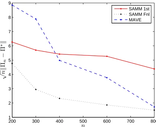
Table 1 contains the average loss for different values of the sample size n for the first step estimator by SAMM, the final estimator provided by SAMM and the estimators based on MAVE, MDA and SAVE. The first observation is that inverse regression based methods are not consistent in this case. We plot in Figure 1 the average loss normalized by the square root of the sample size n versus n. It is clearly seen that the iterative procedure improves considerably the quality of estimation and that the final estimator provided by SAMM is √n-consistent. In this example,

MAVE method often fails to recover the EDR subspace. However, the number of failures decreases very rapidly with increasing n. This is the reason why the curve corresponding to MAVE in Figure 1 decreases with a strong slope.

4.3 Example 2 (Double-index) For d_≥2 we set f(x) =g(ϑ>x)with

g(x) = (x1−x23)(x13+x2);

and ϑ1= (1,0, . . . ,0)∈Rd, ϑ2= (0,1, . . . ,0)∈Rd. We ran SAMM, MAVE, MDA and SAVE

procedures on the data generated by the model

(14)

200 300 400 500 600 700 800 1

2 3 4 5 6 7 8 9

n √ n

k

bΠn

−

Π

∗k

SAMM 1st SAMM Fnl MAVE

Figure 1: Average loss multiplied by√n versus n for the first step (solid line) and the final (dotted

line) estimators provided by SAMM and for the estimator by MAVE (dashed line) in Example 1.

n 200 300 400 600 800

SAMM, 1st 0.443 0.329 0.271 0.215 0.155 (.211) (.120) (.115) (.095) (.079) SAMM, Fnl 0.337 0.170 0.116 0.076 0.053 (.273) (.147) (.104) (.054) (.031)

MAVE 0.626 0.455 0.249 0.154 0.061

(.363) (.408) (.342) (.290) (.161)

MDA 0.882 0.885 0.890 0.885 0.882

(.144) (.141) (.130) (.142) (.148)

SAVE 0.857 0.847 0.832 0.818 0.782

(.145) (.144) (.154) (.168) (.169)

Table 1: Average loss _kΠb₋Π∗_kof the estimators obtained by SAMM, MAVE, MDA and SAVE procedures in Example 1. The standard deviation is given in parentheses.

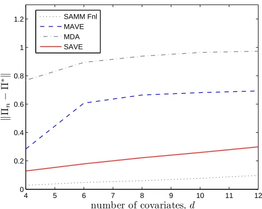
where the design X is such that the coordinates(X_i(j),j≤d,i≤n)are i.i.d. uniform in[₋40,40], and the errorsεi are i.i.d. standard Gaussian independent of the design. The results of simulations for different values of d are reported in Table 2.

(15)

4 5 6 7 8 9 10 11 12 0

0.2 0.4 0.6 0.8 1 1.2

number of covariates,d

k

bΠn

−

Π

∗k

SAMM Fnl MAVE MDA SAVE

Figure 2: Average loss versus d for the estimators provided by SAMM (dotted line), by MAVE (dashed line), by MDA (dash-dot line) and by SAVE (solid line) in Example 2.

d 4 6 8 10 12

SAMM 1st 0.154 0.242 0.296 0.365 0.421 (.063) (.081) (.071) (.087) (.095) SAMM, Fnl 0.028 0.048 0.060 0.077 0.098 (.011) (.020) (.021) (.026) (.037)

MAVE 0.284 0.607 0.664 0.681 0.693

(.147) (.073) (.052) (.054) (.044)

MDA 0.768 0.894 0.938 0.964 0.973

(.232) (.142) (.095) (.062) (.049)

SAVE 0.129 0.179 0.222 0.259 0.299

(.048) (.047) (.050) (.058) (.071)

Table 2: Average loss_kΠb₋Π∗_kof the estimators obtained by SAMM, MAVE and MDA procedures in Example 2. The standard deviation is given in parentheses.

4.4 Example 3

For d=5 we set f(x) =g(ϑ>_x₎_with

g(x) = (1+x1)(1+x2)(1+x3)

andϑ1= (1,0,0,0,0), ϑ2 = (0,1,0,0,0),ϑ3= (0,0,1,0,0). We ran SAMM, MAVE, MDA and SAVE procedures on the data generated by the model

(16)

σ 200 150 100 50 25 10 SAMM 1st 0.227 0.177 0.141 0.119 0.113 0.106 (.092) (.075) (.055) (.051) (.048) (.043) SAMM, Fnl 0.125 0.084 0.057 0.039 0.034 0.030 (.076) (.037) (.026) (.019) (.021) (.018)

MAVE 0.103 0.087 0.073 0.062 0.063 0.059

(.041) (.035) (.027) (.023) (.024) (.023)

MDA 0.854 0.850 0.867 0.862 0.858 0.873

(.167) (.173) (.157) (.159) (.171) (.159)

SAVE 0.510 0.511 0.496 0.505 0.496 0.490

(.208) (.204) (.207) (.197) (.196) (.199)

Table 3: Average losskΠb−Π∗_k _{of the estimators obtained by SAMM and MAVE procedures in}

Example 3. The standard deviation is given in parentheses.

where the design X is such that the coordinates(X_i(j),j_≤d,i_≤n)are i.i.d. uniform in[0,20], and the errorsεiare i.i.d. standard Gaussian independent of the design.

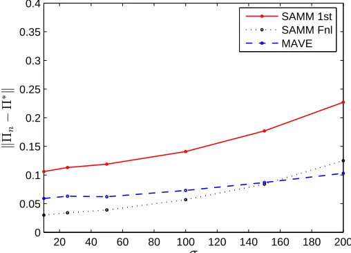
Figure 3 shows that the qualities of both SAMM and MAVE deteriorate linearly in σ, when

σincreases. These results also demonstrate that, thanks to an efficient bias reduction, the SAMM procedure outperforms MAVE when stochastic error is small, whereas MAVE works better than SAMM in the case of dominating stochastic error (that is whenσis large).

20 40 60 80 100 120 140 160 180 200

0 0.05 0.1 0.15 0.2 0.25 0.3 0.35 0.4

σ

k

bΠn

−

Π

∗ k

SAMM 1st SAMM Fnl MAVE

(17)

4.5 Example 4 (Time Series)

Let now T1, . . . ,Tn+6be generated by the autoregressive model

Ti+6= f(Ti+5,Ti+4,Ti+3,Ti+2,Ti+1,Ti) +0.2·εi, i=1, . . . ,n,

with initial variables T1, . . . ,T6being independent standard normal independent of the innovations

εi, which are i.i.d. standard normal as well. Let now f(x) =g(ϑ>x)with

g(x) =₋1+0.6x1−cos(0.5πx2) +e−x

2 3,

and

ϑ1= (1,0,0,2,0,0)/ √

5, ϑ2= (0,0,1,0,0,2)/

√

5, ϑ3= (−2,2,−2,1,−1,1)/

√

15.

We ran SAMM and MAVE procedures on the data (Xi,Yi), i=1, . . . ,250, where Yi =Ti+6 and

Xi= (Ti, . . . ,Ti+5)>. The results of simulations reported in Table 4 show that the qualities of SAMM and MAVE are comparable, with SAMM being slightly better. SAVE is better than MDA, but both of them are far less accurate than SAMM and MAVE.

n 300 400 500 600

SAMM, 1st 0.391 0.351 0.334 0.293 (.172) (.161) (.137) (.132) SAMM, Fnl 0.220 0.186 0.174 0.146 (.119) (.123) (.102) (.089)

MAVE 0.268 0.231 0.209 0.182

(.209) (.170) (.159) (.122)

MDA 0.914 0.915 0.913 0.912

(.115) (.107) (.119) (.119)

SAVE 0.617 0.515 0.428 0.369

(.200) (.184) (.151) (.138)

Table 4: Average loss _kΠb₋Π∗_kof the estimators obtained by SAMM, MAVE, MDA and SAVE procedures in Example 4. The standard deviation is given in parentheses.

5. Proofs

(18)

5.1 One Step Improvement

Let{δk}be a sequence of positive numbers to be chosen later and letPk=

A∈

Am

∗: tr(I−A)Π∗≤ δ2

k . Recall that we use the following notation:

P_k∗= (I+ρ−_k2Π∗)−1/2, Z_{i j}(k)= (hkPk∗)−1Xi j, w(_{i j}k)(U) =K (Z(_{i j}k))>U Z_{i j}(k)

N_i(k)(U) =

∑

j

w(_{i j}k)(U), V_i(k)(U) =

n

∑

j=1

1

Z_{i j}(k)

1

Z(_{i j}k)

>

w(_{i j}k)(U),

where U is a d_×d symmetric positive-semidefinite matrix. Let us define Sk= (I+ρ_k−2Aˆk−1)1/2and

Uk=Pk∗S2kPk∗.

One easily checks that the estimator∇cf_k(Xi)is given by ˆ

fk(Xi) c

∇f_k(Xi) !

=n

n

∑

j=1

1

Xi j

1

Xi j >

w(_{i j}k)(Uk) o−1 n

∑

j=1

Yj

1

Xi j

w(_{i j}k)(Uk),

Simple algebra yields

h−_k1fˆk(Xi)

P_k∗∇cf_k(Xi) !

=h−_k1V_i(k)(Uk)−1 n

∑

j=1

Yj

1

Z(_{i j}k)

w(_{i j}k)(Uk).

In order to study the behavior of∇cf_k, we will proceed in a first step as if Ukwere deterministic. For this reason, the notation

h−_k1f¯k(Xi)

P_k∗∇f_k(Xi) !

=h−_k1V_i(k)(Uk)−1 n

∑

j=1

f(Xj)

1

Z_{i j}(k)

w(_{i j}k)(Uk),

will be useful. In fact,∇f_k(Xi)defined as above would be the expectation of∇cfk(Xi)if Uk were deterministic.

Proposition 9 Let assumptions (A1)-(A4) be fulfilled. If for some integer k ∈[2,k(n)] the real numberαk=2δ2_k₋₁ρ_k−2+2δk₋1ρ−_k1is less than the constantαappearing in assumption (A3), then

there exist Gaussian vectorsξ∗_1,k, . . . ,ξ∗_L,k_∈Rd_{such that max}₁_≤_`_≤_L_E_[_|ξ∗

`,k|2]≤c20σ2and P

max 1_≤`≤L

P_k∗(βˆ`,k−β`)−

ξ∗

`,k √_{n h}

k

≥ϒk,Aˆk−1∈Pk−1

≤ 2_n ,

where we used the notationϒk= √

CVCg(ρk+δk−1)2hk+c1σαktn/(√n hk)with tn=4+(3 log(Ln)+ 3

2d2log n)1/2, c0=ψ¯(dCKCV)1/2and c1=15 ¯ψ(Cw2CV4CK2+CV2CK20)1/2.

Proof Let us start with evaluating the “bias” term_|P_k∗(β¯`,k−β`)|, where the vectors ¯β`,kare defined as 1_n∑n_i₌₁∇f_k(Xi)ψ`,i. According to the Cauchy-Schwarz inequality, it holds

P_k∗ β¯`,k−β`2=n−2 n

∑

i=1

P_k∗ ∇f_k(Xi)−∇f(Xi) _ψ `,i 2

≤n−2

n

∑

i=1

P_k∗ ∇f_k(Xi)−∇f(Xi) 2 n

∑

i=1

ψ2 l,i

≤ max i=1,...,n

P_k∗ ∇f_k(Xi)−∇f(Xi) 2

(19)

Simple computations show that

P_k∗ ∇f_k(Xi)−∇f(Xi)≤

h−_k1f¯k(Xi)

P_k∗∇f_k(Xi) !

− h

−1 k f(Xi)

P_k∗∇f(Xi) ! = h− 1 k V

(k)

i (Uk)−1 n

∑

j=1

f(Xj)

1

Z_{i j}(k)

w(_{i j}k)(Uk)−

h−_k1f(Xi)

P_k∗∇f(Xi) !

=h−_k1

V_i(k)(Uk)−1 n

∑

j=1

ri j

1

Z_{i j}(k)

w(_{i j}k)(Uk)

:=b(Xi),

where ri j = f(Xj)− f(Xi)−Xi j>∇f(Xi). Define vj = Vi(k)(Uk)−1/2

1

Z_{i j}(k)

q

w(_{i j}k)(Uk), λj =

h−_k1ri j q

w(_{i j}k)(Uk)andλ= (λ1, . . . ,λn)>. Then∑jvjv>j =Id+1and

b(Xi) =

Vi(k)(Uk)−1/2 n

∑

j=1

λjvj ≤

V_i(k)(Uk)−1/2 _{· |}λ|.

Note now that in view of Lemma 21,_kUk−Ik2≤αkon the event{Aˆk−1∈Pk−1}. Therefore,

b(Xi)2≤h−_k2

V_i(k)(Uk)−1/2 2·

n

∑

j=1

r2_{i j}w(_{i j}k)(Uk)

≤h−_k2 max j:w(i jk)(Uk)6=0

r2_{i j}

V_i(k)(Uk)−1 ·

n

∑

j=1

w(_{i j}k)(Uk)≤CVh−_k2 max j:w(i jk)(Uk)6=0

r_{i j}2.

Let us denote byΘthe(d_×m∗)matrix havingϑl as lth column. ThenΠ∗=ΘΘ>and therefore, in view of (A1),

|ri j|=|f(Xj)−f(Xi)−Xi j>∇f(Xi)|

=_|g(Θ>Xj)−g(Θ>Xi)−(Θ>Xi j)>∇g(Θ>Xi)| ≤Cg|Θ>Xi j|2=Cg|Π∗Xi j|2.

Since the weights w(_{i j}k)are defined via the kernel function K vanishing on the interval[1,∞[, we have max

j:w(i jk)(Uk)6=0

r2_{i j} =max_{r2_{i j} :_|SkXi j| ≤hk}. By Corollary 19, the inequality |SkXi j| ≤hk implies |Π∗Xi j| ≤(ρk+δk₋1)hk. On the other hand, |Π∗Xi j| ≤ |Xi j| ≤ |SkXi j| ≤hk. These estimates yield |b(Xi)| ≤√CVCg{(ρk+δk−1)∧1}2hk, and consequently,

max `=1,...,L

P_k∗ β¯`,k−β`≤max

i b(Xi)≤ p

CVCg{(ρk+δk₋1)∧1}2hk. (9) Let us evaluate now the “stochastic” error P_k∗ βˆ`,k−β¯`,k. Define E1as the d×(d+1)matrix(0 I), where 0 stands for the vector all coordinates of which are zero and I is the d_×d identity matrix.

Using this notation, we have P_k∗ βˆ`,k−β¯`,k

=∑n

j=1cj,`(Uk)εj, where

cj,`(Uk) = 1

nhk n

∑

i=1

E1Vi(k)(Uk)−1

1

Z_{i j}(k)

(20)

Let us defineξ∗_`,k=√nhk∑nj=1cj,`(I)εj. Clearly, the vectorsξ∗_`,kare centered Gaussian and, in view of Lemma 22, they satisfy E[_|ξ∗_`,k_|2_]_≤_nh2

kσ2∑j|cj,`(I)|2≤c20σ2.

By virtue of Lemma 21, on the event{_Aˆ_k₋₁_∈P_k₋₁_}_{, for any}_`₌₁_{, . . . ,}_{L we have}

P_k∗(βˆ`,k−β¯`,k)−

ξ∗

`,k √

n hk

≤ sup

kU−Ik2≤αk

n

∑

j=1

cj,`(U)−cj,`(I)εj .

Set aj,`(U) =cj,`(U)−cj,`(I). Lemma 23 and inequality (12) imply that Proposition 14 can be applied withκ0=√c1_{n h}αk

k andκ1= c1 √_{n h}

k. Settingε=2αk/ √

n we get that the probability of the event

sup U,` n

∑

j=1

cj,`(U)−cj,`(I)

εj

≥c1σαk(4+ p

3 log(Ln) +3d2_log₍√_n₎₎ √

n hk

is less than 2/n. This completes the proof of the proposition.

Corollary 10 If nL_≥6 and the assumptions of Proposition 9 are fulfilled, then P

max

`

P_k∗(βˆ`,k−β`)

_≥ϒk+

σc0z √_{n h} k

,_Aˆ_k₋₁_∈P_k₋₁

≤Lze−z2−21.

In particular, if nL_≥6, the probability of the event

max `

P_k∗(βˆ`,k−β`)

_≥_ϒ_k+2σc0

p

log(Ln)

√

n hk

∩ {Aˆk₋1∈Pk₋1}

does not exceed 3/n, whereϒkand c0are defined in Proposition 9. Proof In view of Lemma 7 in Hristache et al. (2001b), we have

P max `=1,...,L

ξ∗

`,k _≥zc0σ

≤

L

∑

`=1

P ξ∗_`,k_≥zc0σ

≤Lze−(z2−1)/2.

The choice z=p4 log(nL)leads to the desired inequality provided that nL_≥6.

5.2 The Accuracy of the First-step Estimator

Since at the first step no information about the EDR subspace is available, we use the same band-width in all directions, that is the local neighborhoods are balls (and not ellipsoids) of radius h. Therefore the first step estimator ˆβ`,1of the vectorβ`is the same as the one used in Hristache et al. (2001a).

Proposition 11 Under assumptions (A1), (A3), (A4) and (8), for every `_≤L, there exists a d-dimensional zero mean Gaussian vectorξ∗_`,1so that

βˆ`,1−β`−

ξ∗

`,1 √

n h1

≤h1Cg p

CV,

(21)

Proof Since P₁∗ coincides by definition with the identity matrix, the arguments used in the proof of Proposition 9 apply with S1=I and thereforeδ0=α1=0. More precisely, in view of (9) and

ρ1=1, we have |β¯`,1−β`| ≤h1√CVCg for all `, while in view of the relation U1=I, we have ˆ

β`,1−β¯`,1=√_nh1

1ξ ∗

`,1. This yields the desired result.

Corollary 12 If nL_≥6 and the assertions of Proposition 11 hold, then

P

max ` |

ˆ

β`,1−β`| ≥h1Cg p

CV+

2pdCVCKlog(nL)σψ¯

h1√n

≤1

n.

Remark 13 In order that the kernel estimator of∇f(x)be consistent, the ball centered at x with radius h1should contain at least d points from{Xi,i=1, . . . ,n}. If the design is regular, this means

that h1 is at least of order n−1/d. The optimization of the risk of ˆβ1,` with respect to h1 verifying

h1≥n−1/d leads to h1=Const.n−1/(4∨d). This motivates the choice of h1presented in Section 3. 5.3 Proof of Theorem 4

Recall that at the first step we use the following values of parameters: ˆA0 =0, ρ1=1 and h1=

n−1/(d∨4). Let us denote

γ1=h1Cg √

CV+

2σψ¯p2dCVCKlog(nL)

h1√n

, δ1=2γ1

p

µ∗,

and introduce the eventΩ1={max`|βˆ1,`−β`| ≤γ1}. According to Corollary 12 the probability of the eventΩ1is at least 1−n−1. In conjunction with Proposition 17, this implies that P(tr(I−

ˆ

A1)Π∗≤δ12)≥1−n−1.

Recall that for any integer k_∈[2,k(n)]—where k(n)is the total number of iterations—we use the notationρk=aρρk−1, hk=ahhk−1andαk=2δ2k−1ρ−

2

k +2δk−1ρ−k1. Let us introduce the additional notation

γk= 1

√

n hk (_√

n hkϒk+2σc0 p

log(nL), k<k(n),

√

n hkϒk+σc0z, k=k(n),

ζk=2µ∗(γ2kρ−k2+ √

2γkρ−_k1Cg),

δk=2γk p

µ∗_/p₁₋ζ_k_,

Ωk={max

` |P

∗

k(βˆ`,k−β`)| ≤γk}.

Combining Lemmas 24 and 25, we obtain P(tr(I₋Aˆk₋1)Π∗>δ2_k₋₁)≤P(Ωc_k₋₁)and therefore, using Corollary 10, we get

P Ωc_k_≤P

max ` |P

∗

k(βˆ`,k−β`)|>γk,Aˆk₋1∈Pk₋1

(22)

Since P(Ωc

1)≤1/n, it holds P(Ωkc(n)−1)≤(3k(n)−5)/n and, by virtue of Corollary 10, P(Ωck(n))≤ Lze−(z2−1)/2+3k(n_n)−5. In conjunction with Lemma 25, this yields

P tr(I₋Aˆ_k₍_n₎)Π∗>δ2 k(n)

≤Lze−(z2−1)/2+3k(n)−5

n . (10)

According to Lemma 24, we haveδk(n)−2≤ρk(n)−1,αk(n)−1≤4 andζk(n)−1≤1/2. Consequently, for n sufficiently large, we have

δk(n)−1=

2√µ∗γk(n)−1 q

1−ζk(n)−1 ≤C

log(Ln)

n

1/2

∨n−2/3∨m∗

andαk(n)≤4δk(n)−1ρ−_k₍1_n₎≤C[( p

log(Ln)(ρk(n)√n)−1)∨n−1/3∨m

∗

]. Since hk(n)=1 and(nρk(n))−1≤

ρ2

k(n)=n−2/(3∨m

∗₎

, we infer that

γk(n)=Cg √

CV(ρk(n)+δk(n)−1)2+

σ(zc0+c1αk(n)tn) √

n

≤Ct_n2n−2/(3∨m∗)+c√0σz

n .

Therefore ζn := ζk(n) = O(γk(n)ρ−k(1n)) tends to zero as n tends to infinity not slower than

p

log(nL)n−1/(6∨m∗)and the assertion of the theorem follows from (10), the definition ofδk(n)and

Lemma 20.

5.4 Maximal Inequality

The following result contains a well known maximal inequality for the maximum of a Gaussian process. We include its proof for the completeness of exposition. LetS_d₋₁ _{denote the unit ball of} Rd_.

Proposition 14 Let r be a positive number and letΓbe a finite set. Let functions a_j,γ:Rp_→Rd

obey the conditions

sup γ∈Γ

sup

|u−u∗_|≤_r

n

∑

j=1

|a_j,γ(u)_|2_≤_κ2 0, sup

γ∈Γ

sup

|u−u∗_|≤_r

sup e∈S_d₋₁

n

∑

j=1

d du (e

>_a_j,γ₍_u₎₎

2

≤κ2 1

for some u∗_∈Rp_{. If the}ε

j’s are independent

N

(0,σ2)-distributed random variables, then P

sup γ∈Γ

sup

|u−u∗_|≤_r

n

∑

j=1

a_j,γ(u)εj

>tσκ0+2√nσκ1ε

≤ 2

n,