M A T H E M A T I C S Copyright © 2020 The Authors, some rights reserved; exclusive licensee American Association for the Advancement of Science. No claim to original U.S. Government Works. Distributed under a Creative Commons Attribution NonCommercial License 4.0 (CC BY-NC).
Low-cost scalable discretization, prediction, and feature
selection for complex systems
S. Gerber1*, L. Pospisil2*, M. Navandar1, I. Horenko2*†
Finding reliable discrete approximations of complex systems is a key prerequisite when applying many of the most popular modeling tools. Common discretization approaches (e.g., the very popularK-means clustering) are crucially limited in terms of quality, parallelizability, and cost. We introduce a low-cost improved quality scalable probabilistic approximation (SPA) algorithm, allowing for simultaneous data-driven optimal discretiza-tion, feature selecdiscretiza-tion, and prediction. We prove its optimality, parallel efficiency, and a linear scalability of iteration cost. Cross-validated applications of SPA to a range of large realistic data classification and prediction problems reveal marked cost and performance improvements. For example, SPA allows the data-driven next-day predictions of resimulated surface temperatures for Europe with the mean prediction error of 0.75°C on a common PC (being around 40% better in terms of errors and five to six orders of magnitude cheaper than with common computational instruments used by the weather services).
INTRODUCTION
Computers are finite discrete machines. Computational treatment and practical simulations of real-world systems rely on the approximation of any given system’s stateX(t) (wheret= 1,…,Tis a data index) in terms of a finite numberKof discrete statesS= {S1,…,SK} (1,2). Of particular
importance are discretization methods that allow a representation of the system’s statesX(t) as a vector ofKprobabilities for the system to be in some particular stateSiat the instancet. Components of such a vector
—GX
(t) = (G1X(t),G2X(t),…,GKX(t))—sum up to one and are
partic-ularly important, since they are necessary for Bayesian and Markovian modeling of these systems (3–5).
Bayesian and Markovian models belong to the most popular tools for mathematical modeling and computational data analysis problems in science (with more than 1 million literature references each, accord-ing to Google Scholar). They were applied to problems rangaccord-ing from social and network sciences (6) to a biomolecular dynamics and drug design (7–9), fluid mechanics (10), and climate (11). These models dwell on the law of the total probability and the concept of conditional ex-pectation, saying that the exact relation between the finite probabilistic representationsGY(t) andGX(t) for the given discretizationSX ¼ fSX
1;…;SXngandSY¼SY1;…;SYmof any two processesX(t) andY(t)
is given as a linear model
GYðtÞ ¼LGXðtÞ ð1Þ
whereL is them×nmatrix of conditional probabilitiesLi;j¼
Probability½YðtÞ is inSY
iif XðtÞ is inSXj. In the following, we
as-sume that these conditional probabilities are stationary (independent of data indext) and only depend on the discrete state indicesiandj. This linear model (Eq. 1) is exact in a probabilistic sense, meaning that it does not impose a modeling error even if the underlying dynamics of X(t) andY(t) are arbitrarily complex and nonlinear.
This property of (Eq. 1) is a direct consequence of the law of the total probability and a definition of the conditional probability, saying that
the probability to observeY(t) in any discrete stateSYi can be exactly expressed as a sum overjprobabilities to observeY(t) in this particular stateSYi conditioned on observingX(t) in any of the particular statesSXj.
IfLis known, then the linear model (Eq. 1) provides the best relation between the two probabilistic representationGY(t) andGX(t) in given discretizationsSX ¼ fSX
1;…;SXngandSY ¼ fSY1;…;SYmg(2–4).
A particular, and very important, case of the Bayesian models (Eq. 1) emerges when choosingY(t) asX(t+ 1), wheretis a time index. The relation matrixLis then a left-stochastic square matrix of stationary transition probabilities between discrete states, formally known as a transfer operator. A Bayesian model (Eq. 1) in this particular case is called a Markov model (2–4). Besides of their direct relation to the exact law of total probability, another reason for their popularity, especially in the natural sciences, is the fact that these models automatically satisfy important physical conservation laws, i.e., exactly conserve probability, and herewith lead to stable simulations (2,7,9). Various efficient com-putational methods allow the estimation of conditional probability matricesLfor real-world systems (7–15).
In practice, all these methods require a priori availability of discrete probabilistic representations. Obtaining these representations/ approximationsGX(t) by means of common methods from the original system’s statesX(t) is subject to serious quality and cost limitations. For example, the applicability of grid discretization methods covering orig-inal system’s space with a regular mesh of reference points {S1,…,SK} is
limited in terms of cost, since the required number of boxesKgrows exponentially with the dimensionnofX(t) (1).
Therefore, the most common approaches for tackling these kinds of problems are so-called meshless methods. They attempt to find discret-ization by means of grouping the statesX(t) intoKclusters according to some similarity criteria. The computational costs for popular clustering algorithms (16) and for most mixture models (17) scale linearly with the dimensionalitynof the problem and the amount of data,T. This cheap computation made clustering methods the most popular meshless dis-cretization tools, even despite the apparent quality limitations they entail. For example,K-means clustering (the most popular clustering method, with more than 3 million Google Scholar citations) can only provide probabilistic approximations with binary (0/1) GX(t) elements, excluding any other approximations and not guaranteeing optimal approximation quality. Mixture models are subject to similar quality issues when the strong assumptions they impose [such as
1
Center of Computational Sciences, Johannes-Gutenberg-University of Mainz, PhysMat/Staudingerweg 9, 55128 Mainz, Germany.2Faculty of Informatics, Uni-versita della Svizzera Italiana, Via G. Buffi 13, 6900 Lugano Switzerland. *These authors contributed equally to the paper.
†Corresponding author. Email: [email protected]
on September 17, 2020
http://advances.sciencemag.org/
Gaussianity in Gaussian mixture models (GMMs)] are not fulfilled. Closely related to clustering methods are various approaches for matrix factorization, such as the non-negative matrix factorization (NMF) methods that attempt to find an optimal approximation of the given (non-negative)n×Tdata matrixXwith a product of the n×KmatrixSand theK×TmatrixGX(18–24).
In situations whereKis smaller thanT, these non-negative reduced approximationsSGXare computed by means of the fixed-point itera-tions (19,21) or by alternating least-squares algorithms and projected gradient methods (22). However, because of the computational cost issues, probabilistic factorizations (i.e., these approximationsSGX show that the columns ofGare probability distributions) are either excluded explicitly (22) or obtained by means of the spectral de-composition of the data similarity matrices (such as theXTXsimilarity matrix of the sizeT×T). These probabilistic NMF variants such as the left-stochastic decomposition (LSD) (24), the closely related spectral decomposition methods (25), and the robust Perron cluster analysis (8,12) are subject to cost limitations.
These cost limitations are induced by the fact that even the most efficient tools for eigenvalue problem computations (upon which all these methods rely) scale polynomial with the similarity matrix dimensionT. If the similarity matrix does not exhibit any particular structure (i.e., if it is not sparse), then the overall numerical cost of the eigenvalue decomposition scales asO(T3). For example, considering twice as much data leads to an eightfold increase in cost.
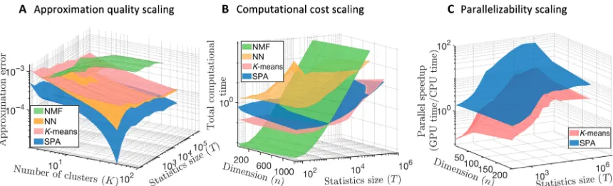
Similar scalability limitations are also the characteristic for the density-based clustering methods [such as the mean shifts (26), the density-based spatial clustering of applications with noise (DBSCAN) (27), and the algorithms based ont-distributed stochastic neighbor embedding (28)], having an iteration complexity in the orders between O(Tlog(T)) (for sparse similarity matrices) andO(T2) (for full similarity matrices). Practical applicability of these methods is restricted to relatively small systems or relies on the ad hoc data reduction steps, i.e.,Tcannot routinely exceed 10,000 or 20,000 when working on commodity hardware (see, e.g., the gray dotted curves with crosses in Fig. 3) (9,28). The cost and quality comparison for the probabilistic approximation methods are shown in Fig. 1. Cost factor becomes decisive when
discre-tizing very large systems, e.g., in biology and geosciences, leading to the necessity of some ad hoc data preprocessing by means of computation-ally cheap methods such asK-means, principal components analysis, and other prereduction steps (29,30).
In the following, we present a method not requiring this ad hoc re-ductional data preprocessing, having the same leading order computa-tional iteration complexityO(nKT) as the cheapK-means algorithm and allowing simultaneously finding discretization that is optimal for models (Eq. 1).
RESULTS
Cost, quality, and parallelizability in scalable probabilistic approximation
Below, we derive the methodology by formulating the discrete approx-imation as an optimization problem. Here, an approxapprox-imation quality of a discretization is expressed as the sum of all distances distS(X(t),GX(t))
between the original statesX(t), and their probabilistic representa-tionsGX(t) obtained for a particular discretizationS= {S1,…,SK}.
For example, minimizing the sum of the squared Euclidean distances distSðXðtÞ;GXðtÞÞ ¼‖XðtÞ ∑Kk¼1GXkðtÞSk‖22with respect toGandS
for a fixed givenXwould allow finding the optimal probabilistic ap-proximations∑Kk¼1GkXðtÞSkof the originaln-dimensional data points
X(t) in the Euclidean space (18–24). Then,Skis ann-dimensional
vector with coordinates of the discrete statek, andGXkðtÞis the
prob-ability thatX(t) belongs to this discrete state (also referred to as a “clusterk,”a“boxk,”or a“reference pointk”in the following).
Moreover, it can be useful to add other minimized quantities to the resulting expression, e.g.,FS(S) (to increase the“quality”of discrete
statesS, to be explained below) andFG(GX) to improve the quality of GX
while simultaneously minimizing the sum of discretization errors. For example, the temporal persistence of the probabilistic representa-tions GX(ift is a time index) can be controlled by FGðGXÞ ¼
1
T∑t‖GXðtþ1Þ GXðtÞ‖(31–33) (measuring the average number of
transitions between discrete states over time), whereasFS(S) can be
chosen as a discrepancy between the actual discretizationSand some a priori available knowledgeSpriorabout it, i.e., asFS(S)=
∣
∣S−Sprior∣|
Fig. 1. Comparing discretization quality (A), full computational cost (B), and algorithm parallelizability (C) for scalable probabilistic approximation (SPA) (blue surfaces) and for common discretization methods:K-means clustering (16,17) (red), NMF (19–24) [in its probabilistic variant called LSD (24), green surfaces], and the discretizing neuronal networks (NNs) based on self-organizing maps (SOMs) (38) (a special form of unsupervised NNs used for discretization, orange surfaces). For every combination of data dimensionnand the data statistics lengthT, methods are applied to 25 equally randomly generated datasets, and the results in each of the curves represent averages over these 25 problems. Parallel speedup in (C) is measured as the ratio of the average timestime(GPU)/time(CPU)needed to reach the same relative tolerance threshold of 10−5on a single GPU [ASUS TURBO-GTX1080TI-11G, with 3584 Compute Unified Device Architecture (CUDA) cores] fortime(GPU)versus a single CPU core (Intel Core i9-7900X CPU) for time(CPU). Further comparisons can be found in the fig. S2. The MATLAB scriptFig1_reproduce.mreproducing these results is available in the repository SPA at https://github. com/SusanneGerber. GPU, graphics processing unit; CPU, central processing unit.
on September 17, 2020
http://advances.sciencemag.org/
(34,35). Consequently, the best possible probabilistic approximation can be defined as a solution of a minimization problem for the followingLwith respect to the variablesSandGX
LðS;GXÞ ¼
∑
Tt¼1distS XðtÞ;GXðtÞþDSFSðSÞ þDGFGðGXÞ ð2Þ
subject to the constraints that enforce that the approximationGXis probabilistic
∑
Kk¼1GXkðtÞ ¼1;andGXkðtÞ≥0 for allkandt ð3Þ
whereDSandDG(both bigger or equal then zero) regulate the relative
importance of the quality criteriaFSandFGwith respect to the
impor-tance of minimizing a sum of discrete approximation errors.
As proven in Theorem 1 in the Supplementary Materials, the minima of problem (Eqs. 2 and 3) can be found by means of an iterative algorithm alternating optimization for variablesGX(with fixedS) and for varia-blesS(with fixedGX). In the following, we provide a summary of the most important properties of this algorithm. A detailed mathemat-ical proof of these properties can be found in Theorems 1 to 3 (as well as in the Lemma 1 to 15 and in the Corollaries 1 to 11) from the Sup-plementary Materials.
In terms of cost, it can be shown that the computational time of the average iteration for the proposed algorithm grows linearly with the sizeTof the available data statistics inX, ifFG(GX) is an additively separable function [meaning that it can be represented asFGðGXÞ ¼
∑T
t¼1φGðGXðtÞÞ]. We refer to the iterative methods for minimization of (Eqs.2 and 3), satisfying this property, as scalable probabilistic approxima-tions (SPAs). Further, if the distance metrics distS(X(t),GX(t)) is either
an Euclidean distance or a Kullback-Leibler divergence, then the over-all iteration cost of SPA grows asO(nKT) (wherenis the system’s orig-inal dimension andKis the number of discrete states). That is, the
computational cost scaling of SPA is the same as the cost scaling of the computationally cheapK-means clustering (16) (see Corollary 6 in the Supplementary Materials for a proof). Moreover, in such a case, it can be shown that the amount of communication between the pro-cessors in the case of the Euclidean distance distS(X(t),GX(t)) during
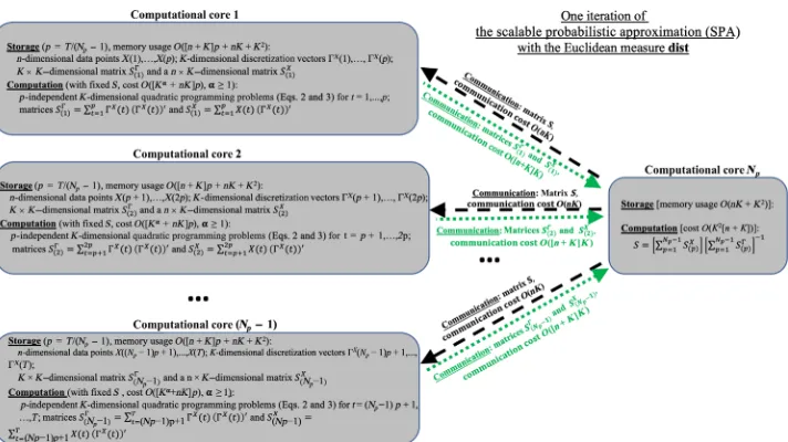
one iteration in a parallel implementation of SPA will be indepen-dent of the sizeTof system’s output and will change proportionally toO(nK) and to the number of the used computational cores. Figure 2 illustrates these properties and shows a principal scheme of the SPA parallelization.
In terms of quality, it is straightforward to validate that several of the common methods are guaranteed to be suboptimal when compared to SPA, meaning that they cannot provide approximations better than SPA on the same system’s dataX. This can be shown rigorously for dif-ferent forms ofK-means (16), e.g., (see Corollary 1 in the Supplemen-tary Materials) and for the different variants of finite element clustering methods on multivariate autoregressive processes with external factors (see Corollary 2 in the Supplementary Materials) (31–33).
Figure 1 shows a comparison of SPA (blue surfaces) to the most common discretization methods for a set of artificial benchmark prob-lems of different dimensionalitynand sizeT(see the Supplementary Materials for a detailed description of the benchmarks). In comparison withK-means, these numerical experiments illustrate that SPA has the same overall cost scaling (Fig. 1B), combined with the substantially bet-ter approximation quality and parallelizability scaling (Fig. 1, A and C).
Computing optimal discretization for Bayesian and Markovian models
Common fitting of Bayesian or Markovian models (Eq. 1) relies on the availability of probabilistic representationsGY(t) andGX(t) and re-quires prior separate discretization ofXandY. There is no guarantee that providing any two of these probabilistic representationsGY(t) and GX
(t) as an input for any of the common computational methods (7–15) forLidentification would result in an optimal model (Eq. 1). That is,
Fig. 2. Parallelization of the SPA algorithm: Communication cost of SPA for every channel is independent of the data sizeTand is linear with respect to the data dimensionn.
on September 17, 2020
http://advances.sciencemag.org/
Bayesian and Markovian models obtained with common methods (7–15) are only optimal for a particular choice of the underlying prob-abilistic representationsGY(t) andGX(t) (which are assumed to be given and fixed for these methods) and are not generally optimal with respect to the change of the discretizationSYandSX.
As proven in Theorem 2 in the Supplementary Materials, the op-timal discretization of the Euclidean variablesXfromRnandYfrom mfor the model (Eq. 1) can be jointly obtained from the family of SPA solutions by minimizing the functionL(Eqs. 2 and 3) for the transformed variableX^D¼ fY;DXgfromRm+n. This variable is built as a concatenation (a merge) of the original variablesYandDX(whereXis multiplied with a tunable scalar parameterD> 0). Scalar parameterD defines the relative weight ofXdiscretization compared toY discret-ization: The largerDis, the more emphasis is placed on minimizing the discretization errors forX. For any combination of parameterDand the discrete dimensionKfrom some predefined range, this SPA opti-mization (Eqs. 2 and 3) is then performed with respect to the tran-sformed variablesSD;K ¼ fSYD;KLD;K;DSXD;Kgand the original variable
GX
D;K (being the discrete probabilistic representation of the original
dataX). Then, the lowern×Kblock of the obtained discretization matrixSD,K(when divided withD) provides an optimal discretization
matrixSXforX.
In the case of Bayesian models, prediction of valuesYpred(s) from the data vectorX(s) (which was not a part of the original datasetX) is ap-proached in two steps: (step 1) computing the discretizationGX(s) by solving theK-dimensional quadratic optimization problem GX
(s) = argminG||X(s)−SXGX(s)||22, such that theKelements ofGX(s)
sum up to one and are all non-negative (conditions for existence, uniqueness, and stability of this problem solution are investigated in Lemma 9, 11, 12, 14, and 17 in the Supplementary Materials); and (step 2) multiplying the obtained discretization vectorGX(s) with the upperm×Kblock of the SPA matrixSD,Kprovides a prediction
Ypred(s), i.e.,YpredðsÞ ¼SY
D;KLD;KGXðsÞ. Note that this two-step
pre-diction procedure would not require the explicit estimation ofLD,K
andSY
D;K.Y pred
(s) is computed by a direct multiplication of the vector GX
(s) (from the step 1) with the upperm×Kblock of the SPA matrix SD,K. This is the procedure deployed in the computational analysis of
benchmarks described below. If required, then discretization matrix
SY
D;K and the stochastic matrixLD,Kcan be disentangled from the
upperm×Kblock ofSD,Kby means of the standard matrix
factori-zation algorithms (18–24).
In case of Markovian models, whenY(s) is defined asX(s + 1), K×Ktransition matrixLD,Kobtained from such a matrix
factori-zation also allows the computation of theN-step predictions ofGX, as GX
(s + N) =LN
D;KG X
(s) from the discrete approximationGX(s) of the data pointX(s) (from step 1). Then, in step 2, theN-step prediction Ypred(s+N) is obtained asYpredðsþNÞ ¼SY
D;KLND;KGXðsÞ.
Alternative-ly, to enforce thatY(s) is strictly defined asX(s + 1) in the case of the Markov processes and that the two discretization operatorsSY
D;K and
SX
D;K should be the same and provide a discretization of the same
Eu-clidean datasetX, one can impose an additional equality constraint
SY
D;K ¼SXD;Kto the SPA optimization problem (Eqs. 2 and 3) and split
theS-optimization step of the iterative SPA algorithm into two substeps: (substep 1) the minimization of (Eqs. 2 and 3) with respect toSX
D;Kfor fixed
values ofLD,KandGXand (substep 2) the minimization of (Eqs. 2 and 3)
with respect toLD,Kfor fixed values ofSXD;K andG X
. This procedure results in a monotonic minimization of the SPA problem (Eqs. 2 and 3) and provides direct estimates of theK×KMarkovian transition matrixLD,Kand then×Kdiscretization matrixSXD;Kin the Markovian
case. Note that this procedure does not provide an explicit Markov model that directly relatesX(s + N) toX(s). The two-step procedure described above results in an implicit Markovian modelGX(s + N) = LN
D;KG X
(s), operating on the level ofK-dimensional discrete probability densitiesGX. The optimal combination of tunable parametersDandK for the optimal discretization in model (Eq. 1) is obtained by applying standard model selection criteria (36) (e.g., using information criteria or approaches such as multiple cross-validations).
These procedures of simultaneous discretization and model infer-ence rely on the assumption that bothXandYare Euclidean data. If this is not the case, then the data have to be transformed to Euclidean before applying the SPA. In the case of time series with equidistant time steps, Euclidean transformation (or Euclidean embedding) is achieved by the so-called Takens embedding transformation, when instead of analyzing single realizations of the dataX(s) inRn, one considers transformed data points given as a whole time sequence [X(s),X(s− 1),…,X(s−dim)] inRn(dim+1). The justification of this procedure is
provided by the Takens theorem (37), proving that this transformation embeds any sufficiently smooth non-Euclidean attractive manifold of a dynamic system into Euclidean space. This procedure is deployed for the time series data analysis benchmarks considered below, an analytical example of such an embedding transformation for autoregressive models is provided in Corollary 2 in the Supplementary Materials. Al-ternatively, in the case of the classification problems for the data that are not time series, one can apply SPA framework (Eqs. 2 and 3) to the transformed dataXtrans(s)= F(X(s),w),s= 1,…,T.Fis a nonlinear Eu-clidean transformation performed, e.g., by a neuronal network (NN) that relies on a tunable parameter vectorw(a vector of network weights and biases). Then, the iterative minimization of (Eqs. 2 and 3) can be augmented straightforwardly with an optimization with respect to an additional parameter vectorwof this NN transformation. Below, this kernelized SPA procedure will be referred to as SPA + NN and used for the analysis of classification benchmarks from Fig. 3.
Sensitivity analysis and feature selection with SPA
After the discretization problem is solved, an optimal discrete repre-sentationGX(t) can be computed for any continuous pointX(t). Ob-tained vectorGX(t)containsKprobabilitiesGkXðtÞ for a pointX(t) to belong to each particular discrete stateSkand allows computing the
reconstructionXrec(t) of the pointX(t) asXrec(t) =SGX(t). In this sense, procedure (Eqs. 2 and 3) can be understood as the process of finding an optimal discrete probabilistic data compression, such that the aver-age data reconstruction error [measured as a distance betweenX(t) and Xrec(t)] is minimized.
In the following, we refer to the particular dimensions ofXas features and consider a problem of identifying sets of features that are most relevant for the discretization. The importance of any feature/ dimensionjofXfor the fixed discrete statesScan be measured as an average sensitivity of the obtained continuous data reconstructions Xrec(t) with respect to variations of the original dataX(t) along this
dimensionj. For example, it can be measured by means of the average derivative normIðjÞ ¼1
T∑t‖∂XrecðtÞ=∂XjðtÞ‖22. For every dimensionj
ofX(t), this quantityI(j) probes an average impact of changes in the dimension jof X(t) on the resulting data reconstructionsXrec(t). Dimensionsjthat have the highest impact on discretization will have the highest values ofI(j), whereas the dimensionsjthat are irrelevant for the assignation to discrete states will haveI(j) close to 0.
At first glance, direct computation of the sensitivitiesI(j) could seem too expensive for realistic applications with large data statistics sizeT
on September 17, 2020
http://advances.sciencemag.org/
and in high problem dimensions and due to the a priori unknown smoothness of the derivate∂∂XXrecjððttÞÞin the multidimensional space of features. However, as proven in Theorem 3 in the Supplementary Materials, in the case of discretizations obtained by solving the problem (Eqs. 2 and 3) for the Euclidean distance measure dist, respective deriva-tives∂∂XXrecjððttÞÞare always piecewise constant functions ofXj(t) if the
sta-tistics sizeTis sufficiently large. This nice property of derivatives allows a straightforward numerical computation ofI(j) forK> 2 and an exact analytical computation ofIforK= 2. It turns out that forK= 2, the importance of every original data dimensionjcan be directly measured asðS2;jS1;jÞ2=‖S2S1‖22. That is, discretization sensitivityI(j) for the
featurejis proportional to the squared difference between the discret-ization coordinatesS1,jandS2,jin this dimensionj. The smaller the
difference between the coordinates in this dimension, the lower is the impact of this particular featurejon the overall discretization.
It is straightforward to verify (see Corollary 9 and Theorem 3 in the Supplementary Materials for a proof) that the feature sensitivity functionI¼∑jIðjÞ has a quadratic upper boundI≤ ∑j,k1,k2(Sk1(j)−
Sk2(j))
2. SettingF
S(S) in Eq. 2 asFS(S) =∑j,k1,k2(Sk1(j)−Sk2(j))
2for
any given combination of integerKand scalarDS≥0, minimizing
(Eqs. 2 and 3) would then result in a joint simultaneous and scalable solution of the optimal discretization and feature selection problems. Overall, the numerical iteration cost of this procedure will be againO (nKT). ChangingDScontrols the number of features: The largerDSis,
the fewer features (i.e., particular dimensions of the original data vector X) remain relevant in the obtained discretization. The optimal value of DScan again be determined by means of standard model validation
criteria (36). In the SPA results from Figs. 3 and 4 (blue curves), we use this form ofFS(S), setDG= 0, and deploy the multiple cross-validation,
a standard model selection approach from machine learning, to determine the optimalDSand an optimal subset of relevant features for any given
numberKof discrete states (clusters).
Applications to classification and prediction problems from natural sciences
Next, we compare the discretization performance of SPA to the ap-proximation errors of the common methods, includingK-means (16), soft clustering methods based on Bayesian mixture models (17) (such as GMMs), density-based clustering (DBSCAN) (27), and NN discretization methods (self-organizing maps, SOMs) (38). To compare the performances of these methods, we use ob-tained discretization in parametrization of the Bayesian/Markovian models (Eq. 1), as well as in parametrization of NNs (38), on several classification and time series analysis problems from different areas.
To prevent overfitting, we deploy the same multiple cross-validation protocol (36,39) adopted in machine learning for all tested methods. Here, the data are randomly subdivided into the training set (75% of the data), where the discretization and classification/predic-tion models are trained and performance quality measures (ap-proximation, classification, and prediction errors) are then determined on the remaining 25% of validation data (not used in the training). For each of the methods, this procedure of random data subdivision, training, and validation is repeated 100 times; Figs. 3 and 4 provide the resulting average performance curves for each of the tested methods. In both classification and time series predic-tion applicapredic-tions of SPA, no persistence in thet-ordering was assumed a priori by settingDGin (Eq. 2) to 0. This means not imposing any a priori persistent ordering in tfor the probabilistic representations {GX(1),…, {GX(T)} and justifying an application of the common multiple cross-validation procedure (36) (which implies random reshufflings intand subdivisions of data into training and validation sets) for a selection of optimal values forKandDS. MATLAB scripts reproducing
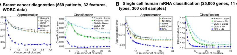
the results are available in the repository SPA at https://github.com/ SusanneGerber. Figure 3 shows a comparison of approximation and classification performances for two problems of labeled data analysis from biomedicine and bioinformatics: (Fig. 3A) for a problem of breast cancer diagnostics based on x-ray image analysis (40) and (Fig. 3B) for a problem of single-cell human mRNA classification (41). In these pro-blems, variableX(t) is a continuous (and real valued) set of collected features that have to be brought in relation to the discrete set of labels Y(t). In case of the breast cancer diagnostics example (40), (Fig. 3A) indextdenotes patients and goes from 1 to 569,X(t) contains 32 image features, andY(t) can take two values“benign”or“malignant.”In the case of the single-cell human mRNA classification problem (41), (Fig. 3B) indextgoes from 1 to 300 (there are 300 single-cell probes),X(t) contains expression levels for 25,000 genes, andY(t) is a label denoting one of the 11 cell types (e.g.,“blood cell,” “glia cell,”etc.). In both cases, the ordering of data instancestin the datasets is arbitrary and is as-sumed not to contain any a priori relevant information related to time (such as temporal persistence of the ordering along the indext).
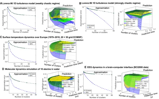
Figure 4 summarizes results for five benchmark problems from time series analysis and prediction: for the Lorenz-96 benchmark system (42) modeling turbulent behavior in one dimension, in a weakly chaotic (Fig. 4A) and in the strongly chaotic (Fig. 4B) regimes; (Fig. 4C) for 45 years (T= 16,433 days) of historical Eu-ropean Centre for Medium-Range Weather Forecasts (ECMWF)– resimulated 2-m height daily air temperature anomalies (deviations from the mean seasonal cycle) time series on a 18 by 30 grid over Fig. 3. Classification problems: Comparing approximation and classification performances of SPA (blue curves) to the common methods on biomedical applications (40,41).Common methods includeK-means clustering (dotted lines), SOM (brown), pattern recognition NNs (dashed lines), GMMs (cyan), density-based clustering (gray dotted lines with crosses), and Bayesian models (Eq. 1) (Bayes; dotted lines). Approximation error is measured as the multiply cross-validated average squared Euclidean norm of difference between the true and the discretized representations for validation data. Classification error is measured as the multiply cross-validated average total variation norm between the true and the predicted classifications for validation data. WDBC, Wisconsin Diagnostic Breast Cancer database.
on September 17, 2020
http://advances.sciencemag.org/
the continental Europe and a part of the Northern Atlantic (43), pro-vided by the ECMWF; (Fig. 4D) for the biomolecular dynamics of a 10–alanine peptide molecule in water (15); and (Fig. 4E) for the electrical activity of the brain measured in various brain-computer interaction (BCI) regimes obtained with the 64-channel electroencephalography and provided for open access by the BCI2000 consortium (44).
As can be seen from the Figs. 3 and 4, SPA tends to reach its approx-imation quality plateau earlier (i.e., with much smallerK) but is gener-ally much more accurate, with a discretization performance improvement factor ranging from two to four (for breast cancer diag-nostics example, for single-cell mRNA classification, for the tempera-ture data over Europe, and for the molecular dynamics application). For the Lorenz-96 turbulence applications (42) and for the brain activity application (44), discretization obtained by SPA is 10 to 100 times better than the discretization from common methods, being at the same level of computational cost as the popularK-means clustering (16).
When evaluating a prediction performance of different models for a particular system, it is important to compare it with the trivial pre-diction strategies called mean value prepre-diction and persistent predic-tion. The mean value prediction strategy predicts the next state of the system to be an expectation value over the previous already observed states and is an optimal prediction strategy for stationary independent and identically distributed processes such as the Gaussian process. The persistent prediction strategy is predicting the next state of the system to be the same as its current state. This strategy is particularly
success-ful and is difficult to be beaten for the systems with more smooth ob-servational time series, e.g., for the intraday surface temperature dynamics. As it can be seen from the fig. S3, among all other considered methods (K-means, NNs, SOM, and mixture models), on-ly the SPA discretization combined with the Markov models (Eq. 1) allow outperforming both the mean value and the persistent predic-tions for all of the considered systems.
DISCUSSION
Computational costs become a limiting factor when dealing with big systems. The exponential growth in the hardware performance ob-served over the past 60 years (the Moore’s law) is expected to end in the early 2020s (45). More advanced machine learning approaches (e.g., NNs) exhibit the cost scaling that grows polynomial with the dimension and the size of the statistics, rendering some form of ad hoc preprocessing and prereduction with more simple approaches (e.g., clustering methods) unavoidable for big data situations. However, these ad hoc preprocessing steps might impose a strong bias that is not easy to quantify. At the same time, lower cost of the method typically goes hand-in-hand with the lower quality of the obtained data represen-tations (see Fig. 1). Since the amounts of collected data in most of the natural sciences are expected to continue their exponential growth in the near future, pressure on computational performance (quality) and scaling (cost) of algorithms will increase.
Fig. 4. Prediction problems in time series analysis: Comparing approximation and prediction performances of SPA (blue curves) to the common methods on open-source datasets (15,42–44).Common methods includeK-means clustering (K-means; dark green) in combinations with pattern recognition recurrent NNs (yellow and light green) and Markov models (Eq. 1) (dark green). Approximation and the prediction errors are measured in the average squared Euclidean norm of deviations between the true and the predicted system states for the validation data (i.e., for data not used in the model fitting). EEG, electroencephalogram.
on September 17, 2020
http://advances.sciencemag.org/
Instead of solving discretization, feature selection, and predic-tion problems separately, the introduced computapredic-tional procedure (SPA) solves them simultaneously. The iteration complexity of SPA scales linearly with data size. The amount of communication be-tween processors in the parallel implementation is independent of the data size and linear with the data dimension (Fig. 2), making it appropriate for big data applications. Hence, SPA did not require any form of data prereduction for any of the considered applica-tions. As shown in the Fig. 1, having essentially the same iteration cost scaling as the very popular and computationally very cheapK -means algorithm (16,17), SPA allows achieving substantially higher approximation quality and a much higher parallel speedup with the growing sizeTof the data.
Applications to large benchmark systems from natural sciences (Figs. 3 and 4) reveal that these features of SPA allow a marked improve-ment of approximation and cross-validated data-driven prediction qua-lities, combined with a massive reduction of computational cost. For example, computing the next-day surface temperature anomalies for Europe (e.g., at the ECMWF) currently relies on solving equations of atmosphere motion numerically performed on supercomputers (43). Discretization and cross-validated data-driven prediction results for the same online resimulated daily temperature data provided in the Fig. 4C were obtained on a standard Mac PC, exhibiting a mean error of 0.75°C for the 1-day ahead surface air temperature anomalies com-putations (approximately 40% smaller than the current next-day pre-diction errors by weather services).
These probability-preserving and stable predictionsGY(t) can be accomplished very cheaply with the Bayesian or Markovian model (Eq. 1) from the available SPA discretization (Eqs. 2 and 3), just by comput-ing the product of the obtainedK×KBayesian matrixLwith the K× 1 discretization vectorGX(t). OptimalKwas in the orders of 10 to 40 for all of the considered applications from Figs. 3 and 4. The iteration cost of this entire data-driven computation scales linearly, re-sulting in orders of magnitude speedup as compared to the predictions based on the entire system’s simulations. These results indicate a potential to use efficient and cheap Bayesian and Markovian descriptive models for a robust automated classification and data-driven cross-validated predictive computations in many realistic systems across natural sciences. However, an assumption about thetindependence of the conditional probability matrixLin (Eq. 1), which allowed apply-ing common model selection procedures from machine learnapply-ing, can limit the applicability of the method in the nonstationary situations, whenLin (Eq. 1) becomestdependent. Addressing the nonstationarity problem will become an important issue for future applications to these systems.
MATERIALS AND METHODS
We used the standard MATLAB functionskmeans(),fitgmdist(),
patternnet(), andsom()to compute the results of the common methods
(K-means, GMM, NN, and SOM) in Figs. 1, 3, and 4. To avoid being trapped in the local optima and to enable a unified comparison of all methods, we used 10 random initializations and selected the results with the best approximation quality measure for the training sets. In case of the pattern recognition NNs (evaluated in the classification and predic-tion performance subfigures of Figs. 3 and 4) in each of the instances of the multiple cross-validation procedure, we repeated the network fitting for the numbers of neurons in the hidden layer ranging between 1 and 15 and selected the results with the best classification/prediction
perform-ances for the training set. We implemented the LSD algorithm from Fig. 1 in MATLAB according to the literature description (24) and provided it for open access. SPA algorithms developed and used during the cur-rent study are also available in open access as MATLAB code at https:// github.com/SusanneGerber.
SUPPLEMENTARY MATERIALS
Supplementary material for this article is available at http://advances.sciencemag.org/cgi/ content/full/6/5/eaaw0961/DC1
Description of the synthetic data problems (used in the Fig. 2 of the main manuscript) General SPA formulation
SPA in the Euclidean space Optimality conditions The solution ofSsubproblem The solution ofGsubproblem
Computing optimal discretizations for Bayesian and Markovian models Sensitivity and feature selection with SPA in the Euclidean space Appendix
Fig. S1. Distributed solution ofGproblem. Fig. S2. Comparison of different measures. Fig. S3. Comparison of one time-step predictions.
REFERENCES AND NOTES
1. A. Stuart, A. Humphries, Dynamical systems and numerical analysis, inCambridge Monographs on Applied Mathematics(Cambridge Univ. Press, 1998), vol. 8.
2. A. J. Chorin, O. H. Hald,Stochastic Tools in Mathematics and Science(Springer, ed. 3, 2013). 3. D. B. Rubin, Bayesian inference for causal effects: The role of randomization.Ann. Stat.6,
34–58 (1978).
4. D. B. Rubin,Bayesian Data Analysis(Chapman and Hall/CRC Texts in Statistical Science, ed. 3, 2013).
5. Ch. Schütte, M. Sarich, Metastability and Markov state models in molecular dynamics: Modeling, analysis, algorithmic approaches, inCourant Lecture Notes in Mathematics
(American Mathematical Soc., 2013), vol. 24.
6. A. N. Langville, C. D. Meyer,Google’s PageRank and Beyond: The Science of Search Engine Rankings(Princeton Univ. Press, 2006).
7. C. Schütte, W. Huisinga, P. Deuflhard, Transfer operator approach to conformational dynamics in biomolecular systems, inErgodic Theory, Analysis, and Efficient Simulation of Dynamical Systems, B. Fiedler, Ed. (Elsevier, 2001), pp. 191–223.
8. P. Deuflhard, M. Weber, Robust Perron cluster analysis in conformation dynamics.
Lin. Algebra Appl.398, 161–184 (2005).
9. S. Gerber, S. Olsson, F. Noé, I. Horenko, A scalable approach to the computation of invariant measures for high-dimensional Markovian systems.Sci. Rep.8, 1796 (2018).
10. G. Froyland, K. Padberg, Almost-invariant sets and invariant manifolds: Connecting probabilistic and geometric descriptions of coherent structures in flows.Physica D Nonlin. Phenom.238, 1507–1523 (2009).
11. A. Majda, R. Abramov, M. Grote,Information Theory and Stochastics for Multiscale Nonlinear Systems(CRM monograph series, American Mathematical Soc., 2005). 12. M. Weber, S. Kube, Robust Perron cluster analysis for various applications in
computational life science.Lect. Notes Comp. Sci.3695, 55–66 (2005).
13. T. Hofmann, Probabilistic latent semantic analysis, inProceedings of the 15th Annual Conference on Uncertainty in Artificial Intelligence (UAI’99)(Morgan Kaufmann Publishers, 1999), pp. 289–296.
14. S. Gerber, I. Horenko, Toward a direct and scalable identification of reduced models for categorical processes.Proc. Natl. Acad. Sci. U.S.A.114, 4863–4868 (2017).
15. S. Gerber, I. Horenko, On inference of causality for discrete state models in a multiscale context.Proc. Natl. Acad. Sci. U.S.A.111, 14651–14656 (2014).
16. J. A. Hartigan, M. A. Wong, Algorithm AS 136: A K-means clustering algorithm.
J. R. Stat. Soc. C1, 100–108 (1979).
17. P. D. McNicholas,Mixture Model-Based Classification(CRC Press, ed. 1, 2016). 18. P. Paatero, U. Tapper, Positive matrix factorization: A non-negative factor model with
optimal utilization of error estimates of data values.Environmetrics5, 111–126 (1994). 19. D. D. Lee, H. S. Seung, Learning the parts of objects by nonnegative matrix factorization.
Nature401, 788–791 (1999).
20. D. L. Donoho, V. Stodden, Learning the parts of objects by nonnegative matrix factorization. When does non-negative matrix factorization give a correct decomposition into parts? inAdvances in Neural Information Processing Systems, S. Thrun, L. Saul, B. Schölkopf, Eds. (MIT Press, 2004), vol. 24.
on September 17, 2020
http://advances.sciencemag.org/
21. C. H. Q. Ding, T. Li, M. I. Jordan, Convex and semi-nonnegative matrix factorizations.
IEEE Trans. Pattern Anal. Mach. Intell.32, 45–55 (2010).
22. C.-J. Lin, Projected gradient methods for nonnegative matrix factorization.
Neural Comput.19, 2756–2779 (2007).
23. C. Ding, T. Li, W. Peng, Nonnegative matrix factorization and probabilistic latent semantic indexing: Equivalence, chi-square statistic, and a hybrid method, inProceedings of the 21st National Conference on Artificial Intelligence and the 18th Innovative Applications of Artificial Intelligence Conference(AAAI Press, 2006), vol. 1, pp. 342–347.
24. R. Arora, M. R. Gupta, A. Kapila, M. Fazel, Similarity-based clustering by left-stochastic matrix factorization.J. Mach. Learn. Res.14, 1417–1452 (2013).
25. A. Ng, M. Jordan, Y. Weiss, On spectral clustering: Analysis and an algorithm, inAdvances in Neural Information Processing Systems (NIPS)(MIT Press, 2002), vol. 14, pp. 849–856. 26. Y. Cheng, Mean shift, mode seeking and clustering.IEEE Trans. Pattern Anal. Mach. Intell.
17, 790–799 (1995).
27. M. Ester, H.-P. Kriegel, J. Sander, X. Xu, A density-based algorithm for discovering clusters in large spatial databases with noise, inProceedings of the Second International Conference on Knowledge Discovery and Data Mining (KDD’96)(AAAI Press, 1996), pp. 226–231. 28. L. van der Maaten, Accelerating t-SNE using tree-based algorithms.J. Mach. Learn. Res.
15, 3221–3245 (2014).
29. P. D’haeseleer, How does gene expression clustering work?Nat. Biotechnol.23, 1499–1501 (2005).
30. C. Cassou, Intraseasonal interaction between the Madden–Julian Oscillation and the North Atlantic Oscillation.Nature455, 523–527 (2008).
31. P. Metzner, L. Putzig, I. Horenko, Analysis of persistent nonstationary time series and applications.Commun. Appl. Math. Comput. Sci.7, 175–229 (2012).
32. T. J. O’Kane, R. J. Matear, M. A. Chamberlain, J. S. Risbey, B. M. Sloyan, I. Horenko, Decadal variability in an OGCM Southern Ocean: Intrinsic modes, forced modes and metastable states.Ocean Model.69, 1–21 (2013).
33. N. Vercauteren, R. Klein, A clustering method to characterize intermittent bursts of turbulence and interaction with submesomotions in the stable boundary layer.
J. Atmos. Sci.72, 1504–1517 (2015).
34. R. Tibshirani, Regression shrinkage and selection via the lasso.J. R. Stat. Soc. B58, 267–288 (1996).
35. S. Gerber, I. Horenko, Improving clustering by imposing network information.Sci. Adv.1, e1500163 (2015).
36. K. Burnham, D. Anderson,Model Selection and Multimodel Inference: A Practical Information-Theoretic Approach(Springer, ed. 2, 2002).
37. F. Takens, Detecting strange attractors in turbulence, inDynamical Systems and Turbulence, Lecture Notes in Mathematics, D. A. Rand, L.-S. Young, Eds. (Springer-Verlag, 1981), vol. 898, pp. 366–381.
38. T. Kohhonen,Self-Organising Maps(Springer Series in Information Sciences, ed. 3, 2001), vol. 30.
39. L. Trippa, L. Waldron, C. Huttenhower, G. Parmigiani, Bayesian nonparametric cross-study validation of prediction methods.Ann. Appl. Stat.9, 402–428 (2015).
40. W. H. Wolberg, W. N. Street, O. L. Mangasarian, Machine learning techniques to diagnose breast cancer from image-processed nuclear features of fine needle aspirates.
Cancer Lett.77, 163–171 (1994).
41. A. A. Pollen, T. J. Nowakowski, J. Shuga, X. Wang, A. A. Leyrat, J. H. Lui, N. Li, L. Szpankowski, B. Fowler, P. Chen, N. Ramalingam, G. Sun, M. Thu, M. Norris, R. Lebofsky, D. Toppani, D. W. Kemp II, M. Wong, B. Clerkson, B. N. Jones, S. Wu, L. Knutsson, B. Alvarado, J. Wang, L. S. Weaver, A. P. May, R. C. Jones, M. A. Unger, A. R. Kriegstein, J. A. A. West, Low-coverage single-cell mRNA sequencing reveals cellular heterogeneity and activated signaling pathways in developing cerebral cortex.Nat. Biotechnol.32, 1053–1058 (2014).
42. E. Lorenz, Predictability: A problem partly solved, inProceedings of the ECMWF Seminar on Predictability(ECMWF, 1996), vol. 1, pp. 1–18.
43. D. P. Dee, S. M. Uppala, A. J. Simmons, P. Berrisford, P. Poli, S. Kobayashi, U. Andrae, M. A. Balmaseda, G. Balsamo, P. Bauer, P. Bechtold, A. C. M. Beljaars, L. van de Berg, J. Bidlot, N. Bormann, C. Delsol, R. Dragani, M. Fuentes, A. J. Geer, L. Haimberger, S. B. Healy, H. Hersbach, E. V. Hólm, L. Isaksen, P. Kållberg, M. Köhler, M. Matricardi, A. P. McNally, B. M. Monge-Sanz, J.-J. Morcrette, B.-K. Park, C. Peubey, P. de Rosnay, C. Tavolato, J.-N. Thépaut, F. Vitart, The ERA-Interim reanalysis: Configuration and performance of the data assimilation system.Q. J. R. Meteorol. Soc.137, 553–597 (2011).
44. G. Schalk, J. Mellinger,A Practical Guide to Brain–Computer Interfacing with BCI2000
(Springer, ed. 1, 2010).
45. H. N. Khan, D. A. Hounshell, E. R. H. Fuchs, Science and research policy at the end of Moore’s law.Nat. Electron.1, 14–21 (2018).
Acknowledgments:We thank G. Ciccotti (La Sapienza, Rome), M. Weiser (ZIB, Berlin), D. L. Donoho (Standford University), M. Wand (JGU, Mainz), P. Gagliardinin (USI, Lugano), R. Klein (FU, Berlin), and F. Bouchet (ENS, Lyon) for helpful comments about the manuscript. Funding:We acknowledge the financial support from the German Research Foundation DFG (“Mercator Fellowship”of I.H. in the CRC 1114“Scaling cascades in complex systems”). S.G. acknowledges the financial support from the DFG (in the CRC 1193“Neurobiology of resilience to stress-related mental dysfunction: From understanding mechanisms to promoting preventions”). The work of M.N. was supported by the Research Center For Emergent Algorithmic Intelligence at the University of Mainz funded by the Carl-Zeiss Foundation.Author contributions:S.G. and I.H. designed the research, wrote the main manuscript, and produced results in Figs. 3 and 4. L.P. and I.H. produced results in Fig. 1 and proved Theorems 1 to 3 and Lemmas in the Supplementary Materials. M.N. prepared the data and participated in the analysis of single-cell mRNA data (Fig. 3B).Competing interests:The authors declare that they have no competing interests.Data and materials availability:All data needed to evaluate the conclusions in the paper are present in the paper and/or the Supplementary Materials. Additional data related to this paper may be requested from the authors.
Submitted 16 November 2018 Accepted 22 November 2019 Published 29 January 2020 10.1126/sciadv.aaw0961
Citation:S. Gerber, L. Pospisil, M. Navandar, I. Horenko, Low-cost scalable discretization, prediction, and feature selection for complex systems.Sci. Adv.6, eaaw0961 (2020).
on September 17, 2020
http://advances.sciencemag.org/
S. Gerber, L. Pospisil, M. Navandar and I. Horenko
DOI: 10.1126/sciadv.aaw0961 (5), eaaw0961.
6
Sci Adv
ARTICLE TOOLS http://advances.sciencemag.org/content/6/5/eaaw0961
MATERIALS
SUPPLEMENTARY http://advances.sciencemag.org/content/suppl/2020/01/27/6.5.eaaw0961.DC1
REFERENCES
http://advances.sciencemag.org/content/6/5/eaaw0961#BIBL This article cites 27 articles, 3 of which you can access for free
PERMISSIONS http://www.sciencemag.org/help/reprints-and-permissions
Terms of Service Use of this article is subject to the
is a registered trademark of AAAS.
Science Advances
York Avenue NW, Washington, DC 20005. The title
(ISSN 2375-2548) is published by the American Association for the Advancement of Science, 1200 New
Science Advances
License 4.0 (CC BY-NC).
Science. No claim to original U.S. Government Works. Distributed under a Creative Commons Attribution NonCommercial Copyright © 2020 The Authors, some rights reserved; exclusive licensee American Association for the Advancement of
on September 17, 2020
http://advances.sciencemag.org/