Dynamic Conditional Random Fields: Factorized Probabilistic Models for Labeling and Segmenting Sequence Data

Dynamic Conditional Random Fields: Factorized Probabilistic Models

for Labeling and Segmenting Sequence Data

Charles Sutton [email protected]

Andrew McCallum [email protected]

Khashayar Rohanimanesh∗ [email protected]

Department of Computer Science University of Massachusetts 140 Governors Drive

Amherst, Massachusetts 01003, USA

Editor: Michael Collins

Abstract

In sequence modeling, we often wish to represent complex interaction between labels, such as when performing multiple, cascaded labeling tasks on the same sequence, or when long-range dependen-cies exist. We present dynamic conditional random fields (DCRFs), a generalization of linear-chain conditional random fields (CRFs) in which each time slice contains a set of state variables and edges—a distributed state representation as in dynamic Bayesian networks (DBNs)—and param-eters are tied across slices. Since exact inference can be intractable in such models, we perform approximate inference using several schedules for belief propagation, including tree-based repa-rameterization (TRP). On a natural-language chunking task, we show that a DCRF performs better than a series of linear-chain CRFs, achieving comparable performance using only half the training data. In addition to maximum conditional likelihood, we present two alternative approaches for training DCRFs: marginal likelihood training, for when we are primarily interested in predicting only a subset of the variables, and cascaded training, for when we have a distinct data set for each state variable, as in transfer learning. We evaluate marginal training and cascaded training on both synthetic data and real-world text data, finding that marginal training can improve accuracy when uncertainty exists over the latent variables, and that for transfer learning, a DCRF trained in a cascaded fashion performs better than a linear-chain CRF that predicts the final task directly. Keywords: conditional random fields, graphical models, sequence labeling

1. Introduction

The problem of labeling and segmenting sequences of observations arises in many different areas, including bioinformatics, music modeling, computational linguistics, speech recognition, and in-formation extraction. Dynamic Bayesian Networks (DBNs) (Dean and Kanazawa, 1989; Murphy, 2002) are a popular method for probabilistic sequence modeling, because they exploit structure in the problem to compactly represent distributions over multiple state variables. Hidden Markov Models (HMMs), an important special case of DBNs, are a classical method for speech recognition (Rabiner, 1989) and part-of-speech tagging (Manning and Sch ¨utze, 1999). More complex DBNs have been used for applications as diverse as robot navigation (Theocharous et al., 2001), audio-visual speech recognition (Nefian et al., 2002), activity recognition (Bui et al., 2002), information

extraction (Skounakis et al., 2003; Peshkin and Pfeffer, 2003), and automatic speech recognition (Bilmes, 2003).

DBNs are typically trained to maximize the joint probability distribution p(y,x) of a set of observation sequences x and labels y. However, when the task does not require the ability to generate x, such as in segmenting and labeling, modeling the joint distribution is a waste of modeling effort. Furthermore, generative models often must make problematic independence assumptions among the observed nodes in order to achieve tractability. In modeling natural language, for example, we may wish to use features of a word such as its identity, capitalization, prefixes and suffixes, neighboring words, membership in domain-specific lexicons, and category in semantic databases like WordNet—features which have complex interdependencies. Generative models that represent these interdependencies are in general intractable; but omitting such features or modeling them as independent has been shown to hurt accuracy (McCallum et al., 2000).

A solution to this problem is to model instead the conditional probability distribution p(y|x). The random vector x can include arbitrary, non-independent, domain-specific feature variables. Be-cause the model is conditional, the dependencies among the features in x do not need to be explicitly represented. Conditionally-trained models have been shown to perform better than generatively-trained models on many tasks, including document classification (Taskar et al., 2002), part-of-speech tagging (Ratnaparkhi, 1996), extraction of data from tables (Pinto et al., 2003), segmentation of FAQ lists (McCallum et al., 2000), and noun-phrase segmentation (Sha and Pereira, 2003).

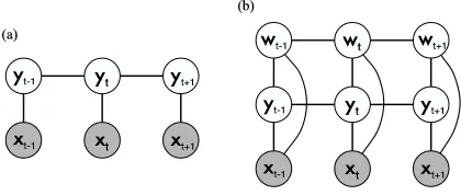
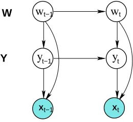
Conditional random fields (CRFs) (Lafferty et al., 2001; Sutton and McCallum, 2006) are undi-rected graphical models of the conditional distribution p(y|x). Early work on CRFs focused on the linear-chain structure (depicted in Figure 1) in which a first-order Markov assumption is made among labels. This model structure is analogous to conditionally-trained HMMs, and has efficient exact inference algorithms. Often, however, we wish to represent more complex interaction between labels—for example, when longer-range dependencies exist between labels, when the state can be naturally represented as a vector of variables, or when performing multiple cascaded labeling tasks on the same input sequence.

In this paper, we introduce dynamic CRFs (DCRFs), which are a generalization of linear-chain CRFs that repeat structure and parameters over a sequence of state vectors. This allows us to both represent distributed hidden state and complex interaction among labels, as in DBNs, and to use rich, overlapping feature sets, as in conditional models. For example, the factorial structure in Figure 1(b), which we call a factorial CRF (FCRF), includes links between cotemporal labels, ex-plicitly modeling limited probabilistic dependencies between two different label sequences. Other types of DCRFs can model higher-order Markov dependence between labels (Figure 2), or incorpo-rate a fixed-size memory. For example, a DCRF for part-of-speech tagging could include for each word a hidden state that is true if any previous word has been tagged as a verb.

Any DCRF with multiple state variables can be collapsed into a linear-chain CRF whose state space is the cross-product of the outcomes of the original state variables. However, such a linear-chain CRF needs exponentially many parameters in the number of variables. Like DBNs, DCRFs represent the joint distribution with fewer parameters by exploiting conditional independence rela-tions.

always cascade through the chain, causing errors in the final output. This problem can be solved by jointly representing the subtasks in a single graphical model, both explicitly representing their dependence, and preserving uncertainty between them. DCRFs can represent dependence between subtasks solved using finite-state transducers, such as phonological and morphological analysis, POS tagging, shallow parsing, and information extraction.

More specifically, in information extraction and data mining, McCallum and Jensen (2003) argue that the same kind of probabilistic unification can potentially be useful, because in many cases, we wish to mine a database that has been extracted from raw text. A unified probabilistic model for extraction and mining can allow data mining to take into account the uncertainty in the extraction, and allow extraction to benefit from emerging patterns produced by data mining. The applications here, in which DCRFs are used to jointly perform multiple sequence labeling tasks, can be viewed as an initial step toward that goal.

In this paper, we evaluate DCRFs on several natural-language processing tasks. First, a factorial CRF that learns to jointly predict parts of speech and segment noun phrases performs better than cascaded models that perform the two tasks in sequence. Also, we compare several schedules for belief propagation, showing that although exact inference is feasible, on this task approximate inference has lower total training time with no loss in testing accuracy.

In addition to conditional maximum likelihood training, we present two alternative training methods for DCRFs: marginal training and cascaded training. First, in some situations, we are primarily interested in predicting a few output variables y, and the other output variables w are included only to help in modeling y. For example, part-of-speech labels are usually never interesting in themselves, but rather are used to aid prediction of some higher level task. Training to maximize the joint conditional likelihood p(y,w|x)may then be inappropriate, because it may be forced to trade off accuracy among the y, which we are primarily interested in, to obtain higher accuracy among w, which we do not care about. For such situations, we explore the idea of training a DCRF by the marginal likelihood log p(y|x) =log∑_wp(y,w|x). On a natural-language chunking task, marginal training leads to a slight but not significant increase in accuracy on y. We explain this unexpected result by further exploration on synthetic data, where we find that marginal training tends to improve performance most when the model has large uncertainty among the y labels, which is not the case in the chunking task.

Second, in other situations, a single fully-labeled data set is not available, and instead the outputs are partitioned into sets(y0,y1, . . . ,y`), and we have one data set D0labeled for y0, another data set D1 labeled for y1, and so on. For example, this can be the case in transfer learning, in which we wish to use previous learning problems (that is, y0,y1, . . . ,y`−1) to improve performance on a new task y`. To train a DCRF without a single fully-labeled training set, we propose a cascaded

training procedure, in which first we train a CRF p0to predict y0on D0, then we annotate D1with the most likely prediction from p0, then we train a CRF p1on p(y1|y0,x), and finally, at test time, perform inference jointly in the resulting DCRF. Compared to other work in transfer learning, an interesting aspect of this approach is that the model includes no shared latent structure between subtasks; rather, the probabilistic dependence between tasks is modeled directly. On a benchmark information extraction task, we show that a DCRF trained in a cascaded fashion performs better than a linear-chain CRF on the target task.

Figure 1: Graphical representation of (a) linear-chain CRF, and (b) factorial CRF. Although the hidden nodes can depend on observations at any time step, for clarity we have shown links only to observations at the same time step.

parameter estimation using BP (Section 3.3.2), and cascaded parameter estimation (Section 3.3.3). Then, in Section 3.4, we describe inference and parameter estimation in marginal DCRFs. In Sec-tion 4, we present the experimental results, including evaluaSec-tion of factorial CRFs on noun-phrase chunking (Section 4.1), comparison of BP schedules in FCRFs (Section 4.2), evaluation of marginal DCRFs on both the chunking data and synthetic data (Section 4.3), and cascaded training of DCRFs for transfer learning (Section 4.4). Finally, in Section 5 and Section 6, we present related work and conclude.

2. Conditional Random Fields (CRFs)

Conditional random fields (CRFs) (Lafferty et al., 2001; Sutton and McCallum, 2006) are condi-tional probability distributions that factorize according to an undirected model. CRFs are defined as follows. Let y be a set of output variables that we wish to predict, and x be a set of input variables that are observed. For example, in natural language processing, x may be a sequence of words x={xt}for t=1, . . . ,T and y={yt}a sequence of labels. Let

G

be a factor graph over y and x with factors C={Φc(yc,xc)}, where xcis the set of input variables that are arguments to the local functionΦc, and similarly for yc. A conditional random field is a conditional distribution pΛthat factorizes as

pΛ(y|x) = 1

Z(x)_c

∏

_∈CΦc(yc,xc),

where Z(x) =∑y∏c∈CΦc(yc,xc)is a normalization factor over all state sequences for the sequence x. We assume the potentials factorize according to a set of features{fk}, as

Φc(yc,xc) =exp

∑

k

λkfk(yc,xc)

!

,

so that the family of distributions {p_Λ}is an exponential family. In this paper, we shall assume that the features are given and fixed. The model parameters are a set of real weightsΛ={λk}, one weight for each feature.

v

y

w

y

w

v v

y

y

w

y

y

v

y

w

!"

w

F #

F $

F #

F $

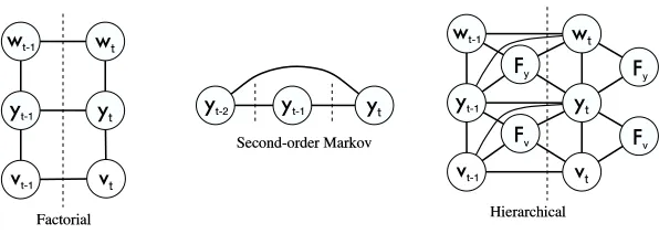
Figure 2: Examples of DCRFs. The dashed lines indicate the boundary between time steps. The input variables x are not shown.

fk(yt−1,yt,x,t)for each label transition. (Here we write the feature functions as potentially depend-ing on the entire input sequence.) Feature functions can be arbitrary. For example, a feature function fk(yt−1,yt,x,t)could be a binary test that has value 1 if and only if yt−1has the label “adjective”, yt has the label “proper noun”, and xt begins with a capital letter.

3. Dynamic CRFs

In this section, we define dynamic CRFs (Section 3.1) and describe methods for inference (Sec-tion 3.2) and parameter estima(Sec-tion (Sec(Sec-tion 3.3).

3.1 Model Representation

A dynamic CRF (DCRF) is a conditional distribution that factorizes according to an undirected graphical model whose structure and parameters are repeated over a sequence. As with a DBN, a DCRF can be specified by a template that gives the graphical structure, features, and weights for two time slices, which can then be unrolled given an input x. The same set of features and weights is used at each sequence position, so that the parameters are tied across the network. Several example templates are given in Figure 2.

Now we give a formal description of the unrolling process. Let y={y1. . .yT}be a sequence of random vectors yi= (yi1. . .yim),where yiis the state vector at time i, and yi jis the value of variable j at time i. To give the likelihood equation for arbitrary DCRFs, we require a way to describe a clique in the unrolled graph independent of its position in the sequence. For this purpose we introduce the concept of a clique index. Given a time t, we can denote any variable yi j in y by two integers: its index j in the state vector yi, and its time offset∆t=i−t. We will call a set c={(∆t,j)}of such pairs a clique index, which denotes a set of variables yt,cby yt,c≡ {yt+∆t,j|(∆t,j)∈c}. That is, yt,c is the set of variables in the unrolled version of clique index c at time t.

Now we can formally define DCRFs:

field if and only if

p(y|x) = 1

Z(x)

∏

_{t c}

∏

_∈Cexp

∑

_k λkfk(yt,c,x,t)

!

where Z(x) =∑y∏t∏c∈Cexp(∑kλkfk(yt,c,x,t))is the partition function.

Although we define a DCRF has having the same set of features for all of its cliques, in practice we choose each feature function fk so that it is non-zero only on cliques with some particular index ck. Thus, we will sometimes think of each clique index has having its own set of features and weights, and speak of fk andλk as having an associated clique index ck.

DCRFs generalize not only linear-chain CRFs, but more complicated structures as well. For example, in this paper, we use a factorial CRF (FCRF), which has linear chains of labels, with connections between cotemporal labels. We name these after factorial HMMs (Ghahramani and Jordan, 1997). Figure 1(b) shows an unrolled factorial CRF. Consider an FCRF with L chains, where Y`,t is the variable in chain`at time t. The clique indices for this DCRF are of the form {(0, `),(1, `)}for each of the within-chain edges and{(0, `),(0, `+1)} for each of the between-chain edges. The FCRF p defines a distribution over output variables as:

p(y|x) = 1 Z(x)

T−1

∏

t=1 L

∏

`=1

Φ`(y`,t,y`,t+1,x,t)

!

T

∏

t=1 L−1

∏

`=1

Ψ`(y`,t,y`+1,t,x,t)

!

,

where {Φ`} are the factors over the within-chain edges, {Ψ`} are the factors over the

between-chain edges, and Z(x)is the partition function. The factors are modeled using the features{fk}and weights{λk}of G as:

Φ`(y`,t,y`,t+1,x,t) =exp

(

∑

k

λkfk(y`,t,y`,t+1,x,t)

)

,

Ψ`(y`,t,y`+1,t,x,t) =exp

(

∑

k

λkfk(y`,t,y`+1,t,x,t)

)

.

More complicated structures are also possible, such as second-order CRFs, and hierarchical CRFs, which are moralized versions of the hierarchical HMMs of Fine et al. (1998).1 As in DBNs, this factorized structure can use many fewer parameters than the cross-product state space: even the two-level FCRF we discuss below uses less than an eighth of the parameters of the corresponding cross-product CRF.

3.2 Inference in DCRFs

Inference in a DCRF can be done using any inference algorithm for undirected models. For an unla-beled sequence x, we typically wish to solve two inference problems: (a) computing the marginals p(yt,c|x) over all cliques yt,c, and (b) computing the Viterbi decoding y∗=arg maxyp(y|x). The

Viterbi decoding can be used to label a new sequence, and marginal computation is used for param-eter estimation (Section 3.3).

If the number of states is not large, the simplest approach is to form a linear chain whose output space is the cross-product of the original DCRF outputs, and then perform forward-backward. In

other words, a DCRF can always be viewed as a linear-chain CRF whose feature functions take a special form, analogous to the relationship between generative DBNs and HMMs. The cross-product space is often very large, however, in which case this approach is infeasible. Alternatively, one can perform exact inference by applying the junction tree algorithm to the unrolled DCRF, or by using the special-purpose inference algorithms that have been designed for DBNs (Murphy, 2002), which can avoid storing the full unrolled graph.

In complex DCRFs, though, exact inference can still be expensive, making approximate meth-ods necessary. Furthermore, because marginal computation is needed during training, inference must be efficient so that we can use large training sets even if there are many labels. The largest experiment reported here required computing pairwise marginals in 866,792 different graphical models: one for each training example in each iteration of a convex optimization algorithm. In the remainder of the section, we describe approximate inference using loopy belief propagation (BP).

Although belief propagation is exact only in certain special cases, in practice it has been a successful approximate method for general graphical models (Murphy et al., 1999; Aji et al., 1998). For simplicity, we describe BP for a pairwise CRF with factors{Φ(xu,xv)}, but the algorithm can be generalized to arbitrary factor graphs. Belief propagation algorithms iteratively update a vector m= (mu(xv))of messages between pairs of vertices xuand xv. The update from xuto xvis given by:

mu(xv)←

∑

xu

Φ(xu,xv)

∏

xt6=xv

mt(xu), (1)

whereΦ(xu,xv)is the potential on the edge(xu,xv). Performing this update for one edge(xu,xv)in one direction is called sending a message from xu to xv. Given a message vector m, approximate marginals are computed as

p(xu,xv)←κΦ(xu,xv)

∏

xt6=xv

mt(xu)

∏

xw6=xu

mw(xv),

whereκis a normalization constant.

At each iteration of belief propagation, messages can be sent in any order, and choosing a good schedule can affect how quickly the algorithm converges. We describe two schedules for belief propagation: tree-based and random. The tree-based schedule, also known as tree reparameter-ization (TRP) (Wainwright et al., 2001; Wainwright, 2002), propagates messages along a set of cross-cutting spanning trees of the original graph. At each iteration of TRP, a spanning tree

T

(i)∈ϒ is selected, and messages are sent in both directions along every edge in

T

(i), which amounts to exact inference on

T

(i). In general, trees may be selected from any setϒ={

T

}as long as the trees inϒcover the edge set of the original graph. In practice, we select trees randomly, but we select first edges that have never been used in any previous iteration.

The random schedule simply sends messages across all edges in random order. To improve convergence, we arbitrarily order each edge ei= (si,ti) and send all messages msi(ti) before any

messages mti(si). Note that for a graph with V nodes and E edges, TRP sends O(V)messages per

BP iteration, while the random schedule sends O(E)messages.

An alternative to schedule is a synchronous schedule, in which conceptually all messages are sent at the same time. In the tree-based and random schedules, once a message is updated, its new values are immediately available for other messages. In the synchronous schedule, on the other hand, when computing a message m(uj)(xv)at iteration j of BP, the previous message values m(tj−1)(xu)are always used, even if an updated value m(

j)

results from the synchronous schedule in this paper, because preliminary experiments indicated that it requires many more iterations to converge than the other schedules.

Finally, dynamic schedules for BP (Elidan et al., 2006), which depend on the current message values during inference, have recently been shown to converge significantly faster than TRP on sufficiently difficult graphs, and may be preferable to TRP on certain DCRFs. We do not consider them in this paper, however.

To perform Viterbi decoding, we use the same propagation algorithms, except that the summa-tion in Equasumma-tion (1) is replaced by maximizasumma-tion.

3.3 Parameter Estimation in DCRFs

In this section, we discuss exact parameter estimation (Section 3.3.1) and approximate parameter estimation using belief propagation (Section 3.3.2). Also, we introduce a novel approximate training procedure called cascaded training (Section 3.3.3).

3.3.1 EXACT PARAMETERESTIMATION

The parameter estimation problem is to find a set of parametersΛ={λk}given training data

D

= {x(i)_,y(i)_}N

i=1. More specifically, we optimize the conditional log-likelihood

L

(Λ) =

∑

i

log pΛ(y(i)|x(i)).

The derivative of this with respect to a parameterλk associated with clique index c is

∂L

∂λk =

∑

_i

∑

_t fk(yt(,ic),x(i),t) −

∑

i

∑

t

∑

yt,c

p_Λ(yt,c|x(i))fk(yt,c,x(i),t).

(2)

where yt(,ic)is the assignment to yt,cin y(i), and yt,cranges over assignments to the clique c. Observe that it is the factor pΛ(yt,c |x(i))that requires us to compute marginal probabilities in the unrolled DCRF.

To reduce overfitting, we define a prior p(Λ) over parameters, and optimize log p(Λ|

D

) =

L

(Λ)+log p(Λ). We use a spherical Gaussian prior with mean µ=0 and covariance matrixΣ=σ2_I, so that the gradient becomes

∂p(Λ|

D

)

∂λk =∂λk∂L − λk σ2.

This corresponds to optimizing

L

(Λ)using`2regularization. Other priors are possible, for example, an exponential prior, which corresponds to regularizing

L

(Λ)by an`1norm.

approximation to the Hessian using only the gradient. But standard quasi-Newton methods, such as BFGS, also approximate the Hessian by a full K×K matrix, which is too large. Therefore, we use a limited-memory version of BFGS, called L-BFGS (Nocedal and Wright, 1999), which approxi-mates the Hessian in such a way that the full K×K matrix is never calculated explicitly. L-BFGS has previously been shown to outperform other optimization algorithms for linear-chain CRFs (Sha and Pereira, 2003; Malouf, 2002; Wallach, 2002). In particular, iterative scaling algorithms such as GIS and IIS have been shown to be much slower than gradient-based algorithms such as L-BFGS or preconditioned conjugate gradient.

All of the methods we have described are batch methods, meaning that they examine all of the training data before making a gradient update. Recently, stochastic gradient methods, which make gradient updates based on small subsets of the data, have been shown to converge significantly faster for linear-chain CRFs (Vishwanathan et al., 2006). It is likely that stochastic gradient methods would perform similarly well for DCRFs, but we do not use them in the experiments reported here. The discussion above was for the fully-observed case, where the training data include observed values for all variables in the model. If some nodes are unobserved, the optimization problem becomes more difficult, because the log likelihood is no longer convex in general. We describe this case in Section 3.4.1.

3.3.2 APPROXIMATEPARAMETERESTIMATIONUSINGBP

For models in which exact inference is infeasible, we use approximate inference during training. In Section 3.2, we discussed inference in DCRFs. In this section, we discuss additional issues that arise when using BP during training. First, to simplify notation in this section, we will write a DCRF as p(y|x) =Z(x)−1_∏t∏cψt

,c(yt,c), where each factor in the unrolled DCRF is defined as

ψt,c(yt,c) =exp

(

∑

k

λkfk(yt,c,x,t)

)

.

That is, we drop the dependence of the factors{ψt,c}on x.

For approximate parameter estimation, the basic procedure is to optimize using the gradient (2) as described in the last section, but instead of running an exact inference algorithm on each training example to obtain marginal distributions p_Λ(yt,c | x(i)), we run BP on each training instance to obtain approximate factor beliefs bt,c(yt,c)for each clique yt,cand approximate node beliefs bs(ys) for each output variable s.

Now, although BP provides approximate marginal distributions that allow calculating the gra-dient, there is still the issue of how to calculate an approximate likelihood. In particular, we need an approximate objective function whose gradient is equal to the approximate gradient we have just described. We use the approximate likelihood

ˆ

`(Λ;{b}) =

∑

i log

"

∏t∏cbt,c(y(t,ic)) ∏sbs(y(si))ds−1

#

, (3)

BP can be viewed as attempting to solve an optimization problem over possible choices of marginal distributions, for a particular cost function called the Bethe free energy. More techni-cally, it has been shown that fixed points of BP are stationary points of the Bethe free energy (for more details, see Yedidia et al., 2005), when minimized over locally-consistent beliefs. The Bethe energy is an approximation to another cost function, which Yedidia et al. call the Helmholtz free energy. Since the minimum Helmhotlz energy is exactly−log Z(x), we approximate−log Z(x)by the minimizing value of the Bethe energy, that is:

`BETHE(Λ) =

∑

i

∑

t

∑

c

logψt,c(yt,c) +

∑

i

min

{b}

F

BETHE(b), (4)

where

F

BETHEis the Bethe free energy, which is defined as

F

BETHE(b) =

∑

t

∑

c

∑

yt,c

bt,c(yt,c)log

bt,c(yt,c) ψt,c(yt,c)

−

∑

s

(ds−1)

∑

xs

bs(ys)log bs(ys).

So approximate training with BP can be viewed as solving a saddlepoint problem of maximizing

`BETHE with respect to the model parameters and minimizing with respect to the beliefs bt,c(yt,c).

Approximate training using BP is just coordinate ascent: BP optimizes`BETHE with respect to b for

fixed Λ; and a step along the gradient (2) optimizes `BETHE with respect to Λ for fixed b. Taking

the partial derivative of (4) with respect to a weightλk, we obtain the gradient (2) with marginal distributions replaced by beliefs, as desired.

To justify the approximate likelihood (3), we note that the Bethe free energy can be written a dual form, in which the variables are interpreted as log messages rather than beliefs. Details of this are presented by Minka (2001a, 2005). Substituting the Bethe dual problem into (4) and simplifying yields (3).

3.3.3 CASCADEDPARAMETERESTIMATION

Joint maximum likelihood training assumes that we have access to data in which we have observed all of the variables. Sometimes this is not the case. One example is transfer learning, which is the general problem of using previous learning problems that a system has seen to aid its learning of new, related tasks. Usually in transfer learning, we have one data set labeled with the old task variables and one with the new task variables, but no data that is jointly labeled. In this section, we describe a cascaded parameter estimation procedure that can be applied when the data is not fully labeled.

For a factorial CRF with N levels, the basic idea is to train each level separately as if it were a linear-chain CRF, using the single-best prediction of the previous level as a feature. At the end, each set of individually-trained weights defines a pair of factors, which are simply multiplied together to form the full FCRF. The cascaded procedure is described formally in Algorithm 1. In this de-scription, the two clique indices for each level`of the FCRF are denoted by cW

` for the within-level

cliques, with features fW

`,k(y`t,yt`+1,x,t)and weightsΛ

W

`; and another index cP`for the between-level

cliques, with features fP

`,k(y`t,yt`−1,x,t)and weightsΛP`.

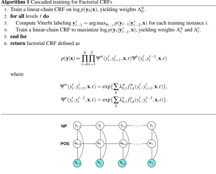
Algorithm 1 Cascaded training for Factorial CRFs

1: Train a linear-chain CRF on log p(y0|x), yielding weightsΛW

0. 2: for all levels`do

3: Compute Viterbi labeling y∗<sub>`−1</sub>=arg maxy`−1p(y`−1|y

∗

`−2,x)for each training instance i. 4: Train a linear-chain CRF to maximize log p(y`|y∗`−1,x), yielding weightsΛW` andΛP`.

5: end for

6: return factorial CRF defined as

p(y|x)∝

N

∏

`=0

T

∏

t=1 ΨW₍

y`<sub>t</sub>,y`_t+1,x,t)ΨP₍

y`<sub>t</sub>,y`_t−1,x,t)

where

ΨW

(y_t`,y`_t+1,x,t) =exp{

∑

k

λW

k,`f

W

`,k(yt`,yt`+1,x,t)}, ΨP

(y`<sub>t</sub>,y`_t−1,x,t) =exp{

∑

k

λP

k,`f`,Pk(yt`,y`t−1,x,t)}.

t T

. . . . . .

NP

POS

t−1 t t+1 T

t−1 t+1

t+1

t−1 t T

X X X X

y y y y

w w w w

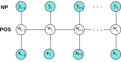
Figure 3: Graphical representation of factorial CRF for the joint noun phrase chunking and part-of-speech tagging problem, where the chain y represents the NP labels, and the chain w represents the POS labels.

3.4 Marginal DCRFs

3.4.1 MARGINALDCRFS,ANDPARAMETERESTIMATION

First, we define the marginal DCRF model.

Definition 2 A distribution p is a marginal DCRF over random vectors(y,w)given inputs x if it can be written as:

p_Λ(y|x) =

∑

w

p_Λ(y,w|x),

where pΛ(y,w|x)is a DCRF.

Parameter estimation proceeds by optimizing the log likelihood

L

(Λ) =

∑

i

log pΛ(y(i)|x(i)) =

∑

i

log

∑

w

pΛ(y(i),w|x(i)). (5)

Intuitively, this objective function concentrates on the conditional likelihood over the variables y, possibly sacrificing accuracy on the variables w. Indeed, this objective function ignores any observations of w in the training set. We can take these observations into account in some partial way by careful choice of initialization, as we describe in Section 4.3.

The derivative of (5) with respect to a parameterλk associated with a clique index c is:

∂L(Λ)

∂λk =

∑

_i

∑

_{t w}

∑

_˜t,cp(w˜t,c|y(i),x(i))fk(y(t,ic),w˜t,c,x(t,i)c)−

∑

i

∑

t ˜yt,

∑

c,w˜t,c

p(˜yt,c,w˜t,c|x(i))fk(˜yt,c,w˜t,c,x(i)), (6)

where y(_t,i_c)is the subset of the training vector y(i) _{that occurs in clique c instantiated at time t; the}

summation over ˜yt,cranges over all assignments to clique c; and wt,cand ˜wt,care defined similarly. Also, to reduce overfitting, we include a prior on parameters, as in Section 3.3.

Another way to understand the gradient is as follows. For any function f(λ), we have

∂f

∂λ =f(λ) ∂log f

∂λ ,

which can be seen by applying the chain rule to log f and rearranging. Applying this to the marginal likelihood`(Λ) =log∑_wp(y,w|x), we get

∂`

∂λk =

1

∑wp(y,w|x)

∑

w

∂ ∂λk

p(y,w|x)

= 1

p(y|x)

∑

_w p(y,w|x)

∂ ∂λk

log p(y,w|x)

=

∑

w

p(w|y,x) ∂

∂λk

log p(y,w|x)

,

which is the expectation of the fully-observed gradient over all the unobserved variables. Substitut-ing the expression (2) for the fully-observed gradient yields (6).

. . . . . .

NP

POS

t−1 t t+1 T

t−1

t−1

X t t+1 _T

t+1

t _T

X

X X

y y y y

w w w w

Figure 4: Graphical representation of factorial CRF for the joint noun phrase chunking and part of speech labeling problem, demonstrating the process for computing the probability p(w|y(i)_,x(i)_).

optimization algorithms can be used, such as expectation maximization and its variants. Unfortu-nately, unlike the fully-observed case, the penalized likelihood for marginal DCRFs is not convex in general. Thus standard optimization techniques are guaranteed to find only a local maximum, the quality of which depends on where in parameter space the optimizer is initialized. In Section 4.3, we evaluate an approach for finding a good starting point.

3.4.2 INFERENCE INMARGINALDCRFS

In this section, we discuss how to compute the model probabilities required by the marginal DCRF gradient. The solutions are very similar to those for DCRFs. The gradient in Equation (6) requires computing two kinds of marginal probabilities. First, the marginal probabilities p(˜yt,c,w˜t,c|x(i))in the second term can be computed by standard inference algorithms, just as in Section 3.2. Second, the other kind of marginal probabilities are of the form p(w˜t,c|y(i),x(i)), used in the first term on the right hand side of Equation (6). We do this by performing inference in a clamped model, in which y is fixed to its observed values (shown in Figure 4). More specifically, to form the clamped model for a training instance {x(i)_,y(i)_,w(i)_{}, we instantiate y}

t nodes (nodes associated with the noun phrase labels) from y(i). This eliminates the edges that are solely between yt nodes, and hence p(w|y(i)_,x(i)_{)can be computed efficiently using any inference algorithm. Finally, to compute the}

actual likelihood (5), we can pick an arbitrary assignment w0and compute the likelihood p(y|x) = p(y,w0|x)/p(w0|y,x).

For decoding in marginal DCRFs, we wish to find the most likely label sequence for only the y variables, that is:

y∗=arg max

y p(y|x)

=arg max

y

∑

_w p(y,w|x).

(7)

Algorithm 2 MAP algorithm for marginal FCRF

1 If u is a marginalized node, perform: mu(xv)←∑xu{Φ(xu,xv)∏xt6=xvmt(xu)}.

2 If u is not a marginalized node, perform: mu(xv)←maxxu{Φ(xu,xv)∏xt6=xvmt(xu)}.

3 For all nodes perform: p(xu,xv)←κΦ(xu,xv)∏xt6=xvmt(xu)∏xw=6 xumw(xv).

200 300 400 500 600 700 800 900

84

86

88

90

Number of training instances

F1 on NP chunks

FCRF CRF+CRF

Figure 5: Performance of FCRFs and cascaded approaches on noun-phrase chunking, averaged over five repetitions. The error bars on FCRF and CRF+CRF indicate the range of the repetitions.

Finally, an important point is that part of the reason that the marginal maximization in (7) is possible in our setting is because of our choice of w. In the application considered here, w is a single chain of a two-chain FCRF, so that the marginal p(y|x)is likewise the marginal of a single chain, which can be approximated by BP in a natural way. In a more difficult case—for example, if the variables y are disconnected, spread throughout the model, and highly correlated—further approximation would be necessary.

4. Experiments

We present experiments comparing factorial CRFs to other approaches on noun-phrase chunking (Sang and Buchholz, 2000). Also, we compare different schedules of loopy belief propagation in factorial CRFs.

4.1 FCRFs for Noun-Phrase Chunking

Size CRF+CRF Brill+CRF FCRF

223 86.23 93.12

447 90.44 95.43

POS accuracy 670 92.33 N/A 96.34

894 93.56 96.85

2234 96.18 97.87

8936 98.28 98.92

223 81.92 89.19

447 86.58 91.85

Joint accuracy 670 88.68 N/A 92.86

894 90.06 93.60

2234 93.00 94.90

8936 95.56 96.48

223 83.84 86.02 86.03 447 86.87 88.56 88.59 NP F1 670 88.19 89.65 89.64 894 89.21 90.31 90.55 2234 91.07 91.90 92.02 8936 93.10 93.33 93.87

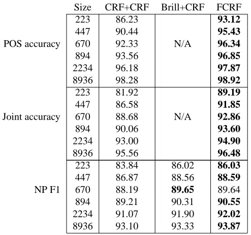
Table 1: Comparison of performance of cascaded models and FCRFs on simultaneous noun-phrase chunking and POS tagging. The column Size lists the number of sentences used in training. The row CRF+CRF lists results from cascaded CRFs, and Brill+CRF lists results from a linear-chain CRF given POS tags from the Brill tagger. The FCRF always outperforms CRF+CRF, and given sufficient training data outperforms Brill+CRF. With small amounts of training data, Brill+CRF and the FCRF perform comparably, but the Brill tagger was trained on over 40,000 sentences, including some in the CoNLL 2000 test set.

Marcus, 1995). The task is typically performed by an initial pass of part-of-speech tagging, but then it can be difficult to recover from errors by the tagger. In this section, we address this problem by performing part-of-speech tagging and noun-phrase segmentation jointly in a single factorial CRF.

Our data comes from the CoNLL 2000 shared task (Sang and Buchholz, 2000), and consists of sentences from the Wall Street Journal annotated by the Penn Treebank project (Marcus et al., 1993). We consider each sentence to be a training instance, with single words as tokens. The data are divided into a standard training set of 8936 sentences and a test set of 2012 sentences. There are 45 different POS labels, and the three NP labels.2

We compare a factorial CRF to two cascaded approaches, which we call CRF+CRF and Brill+ CRF. CRF+CRF uses one linear-chain CRF to predict POS labels, and another linear-chain CRF to predict NP labels, using as a feature the Viterbi POS labeling from the first CRF. Brill+CRF predicts NP labels using the POS labels provided from the Brill tagger, which we expect to be more accurate than those from our CRF, because the Brill tagger was trained on over four times more data, including sentences from the CoNLL 2000 test set.

The factorial CRF uses the graph structure in Figure 1(b), with one chain modeling the part-of-speech process and the other modeling the noun-phrase process. We use L-BFGS to optimize the

wt−δ=w

wt matches[A-Z][a-z]+ wt matches[A-Z] wt matches[A-Z]+

wt matches[A-Z]+[a-z]+[A-Z]+[a-z]

wt matches.*[0-9].*

wt appears in list of first names, last names, company names, days, months, or geographic entities wt is contained in a lexicon of words

with POS T (from Brill tagger) Tt=T

qk(x,t+δ)for all k andδ∈[−3,3]

Table 2: Input features qk(x,t)for the CoNLL data. In the above wt is the word at position t, Tt is the POS tag at position t, w ranges over all words in the training data, and T ranges over all part-of-speech tags.

posterior p(Λ|

D

), and TRP to compute the marginal probabilities required by∂L/∂λk. Based on past experience with linear-chain CRFs, we use the prior varianceσ2=10 for all models.

We factorize our features as fk(yt,c,x,t) =pk(yt,c)qk(x,t)where pk(yt,c)is a binary function on the assignment, and qk(x,t) is a function solely of the input string. Table 2 shows the features we use. All three approaches use the same features, with the obvious exception that the FCRF and the first stage of CRF+CRF do not use the POS features Tt =T .

Performance on noun-phrase chunking is summarized in Table 1. As usual, we measure per-formance on chunking by precision, the percentage of returned phrases that are correct; recall, the percentage of correct phrases that were returned; and their harmonic mean F1. In addition, we also report accuracy on POS labels,3and joint accuracy on (POS, NP) pairs. Joint accuracy is simply the number of sequence positions for which all labels were correct.

Each row in Table 1 is the average of five different random subsets of the training data, except for row 8936, which is run on the single official CoNLL training set. All conditions used the same 2012 sentences in the official test set.

On the full training set, FCRFs perform better on NP chunking than either of the cascaded approaches, including Brill+POS. The Brill tagger (Brill, 1994) is an established part-of-speech tagger whose training set is not only over four times bigger than the CoNLL 2000 data set, but also includes the WSJ corpus from which the CoNLL 2000 test set was derived. The Brill tagger is 97% accurate on the CoNLL data. Also, note that the FCRF—which predicts both noun-phrase boundaries and POS—is more accurate than a linear-chain CRF which predicts only part of speech. Our explanation for this is that the NP chain captures long-run dependencies among the POS labels. The POS-only accuracy is listed under CRF+CRF in Table 1.

Method Time (hr) NP F1 LBFGS iter

µ s µ s µ

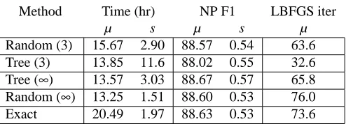
Random (3) 15.67 2.90 88.57 0.54 63.6 Tree (3) 13.85 11.6 88.02 0.55 32.6 Tree (∞) 13.57 3.03 88.67 0.57 65.8 Random (∞) 13.25 1.51 88.60 0.53 76.0 Exact 20.49 1.97 88.63 0.53 73.6

Table 3: Comparison of F1 performance on the chunking task by inference algorithm. The columns labeled µ give the mean over five repetitions, and s the sample standard deviation. Ap-proximate inference methods have labeling accuracy very similar to exact inference with lower total training time. The differences in training time between Tree (∞) and Ex-act and between Random (∞) and Exact are statistically significant by a paired t-test (d f =4; p<0.005).

On smaller training subsets, the FCRF outperforms CRF+CRF and performs comparably to Brill+CRF. For all the training subset sizes, the difference between CRF+CRF and the FCRF is statistically significant by a two-sample t-test (p<0.002). In fact, there was no subset of the data on which CRF+CRF performed better than the FCRF. The variation over the randomly selected training subsets is small—the standard deviation over the five repetitions has mean 0.39—indicating that the observed improvement is not due to chance. Performance and variance on noun-phrase chunking is shown in Figure 5.

On this data set, several systems are statistically tied for best performance. Kudo and Matsumoto (2001) report an F1 of 94.39 using a combination of voting support vector machines. Sha and Pereira (2003) give a linear-chain CRF that achieves an F1 of 94.38, using a second-order Markov assumption, and including bigram and trigram POS tags as features. An FCRF imposes a first-order Markov assumption over labels, and represents dependencies only between cotemporal POS and NP label, not POS bigrams or trigrams. Thus, Sha and Pereira’s results suggest that more richly-structured DCRFs could achieve better performance than an FCRF.

Other DCRF structures can be applied to many different language tasks, including informa-tion extracinforma-tion. Peshkin and Pfeffer (2003) apply a generative DBN to extracinforma-tion from seminar announcements (Frietag and McCallum, 1999), attaining improved results, especially in extracting locations and speakers, by adding a factor to remember the identity of the last non-background label.

4.2 Comparison of Inference Algorithms

Because DCRFs can have rich graphical structure, and require many marginal computations during training, inference is critical to efficient training with many labels and large data sets. In this section, we compare different inference methods both on training time and labeling accuracy of the final model.

We train factorial CRFs on the noun-phrase chunking task described in the last section. We compute the gradient using exact inference and approximate belief propagation using both random and tree-based schedules, as described in Section 3.2. Algorithms are considered to have converged when no message changes by more than 10−3. In these experiments, we observe that the approxi-mate BP algorithms always converge, although this is not guaranteed in general. We train on five random subsets of 5% of the training data, and the same five subsets are used in each condition. All experiments were performed on a 2.8 GHz Intel Xeon with 4 GB of memory.

In an attempt to reduce the training time, we also examine early stopping of BP. For each message-passing schedule, we compare terminating belief propagation on convergence (Random(∞) and Tree(∞) in Table 3), to terminating after three iterations (Random (3) and Tree (3)). In all cases, we run BFGS to convergence. To be clear, training as a whole is a two-loop process: in the outer loop, BFGS updates the parameters to increase the likelihood, and in the inner loop, belief prop-agation passes messages to compute beliefs which are used to approximate the gradient. In these experiments, we examine early stopping in the inner loop, not the outer loop.

Thus, early-stopping of BP need not lead to faster training time overall. Of course each call the inner loop of training becomes faster with early stopping. However, early stopping of BP can interact badly with the outer loop, because it makes the gradients less accurate. If the gradient is too inaccurate, then the outer loop will require many more iterations, resulting in greater training time overall, even though the time per gradient computation is lower. Another hazard is that no maximizing step may be possible along the approximate gradient, even if one is possible along the true gradient. When that happens, the gradient descent algorithm terminates prematurely, leading to decreased performance.

Table 3 shows the average F1 score and total training times of DCRFs trained by the different inference methods. Unexpectedly, letting the belief propagation algorithms run to convergence led to lower training time than the early cutoff. For example, even though Random(3) averaged 427 sec per gradient computation compared to 571 sec for Random(∞), Random(∞) took less total time to train, because Random(∞) needed an average of 83.6 gradient computations per training run, compared to 133.2 for Random(3).

As for final classification performance, the various approximate methods and exact inference perform similarly, except that Tree(3) has lower final performance because maximization ended prematurely, averaging only 32.6 maximizer iterations. The variance in F1 over the subsets, al-though not large, is much larger than the F1 difference between the inference algorithms.

Previous work (Wainwright, 2002) has shown that TRP converges faster than synchronous be-lief propagation, that is, with Jacobi updates. Both the schedules discussed in Section 3.2 use asynchronous Gauss-Seidel updates. We emphasize that the graphical models in these experiments are always pairs of coupled chains. On more complicated models, or with a different choice of span-ning trees, tree-based updates could outperform random asynchronous updates. Also, in complex models, the difference in classification accuracy between exact and approximate inference could be larger, but then exact inference is likely to be intractable.

Initial model Precision Recall Accuracy F1

Joint FCRF Random 0.431 0.420 0.710 0.425

Random 0.470 0.430 0.730 0.450

1-Joint 0.470 0.430 0.730 0.450

5-Joint 0.460 0.418 0.726 0.440

10-Joint 0.460 0.418 0.730 0.440

Marginal FCRF 15-Joint 0.454 0.415 0.725 0.434

20-Joint 0.460 0.423 0.730 0.440

25-Joint 0.453 0.408 0.725 0.430

Final-Joint 0.477 0.404 0.723 0.437

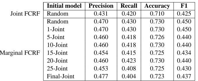
Table 4: NP chunking results comparing marginal FCRF and jointly trained FCRF performance using a data set consisting of 21 training instances and 195 testing instances.

Third, running belief propagation to convergence leads both to increased classification accuracy and lower overall training time than an early cutoff.

4.3 Experiments with Marginal FCRFs

In this section we apply marginal DCRFs (Section 3.4) to the CoNLL 2000 shared task data set (Sang and Buchholz, 2000), and to synthetic data.

4.3.1 NOUN-PHRASECHUNKING

In Section 4.1 we presented experiments using FCRFs for the noun-phrase segmentation problem. In this section we apply marginal FCRFs to the same problem, where we wish to predict the noun-phrase labels and marginalize out the part-of-speech labels.

Because the marginal likelihood is not a convex function of the model parameters, our choice of initialization can affect the quality of the learned model. In order to partly capture the usefulness of the part-of-speech labels in the data, we initialize the marginal FCRF from a joint FCRF at some intermediate stages of training. We train an FCRF using the joint likelihood from a random initialization, saving the model parameters after each iteration of BFGS. Then we use each of those saved parameter settings as an initialization for marginal training; we call this n-joint initialization, where n is the number of BFGS steps on the joint likelihood used for the initializer. We compare this to initializing from a fully-trained joint FCRF (Final-Joint) and and to initializing from random parameters. We use two different-sized subsets of the CoNLL 2000 data. The first subset contains 21 training instances and 195 testing instances (Table 4). The second contains 447 training instances and 2012 testing instances (Table 5).

Initial model Precision Recall Accuracy F1

Joint FCRF Random 0.819 0.803 0.913 0.811

Random 0.814 0.800 0.910 0.806

1-Joint 0.810 0.800 0.910 0.810

5-Joint 0.810 0.800 0.909 0.806

20-Joint 0.810 0.782 0.907 0.795

30-Joint 0.820 0.791 0.908 0.804

Marginal FCRF 50-Joint 0.820 0.800 0.913 0.808

70-Joint 0.820 0.800 0.913 0.810

80-Joint 0.827 0.800 0.920 0.813

90-Joint 0.827 0.800 0.920 0.814

Final-Joint 0.825 0.797 0.913 0.811

Table 5: NP chunking results comparing marginal FCRF and jointly trained FCRF performance using a data set consisting of 447 training instances and 2012 testing instances.

t−1

t−1

X

W

Y

Xt t

t−1 t

w

y w

y

Figure 6: Graphical representation of the DBN used for generating synthetic data.

4.3.2 SYNTHETICDATA

In this section we discuss a set of experiments with synthetic data that further highlights the dif-ferences between joint and marginal DCRFs. In this set of experiments we generate synthetic data using randomly chosen generative models that all share the graphical structure shown in Figure 6. All variables take on discrete values from a finite domain of cardinality five. The parameters (hor-izontal and vertical transition probability matrices, and also the observation model) are randomly selected from a uniform Dirichlet distribution with parameter µ=0.5. We then sample each model to generate a set of 200 training sequences and 400 testing sequences, each of length 20.

0 0.2 0.4 0.6 0.8 1

0 0.2 0.4 0.6 0.8 1

Marginal Accuracy

Joint Accuracy

Figure 7: Accuracy of the marginal FCRF versus accuracy of the joint FCRF over the factor Y. Each point represents a training and testing set generated from a different randomly-selected generative model with structure shown in Figure 6.

If the joint FCRF performs well, however, the marginal FCRF tends to yield the same prediction accuracy. We conjecture that when we have learned a good joint FCRF model given a set of training sequences, the marginally trained FCRF initialized by the joint FCRF does not offer improvement in accuracy. However, when the joint FCRF performs poorly, we can train a marginal FCRF that is likely to outperform the joint FCRF.

In order to further study this phenomenon, we measure the entropy of the model distribution, the idea being that when the model is very accurate, it has little uncertainty over the latent variables, so modeling the marginal directly is unlikely to make a difference. To measure the uncertainty over output labels, we use a per-timestep entropy measure, that is,∑i∑tH(p(yt|x(i))), where as before i ranges over test instances, and t over sequence positions. Figure 8 shows the plot of the accuracy of the joint FCRF versus its per-timestep entropy. As the per-timestep entropy of the model increases, the accuracy decreases. This suggests that the per-timestep entropy can serve as a surrogate measure to decide which problems are most appropriate for marginal training.

0 0.2 0.4 0.6 0.8 1

0 0.2 0.4 0.6 0.8 1 1.2 1.4 1.6 1.8

Joint Accuracy

Mean Entropy

Figure 8: Accuracy of the joint FCRF as a function of the mean per-timestep entropy, E(H(p(yt|x))), averaged over all time steps t, and all testing sequences x(i), of the joint FCRF.

0 0.5 1 1.5 2 2.5 3

0 0.5 1 1.5 2

Marginal Accuracy / Joint Accuracy

Mean Entropy

Figure 9: Ratio of the accuracy of the marginal FCRF accuracy to the the joint FCRF accuracy, as a function of the mean per-timestep entropy of the joint FCRF.

4.4 Cascaded Training for Transfer Learning

wt=w

wt matches[A-Z][a-z]+ wt matches[A-Z][A-Z]+ wt matches[A-Z] wt matches[A-Z]+

wt matches[A-Z]+[a-z]+[A-Z]+[a-z] wt appears in list of first names,

last names, honorifics, etc.

wt appears to be part of a time followed by a dash wt appears to be part of a time preceded by a dash wt appears to be part of a date

Tt=T

qk(x,t+δ)for all k andδ∈[−4,4]

Table 6: Input features qk(x,t)for the seminars data. In the above wt is the word at position t, Tt is the POS tag at position t, w ranges over all words in the training data, and T ranges over all Penn Treebank part-of-speech tags. The “appears to be” features are based on hand-designed regular expressions that can span several tokens.

System stime etime location speaker overall

WHISK Soderland (1999) 92.6 86.1 66.6 18.3 65.9

SRV Freitag (1998) 98.5 77.9 72.7 56.3 76.4

HMM Frietag and McCallum (1999) 98.5 62.1 78.6 76.6 78.9 RAPIER Califf and Mooney (1999) 95.9 94.6 73.4 53.1 79.3 SNOW-IE Roth and Wen-tau Yih (2001) 99.6 96.3 75.2 73.8 86.2

(LP)2 _{Ciravegna (2001) 99.0 95.5 75.0 77.6 86.8}

CRF (no transfer) This paper 99.1 97.3 81.0 73.7 87.8 FCRF (cascaded) This paper 99.2 96.0 84.3 74.2 88.4

FCRF (joint) This paper 99.1 96.0 85.3 76.3 89.2

Table 7: Comparison of F1performance on the seminars data. Joint decoding performs significantly better than cascaded decoding. The overall column is the mean of the other four. (This table was adapted from Peshkin and Pfeffer (2003).)

the messages are written by many different people, who each have different ways of presenting the announcement information.

Because the task includes finding locations and person names, the output of a named-entity tagger is a useful feature. It is not a perfectly indicative feature, however, because many other kinds of person names appear in seminar announcements—for example, names of faculty hosts, departmental secretaries, and sponsors of lecture series. For example, the token Host: indicates strongly that what follows is a person name, but that person is not the seminar’s speaker.

Figure 10: Learning curves for the seminars data set on the speaker field, averaged over 10-fold cross validation. Joint training performs equivalently to cascaded decoding with 25% more data.

procedure in Section 3.3.3. We are interested in two comparisons: (a) between the FCRF trained to incorporate transfer and a comparable linear-chain CRF, and (b) at test time, between cascaded decoding or joint decoding. By cascaded decoding, we mean an analogous procedure to cascaded training, in which the maximum-value assignment to the first level of the DCRF is computed without reference to the second level, then this assignment is clamped and decoding proceeds in the second level only. By joint decoding, we mean standard max-product inference in the full FCRF. We might expect joint decoding to perform better because of helpful feedback between the tasks: Information from the seminar-field predictions can improve named-entity predictions, which in turn improve the seminar-field predictions.

We use the predictions from a CRF named-entity tagger that we train on the standard CoNLL 2003 English data set. The CoNLL 2003 data set consists of newswire articles from Reuters labeled as either people, locations, organizations, or miscellaneous entities. It is much larger than the semi-nar announcements data set. While the named-entity data contains 203,621 tokens for training, the seminar announcements data set contains only slightly over 60,000 training tokens.

Previous work on the seminars data has used a one-field-per-document evaluation. That is, for each field, the CRF selects a single field value from its Viterbi path, and this extraction is counted as correct if it exactly matches any of the true field mentions in the document. We compute precision and recall following this convention, and report their harmonic mean F1. As in the previous work, we use 10-fold cross validation with a 50/50 training/test split. We use a spherical Gaussian prior on parameters with varianceσ2=0.5.

We evaluate whether joint decoding with cascaded training performs better than cascaded train-ing and decodtrain-ing. Table 7 compares cascaded and joint decodtrain-ing for CRFs with other previous results from the literature.4 The features we use are listed in Table 6. Although previous work has 4. We omit one relevant paper (Peshkin and Pfeffer, 2003) because its evaluation method differs from all the other

used very different feature sets from ours, all of our models use exactly the same features, including the no-transfer CRF baseline.

On the most challenging fields, locationandspeaker, cascaded transfer is more accurate than no transfer at all, and joint decoding is more accurate than cascaded decoding. In particular, for speaker, we see an error reduction of 8% by using joint decoding over cascaded. The difference in F1 between cascaded and joint decoding is statistically significant forspeaker(paired t-test; p = 0.017) but only marginally significant forlocation(p = 0.067). Our results are competitive with previous work; for example, onlocation, the CRF is more accurate than any of the existing systems, and the CRF has the highest overall performance, that is, averaged over all fields, than the previously reported systems.

Figure 10 shows the difference in performance between joint and cascaded decoding as a func-tion of training set size. Cascaded decoding with the full training set of 242 emails performs equiv-alently to joint decoding on only 181 training instances, a 25% reduction in the training set.

Examining the trained models, we can observe errors made by the general-purpose named entity tagger, and how they can be corrected by considering the seminars labels. In newswire text, long runs of capitalized words are rare, often indicating the name of an entity. In email announcements, runs of capitalized words are common in formatted text blocks like:

Location: Baker Hall

Host: Michael Erdmann

In this type of situation, the general named entity tagger often mistakes Host: for the name of an entity, especially because the word preceding Host is also capitalized. On one of the cross-validated testing sets, of 80 occurrences of the word Host:, the named-entity tagger labels 52 as some kind of entity. When joint decoding is used, however, only 20 occurrences are labeled as entities. Recall that in both of these settings, training is performed in exactly the same way; the only difference is that joint decoding takes into account information about the seminar labels when choosing named-entity labels. This is an example of how domain-specific information from the main task can improve performance on a more standard, general-purpose subtask.

5. Related Work

Since the original work on conditional random fields (Lafferty et al., 2001), there has been much interest in training discriminative models with more general graphical structures. One of the first such applications was relational Markov networks (Taskar et al., 2002), which were first applied to collective classification of Web pages. There has also been interest in grid-structured loopy CRFs for computer vision (He et al., 2004; Kumar and Hebert, 2003), in which jointly-trained Markov random fields are a classical technique. Another type of structured problem which has seen some attention in the literature is discriminative learning of distributions over context-free parse trees, in which training has done done using max-margin methods (Taskar et al., 2004b; McDonald et al., 2005) and perceptron-like methods (Viola and Narasimhan, 2005).

trained using EM (McCallum et al., 2005), which is described in general in Sutton and McCallum (2006). Latent-variable CRFs are closely related to neural networks, and many training techniques from that literature can be applied here.

Currently, the most popular alternative approaches to training structured discriminative models are maximum-margin training (Taskar et al., 2004a; Altun et al., 2003), and perceptron training (Collins, 2002), which has been especially popular in NLP because of its ease of implementation.

The factorial CRF that we present here should not be confused with the factorial Markov random fields that have been proposed in the computer vision community (Kim and Zabih, 2002). In that model, each of the factors is a grid, rather than a chain, and they interact through a directed model, as in a factorial HMM.

The DCRF application to transfer learning in Section 4.4 is reminiscent of stacking (Wolpert, 1992). The most notable difference is that because the levels are decoded jointly, information from later levels can affect the decisions made about earlier ones.

Finally, some results presented here have appeared in earlier conference versions, in particular the results on noun-phrase chunking (Sutton et al., 2004) and transfer learning (Sutton and McCal-lum, 2005).

6. Conclusions

Dynamic CRFs are conditionally-trained undirected sequence models with repeated graphical struc-ture and tied parameters. They combine the best of both conditional random fields and the widely successful dynamic Bayesian networks (DBNs). DCRFs address difficulties both of DBNs, by eas-ily incorporating arbitrary overlapping input features, and of previous conditional models, by allow-ing more complex dependence between labels. Inference in DCRFs can be done usallow-ing approximate methods, and training can be done by maximum a posteriori estimation.

Empirically, we have shown that factorial CRFs can be used to jointly perform several labeling tasks at once, sharing information between them. Such a joint model performs better than a model that does the individual labeling tasks sequentially, and has potentially many practical implications, because cascaded models are ubiquitous in NLP. Also, we have shown that using approximate in-ference leads to lower total training time with no loss in accuracy.

In future research, we plan to explore other inference methods to make training more efficient, including expectation propagation (Minka, 2001b), contrastive divergence (Hinton, 2002) and vari-ational approximations. Finally, investigating other DCRF structures, such as hierarchical CRFs and DCRFs with memory of previous labels, could lead to applications into many of the tasks to which DBNs have been applied, including object recognition, speech processing, and bioinformatics.

Acknowledgments

under NSF grants #IIS-0427594 and #IIS-0326249; and in part by the Defense Advanced Research Projects Agency (DARPA) under contract number HR0011-06-C-0023. Any opinions, findings and conclusions or recommendations expressed in this material are the authors’ and do not necessarily reflect those of the sponsors.

References

Srinivas M. Aji, Gavin B. Horn, and Robert J. McEliece. On the convergence of iterative decoding on graphs with a single cycle. In Proc. IEEE Int’l Symposium on Information Theory, 1998.

Yasemin Altun, Ioannis Tsochantaridis, and Thomas Hofmann. Hidden Markov support vector machines. In International Conference on Machine Learning (ICML), 2003.

Adam L. Berger, Stephen A. Della Pietra, and Vincent J. Della Pietra. A maximum entropy approach to natural language processing. Computational Linguistics, 22(1):39–71, 1996.

Jeff Bilmes. Graphical models and automatic speech recognition. In M. Johnson, S.P. Khudanpur, M. Ostendorf, and R. Rosenfeld, editors, Mathematical Foundations of Speech and Language Processing. Springer-Verlag, 2003.

Eric Brill. Some advances in rule-based part of speech tagging. In National Conference on Artificial Intelligence (AAAI), 1994.

Hung H. Bui, Svetha Venkatesh, and Geoff West. Policy recognition in the Abstract Hidden Markov Model. Journal of Artificial Intelligence Research, 17, 2002.

Mary Elaine Califf and Raymond J. Mooney. Relational learning of pattern-match rules for in-formation extraction. In National Conference on Artificial Intelligence (AAAI), pages 328–334, 1999.

Fabio Ciravegna. Adaptive information extraction from text by rule induction and generalisation. In International Joint Conference on Artificial Intelligence (ICML), 2001.

Michael Collins. Discriminative training methods for hidden Markov models: Theory and exper-iments with perceptron algorithms. In Conference on Empirical Methods in Natural Language Processing (EMNLP), 2002.

Thomas Dean and Keiji Kanazawa. A model for reasoning about persistence and causation. Com-putational Intelligence, 5(3):142–150, 1989.

Gal Elidan, Ian McGraw, and Daphne Koller. Residual belief propagation: Informed scheduling for asynchronous message passing. In Conference on Uncertainty in Artificial Intelligence (UAI), 2006.

Shai Fine, Yoram Singer, and Naftali Tishby. The hierarchical hidden Markov model: Analysis and applications. Machine Learning, 32(1):41–62, 1998.