Aminata Kane
A Thesis In the Department
of
Computer Science and Software Engineering
Presented in Partial Fulfillment of the Requirements For the Degree of
Doctor of Philosophy (Computer Science) at Concordia University
Montr´eal, Qu´ebec, Canada
August 2017 ©Aminata Kane, 2017
Dr. Luis Amador Dr. Davood Rafiei Dr. Jamal Bentahar Dr. Adam Krzyzak Dr. Todd Eavis Dr. Nematollaah Shiri V. August 21, 2017
This is to certify that the thesis prepared
By: Ms. Aminata Kane
Entitled: Efficient and Scalable Techniques for Multivariate Time Series Analysis and Search
and submitted in partial fulfillment of the requirements for the degree of
Doctor of Philosophy
(Computer Science)
complies with the regulations of the University and meets the accepted standards with respect to originality and quality.
Signed by the final examining commitee:
Chair External Examiner External to Program Examiner Examiner Thesis Supervisor Approved
Dr. Volker Haarslev, Graduate Program Director
Dr. Amir Asif, Dean
Analysis and Search
Aminata Kane, Ph.D.Concordia University, 2017
Innovation and advances in technology have led to the growth of time series data at a phenomenal rate in many applications. Query processing and the analysis of time series data have been studied and, numerous solutions have been proposed. In this research, we focus on multivariate time series (MTS) and devise techniques for high dimensional and voluminous MTS data. The success of such solution techniques relies on effective dimensionality reduction in a preprocessing step. Feature selection has often been used as a dimensionality reduction technique. It helps identify a sub-set of features that capture most characteristics from the data. We propose a more effective feature subset selection technique, termed Weighted Scores (WS), based on statistics drawn from the Principal Component Analysis (PCA) of the input MTS data matrix. The technique allows reducing the dimensionality of the data, while re-taining and ranking its most influential features. We then consider feature grouping and develop a technique termed FRG (Feature Ranking and Grouping) to improve the effectiveness of our technique in sparse vector frameworks. We also developed a PCA based MTS representation technique M2U (Multivariate to Univariate trans-formation) which allows to transform the MTS with large number of variables to a univariate signal prior to performing downstream pattern recognition tasks such as seeking correlations within the set. In related research, we study the similarity search problem for MTS, and developed a novel correlation based method for standard MTS, ESTMSS (Efficient and Scalable Technique for MTS Similarity Search). For this, we uses randomized dimensionality reduction, and a threshold based correlation compu-tation. The results of our numerous experiments on real benchmark data indicate the
in memory requirement while providing comparable accuracy and precision results in large scale frameworks.
This dissertation would not have materialized without the support of many, to whom I owe much appreciation and gratitude.
My deepest gratitude to my supervisor Dr. Nematollaah Shiri for providing the platform to complete this work, for his valuable advices, and encouragements through-out the course of this thesis. His boundless patience and availability have been in-strumental in helping me see this dissertation through.
I also wish to express my sincere gratitude to Dr. Jamal Bentahar, Dr. Todd Eavis and Dr. Adam Krzyzak, for serving on my doctoral research committee, for their availability and interest in the work, for their valuable comments and feedbacks at different stages of this thesis.
I am much indebted to all members of Concordia University who from near or far contributed in making the completion of this this work possible at Concordia Univer-sity. I particularly extend my sincere thanks to Halina Monkiewicz for her availability, patience and encouragements throughout my thesis, to Dr. Volker Haarslev for his patience and valuable comments during my proposal defense.
I gratefully acknowledge two of my professors from the University of Massachusetts Dr. Alexander Olsen and Prof. William Moloney whose support have been instru-mental in allowing me to pursue doctoral research in my chosen field of study.
I extend special thanks to my friends from Torc Financial LLC: Vladimir Panasenko, Kshama Tanga, Raja Sundararaman, Dr. Robert Bergelson, Satish Jeyaram, who sparked in me the interest for big data analytics and my friends at Concordia Univer-sity: Mahsa Orang, Laleh Roostapour, Ali Moallemi, Shayan Manoochehri, Shahab Harrafi, Iraj Hedayati, who made my stay at Concordia more enjoyable.
any time of the day or night, their guidance and motivations, and for their efforts to provide me with the best possible education.
This research was supported in part by Natural Sciences and Engineering Research Council (NSERC) of Canada and Concordia University.
List of Figures xii
List of Tables xiv
List of Algorithms xv 1 Introduction 1 1.1 Time Series . . . 1 1.1.1 Notation . . . 3 1.2 Thesis Objectives . . . 4 1.3 Thesis Contributions . . . 5 1.4 Thesis Organization . . . 7
2 Background and Related Work 8 2.1 Time Series Data Reduction Techniques . . . 8
2.2 Multivariate Time Series Similarity Search Related Literature . . . 16
2.2.1 Multivariate Time Series Similarity Search Techniques for Data in Motion (Streaming Data) . . . 19
2.2.2 Multivariate Time Series Similarity Search Techniques for Data at Rest . . . 22
2.3 Summary . . . 26
3 Feature Selection 28 3.1 Background and Preliminaries . . . 28
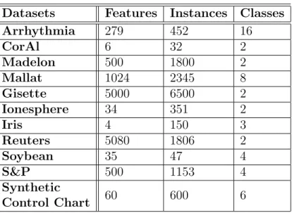
3.1.1 Principal Component Analysis and Singular Value Decomposition 30 3.1.2 Problem Formulation . . . 33 3.2 Related Work . . . 34 3.3 Weighted Scores . . . 37 3.4 Performance Evaluation . . . 39 3.4.1 Benchmark Datasets . . . 39 3.4.2 Peer Techniques . . . 43
3.4.3 Evaluation and Results . . . 44
3.4.3.1 Ranking Features and Minimizing the Residual . . . . 44
3.4.3.2 Discriminative Power of the Selected Features . . . . 47
3.4.3.3 Classification Improvement with Feature Elimination 49 3.5 Summary . . . 51
4 Feature Selection, Grouping and Engineering 53 4.1 Background and Preliminaries . . . 54
4.1.1 Problem Formulation . . . 56
4.2 Related Work . . . 56
4.3 FRG: Feature Ranking and Grouping . . . 58
4.3.1 Feature Weighting and Ranking . . . 59
4.3.2 Feature Grouping and Reduction . . . 61
4.4 Experimental Set Up and Results . . . 62
4.4.1 Benchmark Datasets . . . 62
4.4.2 Peer Techniques . . . 65
4.4.3 Evaluation and Results . . . 66
4.4.3.1 Ranking Features and Minimizing the Residual ∥A− CCA∥ξ . . . 66
4.4.3.2 Classification Improvement with Feature Selection and Grouping . . . 69
5 Transformation and Similarity Search 72
5.1 Background and Preliminaries . . . 73
5.1.1 Problem Formulation . . . 74
5.1.2 Number of Principal Component to Retain . . . 75
5.2 Related Work . . . 75
5.3 M2U Transformation . . . 77
5.3.1 M2U : Multivariate Time Series to a Univariate Time Series Transformation . . . 78
5.3.1.1 Finding the Weighted Scores(Variable Weights) . . . 80
5.3.1.2 Deriving the Univariate Signal . . . 82
5.3.2 Similarity Measure . . . 82
5.4 Performance Evaluation . . . 83
5.4.1 Benchmark Datasets . . . 83
5.4.2 Evaluation and Results . . . 84
5.5 Summary . . . 89
6 Trend and Value based Representation and Similarity Search 90 6.1 Background and Preliminaries . . . 91
6.2 Preliminaries . . . 92
6.3 Related Work . . . 93
6.4 Trend and Value Based Representation . . . 95
6.4.1 Similarity Measure . . . 99
6.5 Applying CTVR to Multivariate Time Series . . . 101
6.6 Performance Evaluation . . . 102
6.6.1 Datasets . . . 103
6.6.2 Evaluation and Results . . . 104
6.6.2.1 Impact of the number of segments on precision . . . . 104
6.6.2.2 Precision and Recall on the ARFSCMA dataset . . . 107
6.6.2.3 Execution time and precision as dimensionality in-creases on MTS . . . 107
6.7 Summary . . . 112
7 Conclusion and Future Work 113
7.1 Future Work . . . 115
1.1 Signal(s) representating a UTS(Left) and UTS(right) . . . 2
2.1 Time series representation techniques partly extracted from the tax-onomy in [81] . . . 15
3.1 Inosphere residual minimisation for 5 features . . . 46
3.2 Madelon residuals minimization for 20 features . . . 47
3.3 Arrethmia residual minimization for 5 features . . . 47
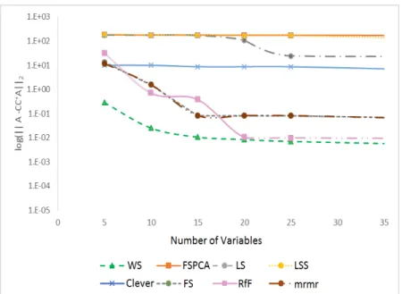
3.4 Reconstruction error ∥A−CCA∥ξ for selected features (5 to 35) on the Madelon dataset. . . 48
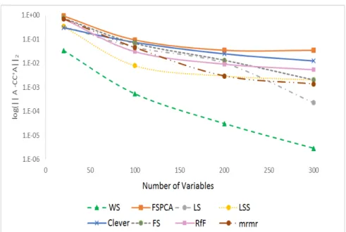
3.5 Reconstruction error ∥A−CCA∥ξ for selected features(20 to 300) on the S&P dataset. . . 49
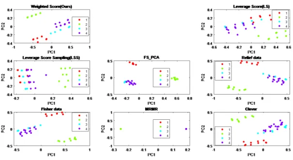
3.6 Synthetic Control data projection on the first two principal components 50 3.7 Soybean data projection on the first two principal components . . . . 50
3.8 Classification improvement with feature elimination . . . 51
4.1 Madelon residuals minimization for 20 features . . . 68
4.2 Inosphere residual minimisation for 5 features . . . 68
4.3 Reconstruction error ∥A−CCA∥ξ for selected features (5 to 35) on the Madelon dataset. . . 69
4.4 Classification accuracy of the nine techniques on a number of dataset. 70 5.1 Recall-Precision on AUSLAN . . . 84
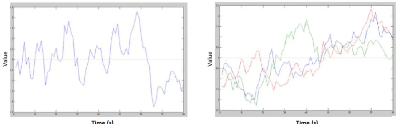
5.3 Left -Six images from the INRIA HID of three scenes taken at different points in time, found as closest matches. Right -Univariate signals for the six images after M2U transformation. Image names are color-coded
with their corresponding signal. . . 85
5.4 Runtime for each step in the proposed technique as the length of the time series increases (INRIA dataset) . . . 87
5.5 Runtime for each step in the proposed technique as the number of variables increases (INRIA dataset) . . . 87
5.6 Comparing the proposed technique runtime to that of Corr2 as the length of the time series varies . . . 88
5.7 Comparing the proposed technique runtime to that of Corr2 as the number of variables varies . . . 88
6.1 Steps in transforming UTS into symbolic strings using our proposed technique. . . 97
6.2 Proposed method illustration (ω = n). . . 98
6.3 Proposed method illustration (ω << n). . . 99
6.4 Precision as number of segments varies. . . 105
6.5 Identifying correlations while allocating more weight on value, trend or equally on both. . . 106
6.6 Precision/Recall on the ARFSCMA dataset for different techniques . 106 6.7 Run time for each step based on the number of variables . . . 108
6.8 Precision/Recall on AUSLAN(MTS) for different algorithms . . . 109
6.9 Accuracy on INRIA HID for different number of variables . . . 110
6.10 Runtime on INRIA HID as dimensionality increases . . . 111
6.11 Run Time for larger number of variables . . . 111
1.1 Vector representation of a UTS (a), Matrix representation of a MTS (b) 1
1.2 Table representations of a UTS(a) and MTS(b) . . . 1
3.1 Benchmark Datasets . . . 41
3.2 Iris & CorAl Features Ranking . . . 45
3.3 Ionosphere top 5 features selected by different techniques . . . 46
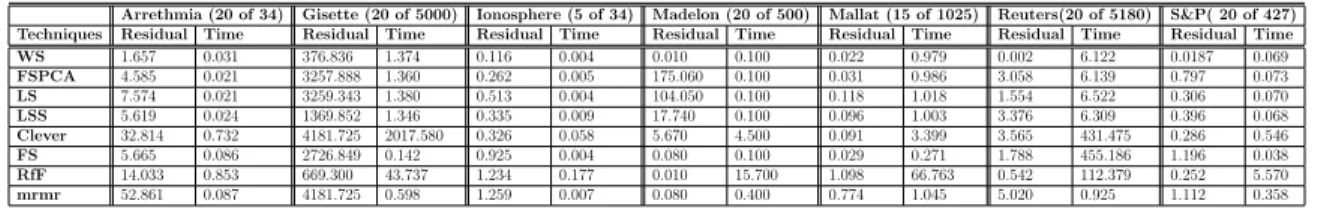
3.4 Minimizing the Residual ∥A−CCA∥ξ on Different Datasets Using Different Techniques . . . 46
3.5 Madelon Dataset 20 Most Representative Features Selected Using Dif-ferent Algorithms . . . 47
3.6 Percentage of variance explained for the first 6 principal components . 51 4.1 Benchmark Datasets . . . 64
4.2 Iris & CorAl Features Ranking . . . 67
4.3 Ionosphere top 5 features selected by different techniques . . . 67
4.4 Madelon dataset 20 Most representative features selected using differ-ent algorithms . . . 68
3.1 - Uncover the number k of PCs to retain . . . 39
3.2 - Weighted Scores (WS) . . . 40
4.1 - Feature Ranking and Grouping (FRG) . . . 63
5.1 - Find the number kmax of PCs to retain . . . 75
5.2 - M2U and Pairwise Correlation Search. . . 79
6.1 - Correlated Trend Value Representations(CTVR) . . . 96
6.2 - Efficient And Scalable Technique for MTS Similarity Search (ESTMSS) . . . 102
1.1
Time Series
A time series consists of observations recorded on discrete time points (discrete time series) or continuously through time (continuous time series) at regular time interval. Continuous time series can be discretized without much loss of information by using its inherently discrete type or techniques such as sampling or aggregation. Time series can be univariate or multivariate in nature.
⎛ ⎜⎜ ⎜ ⎝ −0.80 −0.29 −0.26 −0.45 ⎞ ⎟⎟ ⎟ ⎠ ⎛ ⎜⎜ ⎜ ⎝ −0.80 −0.51 −1.36 −0.29 −0.51 −1.43 −0.26 −0.70 −1.07 −0.45 −1.02 −0.73 ⎞ ⎟⎟ ⎟ ⎠ (a) (b)
Table 1.1: Vector representation of a UTS (a), Matrix representation of a MTS (b) t1 t2 t3 t4 Var1 -0.80 -0.29 -0.26 -0.45 (a) t1 t2 t3 t4 Var1 -0.80 -0.29 -0.26 -0.45 Var2 -0.51 -0.51 -0.70 -1.02 Var3 -1.36 -1.43 -1.07 -0.73 (b)
Figure 1.1: Signal(s) representating a UTS(Left) and UTS(right)
A univariate time series (UTS) T of length n pertains to one variable. It can be viewed as a point in an n dimensional space and expressed as: T= <x1, x2, . . . , xn>,
where xi is a real value in IR.
A multivariate time series (MTS) refers to time series that deal with recordings of values for more than one variable/attribute at regular interval of times. It can be viewed as a number of UTS. If m is the number of variables in a MTS A, we can write: A = (a11, . . . ..a1n), (a21, . . . a2n), . . . . (am1, . . . .amn).
Then, a MTS A that has n instances (of length n) and m variables can be repre-sented as an n ×m element matrix An×m, with n rows and m columns a follows:
An,m= ⎡⎢ ⎢⎢ ⎢⎢ ⎢⎢ ⎢⎢ ⎢⎣ a1,1 a1,2 ⋯ a1,m a2,1 a2,2 ⋯ a2,m ⋮ ⋮ ⋱ ⋮ an,1 an,2 ⋯ an,m ⎤⎥ ⎥⎥ ⎥⎥ ⎥⎥ ⎥⎥ ⎥⎦
Time series data represent a large fraction of the world’s supply of data [97] and, data generated in many applications can be transformed into time series without much loss of information [58, 56]. Hence, a growing number of applications in areas such as Finance, Neuroscience, health sciences require the ability to analyze and process such voluminous data. Unfortunately, when it comes to processing large time series datasets, the challenges already pertaining to time series in reduced settings (e.g. high dimensionality, redundancy or noise introduced through data collection
and the presence of dependencies between features) are of greater scale. On the other hand, most classical techniques are not adequately equipped to gracefully scale to larger datasets. Hence, pattern recognition on such data involves either tweaking the existing techniques or coming up with new ones that would adaptively process data in such environment.
Research in this field has been particularly active in recent years. While much has been achieved, the proposed techniques mostly focus on UTS and are not easily applicable to real life scenarios known to be better captured in multivariate abstrac-tions. Examples include the global economy, in which coexist a number of markets around the globe, trading a variety of financial products daily. Although one could be brought to think that, geographical locations or country local sovereignties and monetary regulation would make of the global financial markets a group of inde-pendent structures, it has been shown that asset prices often respond to the same global events [2]. In Neuroscience, the complexity of the human brain; its need for strong inter-connectivity and cohesion is better captured by also analyzing how voxels or regions of interest relate to one another than by merely analyzing voxels individually [85, 34, 52]. A multivariate analysis of time series data often considers the phenomena from an overall perspective, determines and leverages the intrinsic structure of the multivariate data, while providing a multi-layered analysis for better insights. In particular, research using correlation based techniques [48, 51,100, 103] such as the Canonical Correlation Analysis(CCA) or Principal Component Analysis (PCA) have shown that capturing and leveraging the information within MTS can be crucial in improving efficiency in many data mining areas such as similarity search, feature-subset selection, clustering, classification, hence the importance of develop-ing techniques that would work better for multivariate series with large number of variables.
1.1.1
Notation
This section provides the notation used in this thesis unless otherwise specified.
DU denotes the set of UTS.
An,m denotes a multivariate TS of n instances with m variables.
A, A = [aij] denotes a matrix representing the multivariate TS.
AT denotes the matrix transpose of A.
V is the right eigenvector matrix of sizem×m,Vk is the right eigenvector matrix
of size m×k.
S is the diagonal matrix of the singular values of A, Sk is the diagonal matrix
of the k largest singular values ofA.
ai,∗ denotes theith row of the matrix.
a∗,j denotes the jth column of the matrix.
ai,j denotes the element entry at the ith row and jth column of the matrix.
θ the explained variance in the data that are represented within k retained principal components
ρ is the Pearson correlation coefficient. ϵ is the user specified correlation threshold.
1.2
Thesis Objectives
The foundation of this research stems from two important aspects. First of which is the need to devise techniques that are better suited for today’s big data characteristics. And, the second aspect is the necessity to analyses and process data from highly unified frameworks such as an enterprise risk, the human brain, or a human organisms as multivariate concepts and rules rather than merely a concurrence of univariate ones. Highly unified frameworks present multilayed complexities that are better captured and conveyed through multivariate studies.
This research is focused on devising efficient and scalable techniques for time series data analysis and search, particularly for MTS, where we primarily relied on the PCA. The presented techniques retain the crucial underlying characteristics of the orig-inal MTS data, and leverage its structural properties for better interpretation. They size-ably reduce the time complexity and memory requirements for large datasets where storing the whole data in memory or relying on a large time complexity is not an option.
1.3
Thesis Contributions
This thesis presents a number of efficient and scalable techniques for MTS analysis and search. Our contributions, described as follows, particularly reside in the domains of dimensionality reduction and similarity search.
A feature subset selection technique, the Weighted Scores(WS) technique [48]: We first study the problem of uncovering the most relevant and discriminative features in a MTS. We analyze the MTS internal structure to find and leverage more information about the variables as they all do not equally contribute to the MTS. The technique relies on statistics drawn from the PCA to determine the weights of the variables with respect to the whole multivariate dataset and rank them accordingly. Subsequently selecting the set of most relevant features allows reducing the dimensionality while retaining the domain interpretability. The technique is unsupervised and sets a framework for improved efficiency in time series pattern recognition tasks such as classification, clustering or similarity search.
A feature subset selection and grouping technique, the FRG (Feature Ranking and Grouping technique) [49]: In some practical applications, feature subset selection alone may disregard important information when seeking for the most relevant and discriminative features in MTS. Those frameworks include MTS data exhibiting sparse feature vector structures, or Bio-informatics applications where dependent features are known to work better in groups than on their
own. In such cases combining feature selection to feature grouping yields better results [110]. We present an unsupervised feature selection and grouping tech-nique, namely FRG, that reduces noise, identifies relevant features, and groups correlated ones for increased efficiency and accuracy. The technique uses un-supervised learning through randomized PCA to determine influence and rank the features accordingly. Correlated features are then subsequently identified, grouped, and recombined into unique features to allow for a more efficient and scalable processing of high dimensional MTS.
A MTS reduction and representation technique, termed M2U(Multivariate to Univariate transformation) [50]: We present a PCA based MTS transformation technique that converts the MTS with large number of variables to a UTS prior to performing downstream pattern recognition tasks such as seeking correlations within a set of UTS. This technique is particularly important because, on one hand, the transformation takes into account the correlation between variables, in addition to decreasing redundancy and noise and, reducing the intrinsic high dimensionality. Other proposed univariate representations are often not able to retain the correlation between variables within each multivariate dataset. On the other hand, substantial recent research studied ways to improve efficiency for UTS pattern recognition tasks in general, and similarity search in particular [79,
88, 12, 71]. Our proposed representation will allow efficient UTS techniques to be easily extended to MTS data.
A UTS transformation and representation technique, TVR(Trend and Value Representation) [47]: We developed a UTS transformation and representation technique, TVR(Trend and Value Representation). This technique is obtained by extending the clipping technique [81,53,54] and incorporates the time series trend information, in addition to the value information in order to better capture the time series characteristics and providing greater accuracy.
The formulation of a similarity measure [47] based on a binary weighted dissim-ilarity measures for mixed types of variables measuring different objects: We
formulate of a weighted symbolic similarity measure measure based on a binary weighted dissimilarity measures for mixed types of variables measuring different objects. Using this similarity measure along with TVR in the pruning phase allows to substantially reduce the search space in large dataset frameworks.
An efficient and scalable technique for MTS Similarity Search: We proposed the use of the three techniques M2U [50], TVR [47] and the proposed symbolic correlation measure based on a binary weighted dissimilarity measure for mixed variables [47] in conjunction, to devise an efficient and scalable technique for MTS similarity search (ESTMSS). The technique improves computation time by at least an order of magnitude compared to other techniques, and affords a massive reduction in memory requirement while providing comparable accuracy and precision results in large scale frameworks.
These techniques contribute, from a general perspective, to the effort looking to address two sizable challenges that this area encounters: the high dimensionality of the data which makes it difficult to work with; and the scarcity of effective similarity search techniques for MTS.
1.4
Thesis Organization
The remainder of this dissertation is organized as follows. We review the background and related literature in Chapter 2. Chapter 3 presents the feature subset selection technique Weighted Scores (WS), followed by the feature subset selection and group-ing technique FRG in Chapter 4. The MTS reduction and representation technique M2U is introduced in Chapter 5. Chapter 6 discusses the UTS transformation and representation technique, TVR (Trend and Value Representation), followed by the formulation of a similarity measure based on a binary weighted dissimilarity mea-sures for mixed types of variables measuring different objects. Concluding remarks and future directions are presented in Chapter 7.
Work
Multivariate time series (MTS) data mining presents major challenges and, a fair amount of pre-processing is often required to improve the usability of the data for downstream pattern recognition tasks such as similarity search. The greatest chal-lenges encountered stem from the high dimensionality of the data, both in terms of length and number of variables, its volume and, the need to accurately assess simi-larities in time series. Core research activities in this area can essentially be classified into the following three areas: (1) time series data reduction and transformation, (2) time series similarity measures, and (3) time series indexing. Reductions and trans-formation techniques often look to uncover a reduced representation while retaining the important characteristics of the original data. Similarity measures help identify patterns and shapes. They assess how alike or different are time series based on given criteria. Time series indexing structures and techniques support efficient computation in terms of time and memory requirements. Our research goals and contributions fit in the first two core areas. In what follows we introduce the background and literature pertaining to those two core areas.
2.1
Time Series Data Reduction Techniques
Data reduction is widely recognized as an important preprocessing step for pattern recognition tasks; especially in large data frameworks. In the particular case of time
series, data reduction can often be seamless. This is due to the fact that time series data inherently presents a structure such that, it generally exhibits some amount of redundancy. A given point may influence many nearby observations though auto-correlation, and two successive data points can often be within a predictable range, hence presents the possibility to seamlessly reduce the data.
While many data reduction and representation strategies have been proposed, the techniques must be carefully chosen to ensure their suitability for the data at hand and, for the intended downstream tasks. Doing so, ensures the effectiveness of the overall mining technique. Time series data reduction techniques can be generally categorized in three core areas: data compression, numerosity reduction, and dimen-sionality reduction; although dimendimen-sionality reduction and numerosity reduction may be considered as forms of data compression.
Data compression techniques primarily provide a strategy to minimize the amount of data (or number of bits) needed to be stored or transmitted. Compressions can be qualified as either lossless or lossy. Lossless compressions generally rely on data redundancies to reduce the data without losing information, and hence, allow for a recovery of the full information when uncompressed. Lossy compressions on the other hand, rely on strategies that reduce the data by omitting nonessential information according to human perception for instance. They ideally present an acceptable level of information loss with respect to the gain in other aspects such as memory space or time complexity.
Numerosity reduction techniques use parametric and non-parametric models such as sampling, histograms or clustering to estimate the original data and replace it by smaller forms of representation. For instance, in the case of the parametric model, once the data has been estimated using the parametric model, storing the parameter rather the original data is common practice.
Dimensionality reduction techniques seek to uncover or devise a rich reduced set of features that retain crucial underlying structure from the original data. More formally stated: given a set of n pointsX = {n∈IRd}in a high dimensional Euclidien space, we look to describe X in fewer dimensions k << n, d without distorting the Euclidien distance between any two points by much (by less than a well defined small
ϵ).
Otherwise expressed, define a function f such that∀xi, xj ∈X
∣∣f(xi) −f(xj)∣∣2≈ ∣∣xi−xj∣∣2. (2.1)
Dimensionality reduction techniques include feature extraction, feature selection or feature re-engineering techniques. The state or art techniques are often based on one or a combination of some of four widely used techniques: (1)Fourier transform, or a derivative of the Fourier transform (2) the Wavelet transform, (3)the Singular Value Decomposition, and the (4)Random projection technique. Depending on the type of data at hand, some techniques may be more suitable to consider than others. In what follow, we introduce those four widely used techniques but first define some notions that they shared.
Definition 2.1. (Orthogonal Transformation) Given two vectorsu⃗and ⃗v, an orthog-onal transformation T: V -> V of u⃗ and ⃗v to T(u⃗) and T(v⃗) respectively is a linear transformation which preserves symmetric inner product. In particular, it preserves the length of the vectors and the angle between the vectors.
Definition 2.2. (Orthonormality) - Given two vectors u⃗ and ⃗v in an inner product space ( a vector space that has an additional structure called inner product, generaliz-ing the dot product) ,u⃗and v⃗are said to be orthonormal if they are both unit vectors (their lengths are each equal to 1) and are orthogonal (the angle between them is 90). An orthonormal set of vectors is comprised of vectors that are all pairwise orthogonal and of unit length.
The Fourier transform [23], originated from results first introduced by Jean Baptist Joseph Fourier in 1807 stating the feasibility of expressing any piecewise con-tinuous periodic function with period T, as the sum of a (possibly infinite) set of oscillating functions, based on the sines and cosines and, whose frequencies are mul-tiple of the angular frequency ω0 = 2Tπ. Those results were further extended to any
a sum of their Fourier series (or complex exponentials) and expressed as:
f(t) = a0
2 +∑
∞
k=1 (akcos 2kπtT + bksin 2kπtT ) where:
a0= T2 ∫ T 2 −T 2 f(t)dt, ak=T2 ∫ T 2 −T 2 f(t)cos2kπtT dt, k = 1, 2, 3, . . . bk= T2 ∫ T 2 −T 2 f(t)sin2kπtT dt, k = 1, 2, 3, . . .
The Fourier transform decomposes and analyses a function of time into its fre-quency domain, rather than its time domain. For data that is discrete in nature such as time series, the Discrete Fourier Transform (DFT) is more appropriate. This technique is based on orthogonal transforms where the coefficients are uncovered by carrying out an inner product between the input signal and a set of orthonormal basis functions. It is often preferred when the data is periodic due to the periodic nature of the functions used to approximate the original data. The original time series data is transformed into frequency components sorted in decreasing order of importance. As the first few components often carry most of its so called energy, ignoring the remaining components known as negligible is appropriate. Once the dimensionality is reduced, the Fourier domain affords a framework where data processing is more efficient. An approximation of the original features can be reconstructed by using the available components.
The time complexity of the fast Fourier transform is such as for a time series of length n, computing the k first component takes Min (O(nlogn), O(kn)). Clearly, although acceptable some other techniques such as the Discrete Wavelet transform (DWT) reviewed next, present a better time complexity.
The Wavelet transform is an orthogonal transform and a derivative of the Fourier transform. The first wavelet transform known as Haar wavelet [28] was intro-duced by Alfred Haar in 1909 although wavelets were not yet defined as such until Jean Morelet coined the concept in 1981. Similarly to the way the Fourier transform relies on thesinandcosfunctions as its basis functions to decompose other functions,
the wavelet transform leverageswavelets as its basis functions. WithΨ(t) ∈L2(R)set
as the mother wavelet, it may be transformed and dilated through critical sampling. The wavelet transform may be expressed as:
W f(a, b) = ∫−∞∞ f(t)√1
a Ψ
∗ (t−b
a )dt ∣b∈R,a∈R+
where b is the translating parameter, indicating the corresponding region, a is the scaling parameter greater than zero because negative scaling is undefined.
In this framework as well, the discrete wavelet transform (DWT) is more appro-priate for data with discrete time points such as time series and an inner product between the input signal and a set of orthonormal basis functions allow to uncover the coefficients.
The family of DWT present a key advantage over the DFT in that they are multi-resolution transforms, hence allow to efficiently operate in both the spectral and time domains. Indeed, although a particular case of the Fourier transform known as the Short-time Fourier transform (STFT) may provide both time and frequency information, the resolution in frequency may be limited by the fixed size sliding window used to uncover its spectrogram. The Wavelet transform affords a framework that not only enables the intrinsic analysis of the time series’ frequency but also provides other important insights such as the scale of the time series or time at which a specific observation occurred.
It is also possible to reconstruct an approximation to the original time series by using the coefficients that result from the DWT. The scale of the transformation, or amount of details in the signal, plays an important role in the reconstruction process. Coarser resolution coefficients pertain to small scales and allow for better data reconstruction than the higher resolution coefficients that refer to larger scales. The time complexity of the DWT for a signal of length n is O(n) (wavelet transforms without compact support may however require O(n2)).
The Singular Value Decomposition (SVD) is an orthogonal linear transfor-mations in which one assumes all basis vectors to form an orthonormal matrix. It projects the original dataset in a new coordinate system where the directions are pair-wise orthonormal. It has been used in many applications primarily for the following key advantages:
reduces redundancies and noise introduced during the data collection process. reduces the number of variables while retaining the variability in the data. identifies relationships and interactions between variables.
identifies hidden patterns and classify them according to the amount of infor-mation stored in the data.
The SVD may be used as an important step in many other powerful dimensional-ity reduction techniques such as Principal Component Analysis(PCA) [48], Canonical Correlation Analysis(CCA) [9] or Independant Component Analysis(ICA) [33] among others. The basis vectors of the SVD are however data dependent which presents both advantages and disadvantages. Among the disadvantages is the need to store the basis vectors in addition to the new data points in order to be able to reconstruct the origi-nal data [114]. Although this technique currently provides the best approximation to an original matrix, computing the SVD of a large matrix of n instances and m vari-abes can be expensive with a time complexity of O(min(n2m,m2n)) if randomization
techniques are not used.
TheRandom Projections technique, unlike the DFT, DWT, SVD, is not based on orthogonal transformations, but rather on a projection of time series randomly to a lower dimensional space. It is fundamentally based on the Johnson-Lindenstrauss lemma proposed in 1984 [40] and stated as:
Lemma 2.1. (Johnson-Lindenstrauss Lemma)
For any 0<ϵ<1 and any interger n let k be a possitive interger such that
k≥ 24
3ϵ2−2ϵ3 logn (2.2)
then for any set A of n points ∈IRd
there exists a map f ∶IRd→IRk such that for all xi, xj ∈A
The lemma conveys that, given a set of points in a high-dimensional space, they can be projected and embedded into a lower dimensional subspace, such that distances between the points are nearly preserved.
For random projections, the lower dimensional subspace is randomly chosen based on some distribution and, we can seek to have a probabilistic guaranty that the distance between two time series in the higher dimensional space will have some sort of correspondence with the distance between the same two time series in the lower dimensional space. Considering a matrix An×m the original data with m variables
and n observations, then Ak×m =Rk×nAn×m is the random projection of An×m onto a
lower k-dimensional subspace. This technique is carried out by using a random matrix whose rows have unit lengthsRk×nand projecting the original n-dimensional data onto
a k-dimensional (k << n) subspace. The time complexity of such a transformation is O(nkm). Unlike DFT, DWT and SVD, the random projection method does not allow to reconstruct the original data. This technique is known to be efficient for frameworks with relatively small numbers of very long time series due to the fact that, the data size k resulting from the reduction does not depend on the time series instances but on the number of time series [114]. It is however known to be less effective than PCA for severe dimensionality reduction [24].
In this thesis work, since our intent is to substantially reduce the dimensionality without impacting time and accuracy, we essentially use either the standard SVD, or randomized versions of the SVD [30, 17] in our computation of the PCA (discussed in Chapter 3), which allows to achieve those objectives as we will see in Chapters 3, 4, 5 and 6.
Dimensionality reduction techniques often provide time series representations strate-gies that afford a framework where large scale data becomes more manageable. Such representation techniques can primarily be grouped into four classes [81], as illustrated in Fig.2.1. The classes are labeled according to the nature of transformation applied to the data: model based, data adaptive based, non-data adaptive, and data dictated. Model based time series representation techniques often use the parameters driving the model to represent the time series. In this case, comparing two times series may be carried out by checking whether they have the same set of parameters driving the
Figure 2.1: Time series representation techniques partly extracted from the taxonomy in [81]
model. Non-data adaptive techniques rely on the same set of transformation parame-ters for all types of data, regardless of their specificities or of the differences between their respective features. Most non-data adaptive techniques can be transformed to data adaptive techniques by adding a data sensitive selection step [21]. Data adaptive representation techniques assume that, during the transformation process, parameters of the transformation such as the compression ratio of the data are influenced by the internal structure of the data. The SVD for instance is a data adaptive representation technique that works particularly well for data where linear dependencies exist.Data dictated representation techniques rely on a compression ratio that is data dictated.
For instance, in the particular case of of the clipping technique, the time series record-ings are transformed into bits, where each bit value is indicative of the corresponding point’s position with respect to the average. Clipped data [81,53,54], consisting of a sequence of symbolic bits has the advantage of being directly comparable to the raw time series data.
Our proposed Trend and Value Representation(TVR) technique incorporates tech-niques from three different classes: a non-data adaptive technique(Piecewise Aggre-gation Approximation(PAA)), a data adaptive technique (Symbolic AggreAggre-gation Ap-proximation(SAX)) and a data dictated technique (clipping); although clipping can be considered a particular case of the SAX representation [81]. Hence, this allowed to leverage advantages from all three classes of techniques as we will see in Chapter 6.
2.2
Multivariate Time Series Similarity Search
Re-lated Literature
Similarity search can either be regarded as a stand-alone task or as a crucial step in many data mining tasks such as indexing, classification, clustering or anomaly detection [79].
An important step in a similarity search process is devising a similarity measure to assess how alike or different are time series based on given criteria. When seeking similarities between time series, one can consider many aspects, among which simi-larity in time, in shape or in change. The simisimi-larity in time otherwise implies how correlated are time series. The similarity in shape seeks for the likeness in patterns of change, irrespective of the time points. The similarity in change considers the likeness in auto-correlation structure.
The choice of the similarity measure often depends on a few aspects among which the type of data at hand, the feature(s) that we look to compare, and the type of application we are dealing with.
paradigms that guide them: shape based measures, edit based measures, feature based measures, and structure based measures. Shape based measures seek to compare the general shape of two time series. Edit based measures tend to first transform the time series to a alternate representation then to assess the minimum number of operations required for the transform to occur. Feature based measures investigate and extract important features from original time series then, subsequently compare the extracted features using a distance measure. The aim of the structure based measures is a bit similar to that of the shape based measures, with respect to the fact that they look to compare the time series from an overall perspective. The structure based measures often seek to find high level structures in the data, which will allow for a comparison in an overall perspective. The structure based measures are further considered compression based when they analyses how well the time series can be compressed together; higher compression ratios make better similarity measures. On the other hand they are considered model based when the strategy is to fit a number of time series to a model, then assess the similarity by comparing the model’s parameters.
The work in this thesis investigated similarities in time and shapes, while linear dependency was an important factor. We essentially used Pearson correlation as the measure to assess similarity between two time series.
Research in time series similarity search has attracted the attention of many re-searchers, resulting in much progress in recent years, particularly for UTS. We can divide the research activities and results since the 90s to three periods.
The early years, from 1994 to 2003 represent a period which described concepts along with the technique strategy and provided implementation guidelines. The pro-posed techniques in this time period mainly focused on UTS and smaller dataset sizes.
During 2003 to 2008, two tendencies were more pronounced. A first one where the research investigated techniques proposed at the time and looked to improve them, or devise more efficient strategies. A second tendency reflected a moment where the research community had started to understand the importance of devising techniques for MTS. Indeed, it became clear that many situations are in fact only part
of complex occurrences that involve many interrelated aspects. Such situations are better represented by multivariate concepts and rules, than by compounded isolated effects from univariate ones. A MTS data analysis affords a multi-layered analysis, uncovers interactions between variables, and provides an overarching view of the internal structure for better insights. Although there were serious attempts at the time and good progress was achieved, the literature often focused on MTS with low number of variables.
Since 2008, several solution techniques were proposed to improve similarity search and related applications such as clustering or classification. We can note three par-ticular shifts in the current literature.
The first shift represents a tendency of moving away from theoretical “Toy prob-lems to realistic deployments” [35] to address the real world problems. For instance, a clear effort to develop techniques that would process time series data as received, with its imperfections (uncleansed data, different length series, etc.) [35,36, 92].
The other two shifts are found in the literature looking to address today’s big data challenges. Those challenges essentially stem from its magnified characteristics in terms of volume, variety, increased need for velocity, veracity and value.
Where one focuses on processing scalable and efficient search in large size data, the second one focuses on scalable and efficient search in MTS with larger numbers of variables and dimensions. The latter is the focus of this thesis work.
The research trend focused on efficient and scalable search in large size data is mostly directed to UTS (search across large numbers of UTS, millions to trillions of them) and heavily relies on indexing. In particular, we note the work of Shieh and Keogh [87] who proposed a technique for indexing and mining terabyte sized time series, or Camerra et al. [12], for indexing and mining a billion of time series in later work. In 2012, a study by Rakthanmanon et al. [79] proposed a method for searching and mining trillions of time series subsequences by combining 4 techniques, allowing for early abandoning and using Dynamic Time Warping. ”The difficulty of scaling search to large datasets largely explains why most academic work on time series data mining has plateaued at considering a few millions of time series objects, while much of industry and science sits on billions of time series objects waiting to be
explored” [79]. While much has been achieved with the techniques in this trend, they mostly focus on indexing techniques and on UTS. More work is required to develop techniques that would work better for MTS.
The second research trend focuses on efficient and scalable search for MTS with a large number of variables (and often higher number of instances) that generally follows one of three approaches. In the first approach, each variable within the MTS is considered independently as a time series [22], and often analyzed separately by using univariate techniques. While being easier to process, this approach often re-quires much more computation time. The second approach consists of stacking all data contained within all variables as a lengthy UTS [46], to be analyzed as such, using univariate techniques. Like the first approach, this strategy often overlooks the relationships that exist among the variables and cannot efficiently process a relatively large number of variables. The third approach, considers the MTS as a whole and transforms it into a lower dimensional representation that still captures its main char-acteristics, and the hidden relationships among variables, while rendering the data more manageable [86, 103, 82]. Although this approach presents more complexity, it provides more accurate results for similarity search. Techniques of this third ap-proach can often be classified into two groups; those that deal with streaming time series data, and the rest. In the following subsections we will review these techniques.
2.2.1
Multivariate Time Series Similarity Search Techniques
for Data in Motion (Streaming Data)
The first group of techniques, proposed to identify patterns in streaming time series, which is continuous, unbounded, and a timely ordered sequence of data elements generated and/or collected (at a rapid rate). These series may include multiple mea-surements at each time point hence, they can be looked at as MTS.
A notable work in this area is an approach for discovering correlations and hidden variables in multiple streaming time series, introduced through SPIRIT((Streaming Pattern dIscoveRy in multIple Timeseries) by Papadimitriou et al. in [75]. The dis-covered information would be used to summarize the entire trend in the set of streams
and, allow for fast forecasting and outliers detection. This technique is based on PCA and satisfies some important goals of online streaming algorithms such as automatic detection of patterns, adapting to the changes in real-time, scaling up linearly with the number of time series and, suitability for distributed environments.
In a practical application, Sayal et al. [84] introduced a method for extracting time correlations among multiple stream time series. The proposed method expresses time correlations as reusable correlation rules and textual representations conveying observed dependencies or relationships among stream time series. For instance, the observation that a change in the values of one set of time-series data streams initiates a chain effect that causes the change in the values of another set of time-series data streams. For example, if the value of an attribute A increases more than 5%, then the value of the other attribute B is expected to decrease by more than 10% within two days. More precisely, in an IT operational environment, a server performance has a time-delayed impact on database performance that can be quantified according to proposed rules. The proposed method consists of three main steps. In the first step, the original time series data was summarized by aggregation at different time granularities. In the second step, the change points upon which the comparisons were based were detected using CUSUM in order to reduce the search space and convert continuous data stream into discrete data stream. In the third step, the correlation rules were generated. The proposed method used sampling techniques to determine a few candidates to work with in order to speed up the search.
Wang et al. [99] proposed a technique for similarity search and discovery of pat-terns in time series. Using a vector quantization technique for dimension reduction and a symbolic representation of time series, they apply a string matching technique, LCSS (longest Common subsequence), to compare time series of different lengths. The authors address the case of a nearest neighbour of the input query with a thresh-old given for the distance measure. The proposed solution partitions each sequence into equivalent length segments and uses vector quantization to represent each seg-ment into a codebook. The similarity measure is then carried out using an extended version of the LCSS that will allow to compare sequences of different lengths.
correlation analysis in stream time series. Using binary sequences to dynamically represent streaming time series, a similarity search and clustering operation is ran on incoming streams. The article focused on fast correlation analysis in a large number of stream time series and proposed a technique called HBR (Hierarchical Boolean Representation). The technique processes a large number of incoming stream series, transform them into boolean series, before to check their pairwise correlation values against given correlation thresholds. A candidate set is then identified as containing all series for which their boolean versions are correlated above the given thresholds. An extension of the Pearson similarity measure is subsequently used to compute the correlation value between original time series selected as part of the candidate set.
The problem of exploring and identifying correlations among multidimensional arrays of data stream (particularly between two such arrays in environments with limited resources) was explored by Wang et al. [100]. For this, they propose to use an improved version of the standard canonical correlation analysis technique (CCA). When used in its standard form CCA (or NaiveCCA) does not perform well for multidimensional time series. This technique , termed ApproxCCA [100] uses an incremental computation paradigm and low rank approximation technique based on unequal probability sampling to reduce the dimensionality of the product matrix (composed by the sample covariance matrix and sample variance matrix). The pro-posed changes were mainly carried out in two steps: an incremental computation performed on the variance and covariance matrices, and a low-rank approximation conducted on the product matrix to obtain the canonical eigenvalue and the canonical correlation eigenvector.
In recent years we witness more research effort looking to apply real world sit-uations [36, 80] where data can be efficiently processed with its imperfection (e.g. uncleansed). An example of such trends is the work in [36] by Hu et al. which is in-tended to be robust for environments with irrelevant and missing data scenarios. The technique is based on the general techniques of weighted voting and Bayesian classifi-cation and, extends the techniques of dictionary-based classificlassifi-cation. More precisely, a framework to classify multi-dimensional time series by weighting each classifier’s track record is proposed. The classifier’s track record weights are themselves based
on each stream’s previous track record on the class it is predicting at the moment, but also on the distance from the unlabeled object.
Raptis et al. [80] presented a real-time wireframe for skeletal motion classification. The key components of this technique include three aspects: an angular representation of the skeleton, to render recognition more robustness for noisy input, a cascaded correlation-based classifier for MTS data with a distance metric based on dynamic time warping to evaluate the difference in motion between an acquired gesture and, an oracle for the matching gesture. While the first two key components can be re-used for other skeletal motion classification scenarios, the oracle for the matching gesture is specifically tailored for a known canonical time based musical beat. The technique provides a framework that serves to guide individuals during exercise sessions (in this case dance instead of rehabilitation).
While some progress has been noted in the area of streaming MTS analysis and search, it is still in its infancy and more advanced techniques are needed to seamlessly and adaptively cater to streaming data in large data frameworks, regardless of its arrival rate. In this thesis work, we developed efficient and scalable techniques for MTS data at rest that we plan to extend to streaming data frameworks in our future work.
2.2.2
Multivariate Time Series Similarity Search Techniques
for Data at Rest
The second group of techniques concerns MTS similarity search for data at rest. While techniques in this group are today increasingly investigating big data challenges pertaining to MTS with large number of variables and instances, early techniques, investigated multivariate time series with fairly small number of variables. They often relied on indexing techniques. Those early techniques included the work of Vlachos et al. [98], investigating similarity search in the trajectories of moving objects in two to three dimensional spaces with different orientations. The technique used an indexing scheme that leverages the hierarchical tree of a clustering algorithm for nearest neighbor queries. The technique afforded among other things, a time
series normalization strategy, a mapping of trajectories to space that would be robust against rotations and translation scaling, an elimination of the noise that results from vertical shifting by mapping the spacial coordinates of the trajectories to sequences of arcs and angles pairs prior to normalization. It also accommodated assessing the similarity between variable lengths time series data.
In a similar framework, Chen et al. [14] also studied MTS similarity in relation with moving object trajectories. Data from such frameworks is known to be carrying much noise, hence this technique like many others investigated ways to devise a technique that would be robust against noisy data. An extension to the Edit or Levenshtein distance was introduced as Edit Distance on Real sequence (EDR). It allowed to assess the dissimilarity between two objects by counting the minimum number of edit operations required to transform one object into the other, while handling local time shifts and assigning penalties to the unmatched parts. The distance measure was combined with different implementation methods of three pruning techniques, known as mean Q-gram techniques to improve the retrieval process.
The other strategy within this group of techniques is attempting to reduce di-mensionality and transform the MTS prior to measuring the similarity for relatively larger number of variables. This latter strategy seems more suited for multivariate time series with large number of variables due to the fact that, when careful selected, the dimension reduction techniques often allow for more efficient data processing. In this framework, Yang et al. [103], proposed a similarity measure for MTS, based on PCA, called Eros (Extended Forbenius Norm). The authors propose to represent two MTS as two matrices (e.g. A and B), whose PCA are computed to uncover their respective eigenvalues and eigenvectors. The eigenvalues and eigenvectors are then subsequently used to uncover the dataset weight vector w and measure the similarity between the two matrices. Provided with the two original matrices and the dataset weight vector w, the technique assesses the similarity between the two datasets by computing Eros(A,B,w)=∑ni=1wi∣ <ai, bi> ∣, where <ai, bi>is the inner product of ai
and bi. This proposed similarity measure does not satisfy the triangle inequality, but
can be provided with an upper and lower bounding by using the weighted Euclidean distance. In combination with Eros, a search based K nearest neighbors (KNN) for
MTS is proposed. Experimentally, the proposed solution outperforms the Euclidean distance(ED), Weighted Sum SVD (WSSVD), Dynamic Time Warping (DTW), and the PCA similarity factor (SPCA) in terms of precision and recall. It also presents a better time complexity than the Euclidian distance and DTW.
Yang et al. further investigated the idea in [104] by exploring how the stationarity of the time series might impact the proposed technique. The time series were first rendered stationary before processing. A time series is considered stationary if its correlation is stable, i.e. if its statistical properties such as the mean and the cor-relation coefficients, do not change over time. Applying Eros on brain stimili time series rendered stationary showed a performance improvement in precision and recall of over 24%.
Karamitopoulos et al. [51] proposed a MTS similarity search technique based on reducing the MTS data set size and dimensionality using a principal component analysis (PCA) signature prior to measuring similarity. The idea explored in the paper is the recognition that if two MTS are similar, their PCA representations will be similar in some way as well. An interesting aspect of this similarity search technique is that it does not directly rely on applying each time a intensive computation of the PCA to query frequently arriving object in order to match them to the most similar objects in a database or classify them into predetermined classes. Rather, the resource intensive computations of the PCA are conducted only once to build up a database of PCA signatures, which will be subsequently used to allow the quicker identification of a query objects most similar correspondent in the database.
Tanaka et al. [94] devised a technique for finding motifs in MTS. This technique, like many in this group, also relies on the recognition that if two multivariate time series are similar, their PCA representations will be similar in some way [51,4]. The technique first relies on dimensionality reduction and transforms the MTS to a UTS by applying a standard PCA. It retains the first principal component to be used in the subsequent steps. The dimensionality reduction is followed by a transformation of the data to a sequence of symbols using SAX(Symbolic Aggregate Approximation) [67] an extension of the PAA (Piecewise aggregate approximation) [107, 57] technique. The technique subsequently looks to find motifs using the MDL (Minimum Description
Length) principle on all dimensions of the MTS. While, this technique provides good results for relatively low number of variables, and cases where the first principal component carries a large amount of the explained variance, computing the standard PCA algorithm on a large matrix normally requires O(min (n2m, m2n)), which can
be prohibitively expensive in large dataset environments. Techniques transforming the multivariate time series to the univariate domain often yields better results as they tend to retain more characteristics from the original data [86, 82].
Banko et al. [4] proposed to use the correlation based dynamic time warping (CB-DTW) technique to find correlations between MTS for applications in MTS recogni-tion. This technique goes through three steps to assess the similarity between MTS. In the first and second steps, the time series of the given database and the query time series are segmented respectively; in the third step the distance between the two is assessed. The segmentation strategy is the same for both the query and the time series contained in the database. A key aspect in this segmentation process is the need for homogeneous segments, hence correlation was used for that purpose. The segments are obtained by bottom-up segmentation, where every element of the whole UTS within a given MTS is handled as a segment and the costs of the ad-jacent segments are calculated (using special, PCA related cost). Subsequently two segments with the minimum cost are to be merged. This being a top down strategy, The merging and cost calculation of adjacent segments continues until some set goal is reached. After the MTS are segmented, the third step consists of assessing the DTW dissimilarity between the query and the time series from the database. For that purpose the PCA similarity factor (SPCA) is uncovered on each segment to feed the dynamic time warping (DTW) local dissimilarity function. In combing DTW and PCA based similarity measures, the technique preserves the internal correlation that exist between variables, and allows for advantages such as a robustness against phase shifts of the time axis, or accommodating differences in sampling rates. The tech-nique outperformed peer techtech-niques on the 2004 competition database of signature verification and the AUSLAN datasets.
In applications to classifications, Esmael et al. [22] proposes a technique for MTS classification. The technique extends the Symbolic Aggregate Approximation (SAX)
technique [67] using three new string symbols (U, D and S) to represent the trend of the time series (UP, Down, Straight). First each variable within the multivariate time series is divided into a sequence of smaller segments by sliding a window incrementally across the time series. Then the algorithm transforms the numerical values of each variable in the given time series into a sequence of ⟨value, trend ⟩ pairs. While a good level of precision can be expected from this technique because the quantization happens directly on the data, it will not easily scale to large multivariate dataset environments, where the number of variables are expected to be sizably larger.
Also in a clustering/classification frameworks, Spiegel et al. [92] proposed an ap-proach that can be generalized for contextual pattern detection in multivariate sensor data. The technique consisting of three steps: feature extraction based on important time series characteristics to devise learning models, uncovering internally homoge-neous time intervals and change points through segmentation, and finally clustering and/or classifying time series segments into the sub-population to which they belong to, based on contextual similarity. The segmentation procedure relies on a PCA based segmentation technique derived from a time-varying multivariate data segmentation method. The latter is known to be robust for signal processing and complex drive ma-neuvers that consist of multiple consecutive time series segments. Examples of such maneuvers include for instance ”stop and go at traffic lights or overland drives” [92]. In this trend of research as well, much progress has occurred in recent years. However there is still a need to improve on many aspects of the current available techniques. As we will see, in Chapters 3, 4, 5, and 6, our introduced techniques provide improvements on precisions and recall, memory space usage and processing time when compared to peer techniques.
2.3
Summary
Multivariate Time series analysis has grown in importance, relevance and popularity in recent years. Traditional methods for uncovering meaningful patterns are no longer suitable in today’s high dimensional data processing frameworks. In this Chapter, we
introduced the background and literature pertaining to data reduction and similarity search in MTS. Although good progress has been achieved, more work is required to improve on many aspects of the current available techniques. For instance, much of the current literature for similarity search is still focused on fairly low size multivariate problems with less than 150 variables. In addition, even finding suitable ways to reduce and represent time series in the preprocessing stage is still an open problem.
We however believe that better results for MTS analysis and search in large data frameworks can be achieved by combining some important aspects among which the following three:
understanding that high performance data driven discovery or unsupervised learning in MTS is becoming a necessity in large data frameworks.
leveraging powerful tools and techniques such as the Principal Component Anal-ysis(PCA), Randomized Matrix Theory aided by a heightened computational power,
adopting a multidisciplinary approaches to allow for a richer and broader re-search frameworks.
Our contributions in Chapters 3, 4, 5 and 6 follow those lines of thoughts. In the next Chapter, we introduce an efficient dimensionality reduction, and more precisely feature selection technique using PCA and based on unsupervised learning.
In this chapter, we introduce the Weighted Scores(WS) technique, an unsupervised learning technique to identify the top-k discriminative features for multivariate time series(MTS).
The Weighted Scores technique uses statistics drawn from the Principal Compo-nent Analysis (PCA) of the input data to leverage the relative importance of the principal components along with the coefficients within the principal directions of the data to uncover the ranking of the features. In what follows, we review the back-ground and preliminaries in Section 3.1, discuss the related work in Section 3.2, and introduce the technique in Section 3.3. Section 3.4 presents the performance eval-uation. A summary, our concluding remarks and future directions are presented in Section 3.5.
3.1
Background and Preliminaries
Innovation and advances in technology have led to the growth of data at a phenomenal rate. Paradoxically, the existing MTS data reduction, analysis and mining techniques do not scale well to its current challenges. Among those challenges, the presence of noise and redundancies in high dimensional data for many practical applications makes it difficult to uncover important patterns. Hence, most pattern recognition tasks rely on dimensionality reduction through feature extraction or feature selection as crucial preprocessing steps, for reasons of efficiency and interpretability, for a better understanding of the underlying processes that generated the data, but also to build
a framework that allows downstream pattern recognition tasks such as classification, clustering or similarity search to perform more efficiently.
While feature extraction and selection both ultimately allow to use a reduced set of features to achieve higher or similar accuracy results as using all features, they differ in terms of strategies. On one hand, feature extraction relies on transforming existing features/variables into a lower dimensional space, and creating a new and reduced number of features from original features. The new features are conceived so to have the largest possible variance, since the percentage of explained variance retained for the new variables indicates the amount of information retained within the reduced data. The larger the variance retained, the lower will be distortion at reconstruction. Feature extraction techniques often can uncover the new embedding space in linear time, making them preferred in terms of computational complexity. Unfortunately, the transformation process in feature extraction methodologies can render the newly extracted features difficult to interpret.
On the other hand feature selection (also known as variable or attribute subset selection), identifies a subset of most relevant features from the original set to be used for subsequent processes. The difference in reduction strategies makes feature selection preferred as a dimensionality reduction method for practitioners in cases where the interpretability of the reduced subset needs to be maintained with respect to the originally acquired features, or when there are far more features than samples [27]. The feature selection process is however a combinatorial optimization problem, which is NP Hard [72,15]. To uncover the needed subset in reasonable time, most techniques in this area rely on heuristics. In our case, we rather rely on matrix decomposition. We present a simple yet effective and scalable unsupervised feature selection technique based on statistics drawn from the Principal Component Analysis (PCA) [41] of the input data. While this technique leverages the desired properties of the PCA, it retains the results interpretability of the results by combining the advantages of feature extraction and selection techniques.
An important aspect of this technique is the recognition that not only the co-efficient within the principal directions are crucial in identifying the importance of variables, as seen in major related work [41, 109, 18, 90] but also more importantly
each principal component should be weighted with its relevance during assessment of the variable’s weight.
Our empirical evaluation in a large number of application domains using numerous benchmark datasets indicate our proposed technique improved performance in terms of accuracy, speed, and scalability.
3.1.1
Principal Component Analysis and Singular Value
De-composition
In this section we review the PCA and SVD techniques which form the basis for our proposed techniques in Chapters 3, 4 and 5.
The PCA and SVD are orthogonal linear transformations and matrix decompo-sition techniques that project the original dataset in a new coordinate system where the directions are pairwise orthonormal. A main advantage of these techniques in our work is that they guaranty the uncovering of an optimal reduced embedding with minimal approximation error, and hence retains the crucial underlying structure of the original data. The PCA and SVD are amongst the most efficiently computable techniques and powerful tool of choice for reduction of high dimensional data. Be-sides, these two techniques decrease redundancy and noise, highlight relationships between the variables, and reveal patterns by compressing the data. They help iden-tify similarities and dissimilarities as well. Using these two techniques on raw MTS data often requires some preprocessing such as mean-centering and scaling to adjust values measured on different scales to a relatively common scale, since PCA is a vari-ance maximizing technique. In addition, some conditions [93] on the raw input data have to be met for the results from the PCA/SVD to be numerically stable and valid. These conditions are primarily as follows:
The relationships between variables must be linear.
There should be ”adequate” redundancies amongst the variables through cor-relation to allow summarization of the variables into a rich, reduced set of components.
![Figure 2.1: Time series representation techniques partly extracted from the taxonomy in [81]](https://thumb-us.123doks.com/thumbv2/123dok_us/1456581.2694877/30.918.173.808.174.677/figure-time-series-representation-techniques-partly-extracted-taxonomy.webp)