Int. J. IndustrialMathematics (ISSN 2008-5621)
Vol. 10, No. 4, 2018 Article ID IJIM-00802, 14 pages Research Article
Numerical Study of Coupled Fluid Flow and Heat Transfer in a
Rectangular Domain at Moderate Reynolds Numbers using the
Control Volume Method
V. Ambethkar ∗†, M. K. Srivastava‡, A. J. Chamkha §
Received Date: 2015-12-22 Revised Date: 2016-10-23 Accepted Date: 2017-03-04 ————————————————————————————————–
Abstract
In this paper, we have used a control volume method to investigate the problem of a fully coupled fluid flow with heat transfer in a rectangular domain with slip wall boundary conditions. We have used this method to solve the governing equations and thereby to compute the convective and diffusive fluxes at the cell faces of the control volumes considered around the grid points of computational domain. We have used a staggered grid approach for the discretization of the governing equations. A SIMPLE algorithm was used for the discretized equations in order to compute the numerical solutions of the flow variables: velocity, pressure and temperature for moderate Reynolds numbers in the range of 500-2500. We have executed this with the aid of a computer program developed and run in C-compiler. Also investigated was the behavior of flow variables for Reynolds numbers (ℜ) = 500,1000,1500,2000,2500 and Prandtl number (Pr) = 7.00. The phenomenon inside the rectangular domain was also analyzed for the streamlines and isotherm patterns for moderate Reynolds numbers range. The numerical results have been obtained with desired accuracy.
Keywords : Control volume method; Heat transfer; Isotherms; Prandtl number; Reynolds number; SIMPLE algorithm; Staggered grid; Stream lines.
—————————————————————————————————–
Nomenclature
x, y dimensionless Cartesian coordi-nates
∆x,∆y dimensionless grid spacing
u, v dimensionless velocity components
∗Corresponding author. [email protected], Tel: +011-27666658
†Department of Mathematics, University of Delhi, Delhi 110007, India.
‡Department of Mathematics, University of Delhi, Delhi 110007, India.
§Mechanical Engineering Department, Prince Moham-mad Bin Fahd University, Al-Khobar 31952, Kingdom of Saudi Arabia.
u∗, v∗ initial guess for dimensionless ve-locity components
P dimensionless pressure
P∗ initial guess for dimensionless pres-sure
P′ pressure correction for dimension-less pressure
T dimensionless temperature
T∗ initial guess for dimensionless tem-perature
ℜ Reynolds number Pr Prandtl number
Table 1: Numerical solutions of u-velocity curves along the vertical line through geometric center of the rectangular domain.
y u(ℜ= 500) u(ℜ= 1000) u(ℜ= 1500) u(ℜ= 2000) u(ℜ= 2500)
0.0278 0.01068 0.02274 0.02746 0.02892 0.03081
0.0833 -0.00099 0.02300 0.03073 0.03540 0.01748
0.1389 -0.04468 -0.03222 -0.04216 -0.04289 -0.06065
0.1944 -0.09895 0.09135 -0.09079 -0.08285 -0.09156
0.2500 -0.14185 -0.12344 -0.11341 -0.10133 -0.10428
0.3056 -0.16548 -0.13576 -0.12054 -0.10671 -0.10533
0.3611 -0.17096 -0.13502 -0.11721 -0.10324 -0.09858
0.4167 -0.16320 -0.12535 -0.10677 -0.09377 -0.08669
0.4722 -0.14656 -0.10971 -0.09167 -0.08035 -0.07156
0.5278 -0.12419 -0.09035 -0.07374 -0.06455 -0.05465
0.5833 -0.09854 -0.06903 -0.05446 -0.04762 -0.03713
0.6389 -0.07160 -0.04717 -0.03502 -0.03056 -0.01996
0.6944 -0.04445 -0.02583 -0.01617 -0.01405 -0.00286
0.7500 -0.01233 -0.00422 0.00347 0.00319 0.01519
0.8056 0.03791 0.01963 0.02462 0.02179 0.03333
0.8611 0.13983 0.06535 0.04750 0.04058 0.05097
0.9167 0.35592 0.22131 0.15764 0.11717 0.10006
0.9722 0.73943 0.63742 0.57051 0.52089 0.48539
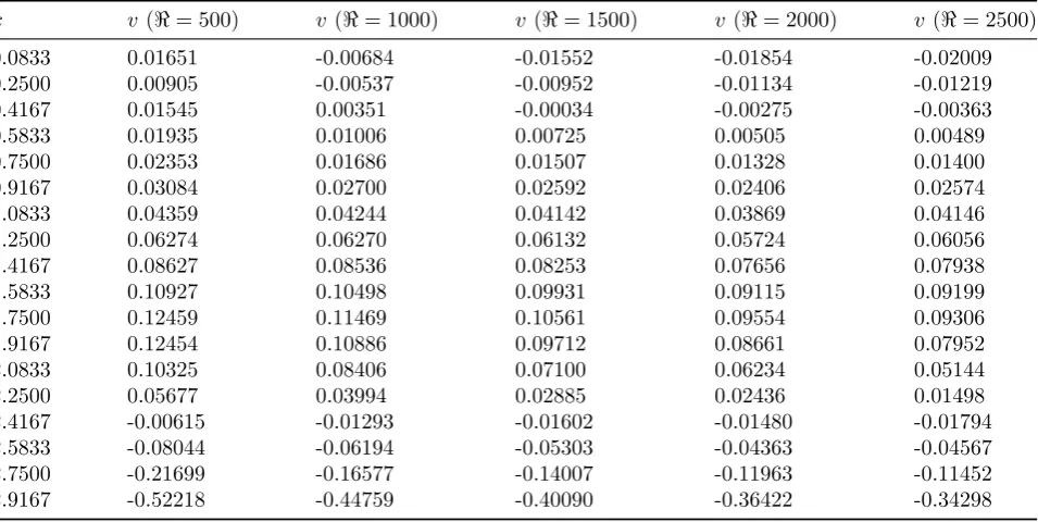
Table 2: Numerical solutions of v-velocity curves along the horizontal line through geometric center of the rectangular domain.
x v (ℜ= 500) v(ℜ= 1000) v (ℜ= 1500) v (ℜ= 2000) v (ℜ= 2500)
0.0833 0.01651 -0.00684 -0.01552 -0.01854 -0.02009
0.2500 0.00905 -0.00537 -0.00952 -0.01134 -0.01219
0.4167 0.01545 0.00351 -0.00034 -0.00275 -0.00363
0.5833 0.01935 0.01006 0.00725 0.00505 0.00489
0.7500 0.02353 0.01686 0.01507 0.01328 0.01400
0.9167 0.03084 0.02700 0.02592 0.02406 0.02574
1.0833 0.04359 0.04244 0.04142 0.03869 0.04146
1.2500 0.06274 0.06270 0.06132 0.05724 0.06056
1.4167 0.08627 0.08536 0.08253 0.07656 0.07938
1.5833 0.10927 0.10498 0.09931 0.09115 0.09199
1.7500 0.12459 0.11469 0.10561 0.09554 0.09306
1.9167 0.12454 0.10886 0.09712 0.08661 0.07952
2.0833 0.10325 0.08406 0.07100 0.06234 0.05144
2.2500 0.05677 0.03994 0.02885 0.02436 0.01498
2.4167 -0.00615 -0.01293 -0.01602 -0.01480 -0.01794
2.5833 -0.08044 -0.06194 -0.05303 -0.04363 -0.04567
2.7500 -0.21699 -0.16577 -0.14007 -0.11963 -0.11452
2.9167 -0.52218 -0.44759 -0.40090 -0.36422 -0.34298
Fw, Fe convective mass flux per unit area at west and east faces respectively, kgm−2s−1
Fs, Fn convective mass flux per unit area at south and north faces respec-tively, kgm−2s−1
Dw, De diffusivity conductance at west and east faces respectively, Wm−2K−1 Ds, Dn diffusivity conductance at south
Table 3: Numerical solutions of (−∂x∂P)along the horizontal linethrough geometric center of the rectangular domain
x ℜ= 500 ℜ= 1000 ℜ= 1500 ℜ= 2000 ℜ= 2500
0.2500 0.00646 0.00450 0.00390 0.00358 0.00314
0.4167 0.00429 0.00336 0.00297 0.00285 0.00254
0.5833 0.00323 0.00214 0.00165 0.00147 0.00122
0.7500 0.00213 0.00101 0.00039 0.00006 -0.00016
0.9167 0.00091 -0.00017 -0.00072 -0.00099 -0.00114
1.0833 0.00001 -0.00085 -0.00114 -0.00143 -0.00117
1.2500 0.00186 0.00131 0.00128 0.00077 0.00177
1.4167 0.01109 0.01020 0.00985 0.00800 0.00994
1.5833 0.03155 0.02797 0.02539 0.02087 0.02295
1.7500 0.06181 0.05132 0.04444 0.03635 0.03727
1.9167 0.09173 0.07150 0.05914 0.04721 0.04554
2.0833 0.10440 0.07540 0.05913 0.04492 0.04059
2.2500 0.08032 0.05317 0.03823 0.02810 0.02223
2.4167 0.02341 0.01048 0.00449 0.00425 -0.00079
2.5833 -0.03978 -0.02448 -0.01886 -0.01365 -0.01468
2.7500 -0.11306 -0.06056 -0.04179 -0.02600 -0.02755
2.9167 -0.18831 -0.12537 -0.09327 -0.08623 -0.06848
Subscript i,j index used in tensor notation nb neighboring coordinate P central grid point
E neighbor in east direction W neighbor in west direction N neighbor in north direction S neighbor in south direction e control volume faceP and E w control volume faceP and W n control volume faceP and N s control volume faceP and S
Figure 1: The rectangular domain.
1
Introduction
T
htransfer in a rectangular domain plays ane problem of coupled fluid flow with heat important role in various equipment and pro-cess of the industry. For example, there is aFigure 2: The staggered grid.
Figure 3: Au-control volume and its neighboring velocity components.
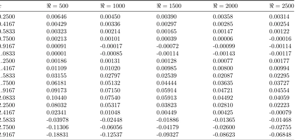
indus-Table 4: Numerical solutions of
(
−∂P ∂y
)
along the vertical linethrough geometric center of the rectangular domain
y ℜ= 500 ℜ= 1000 ℜ= 1500 ℜ= 2000 ℜ= 2500
0.0833 -0.00859 -0.00502 -0.00363 -0.00247 -0.00294
0.1389 -0.00585 -0.00316 -0.00172 -0.00093 -0.00068
0.1944 -0.00576 -0.00212 -0.00033 0.00092 0.00102
0.2500 -0.00513 -0.00099 0.00134 0.00227 0.00353
0.3056 -0.00546 0.00007 0.00253 0.00271 0.00462
0.3611 -0.00593 -0.00004 0.00236 0.00210 0.00427
0.4167 -0.00783 -0.00167 0.00075 0.00042 0.00274
0.4722 -0.01008 -0.00410 -0.00164 -0.00190 0.00041
0.5278 -0.01287 -0.00711 -0.00464 -0.00432 -0.00230
0.5833 -0.01536 -0.01000 -0.00750 -0.00644 -0.00514
0.6389 -0.01712 -0.01227 -0.00994 -0.00810 -0.00743
0.6944 -0.01751 -0.01383 -0.01165 -0.00920 -0.00949
0.7500 -0.01654 -0.01510 -0.01308 -0.01015 -0.01090
0.8056 -0.01386 -0.01540 -0.01354 -0.01057 -0.01157
0.8611 -0.00938 -0.01251 -0.01239 -0.01020 -0.01063
0.9167 -0.00448 -0.00525 -0.00672 -0.00741 -0.00754
0.9722 -0.00335 -0.00335 -0.00259 -0.00297 -0.00278
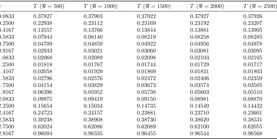
Table 5: Numerical solutions of temperature along the horizontal line through geometric center of the rectan-gular domain
x T (ℜ= 500) T (ℜ= 1000) T (ℜ= 1500) T (ℜ= 2000) T (ℜ= 2500)
0.0833 0.37827 0.37903 0.37922 0.37927 0.37926
0.2500 0.22938 0.23112 0.23169 0.23192 0.23207
0.4167 0.13557 0.13766 0.13844 0.13881 0.13905
0.5833 0.07944 0.08140 0.08219 0.08258 0.08285
0.7500 0.04709 0.04859 0.04922 0.04956 0.04978
0.9167 0.02933 0.03021 0.03060 0.03081 0.03095
1.0833 0.02068 0.02089 0.02098 0.02103 0.02105
1.2500 0.01818 0.01767 0.01744 0.01729 0.01717
1.4167 0.02058 0.01929 0.01869 0.01831 0.01803
1.5833 0.02796 0.02576 0.02472 0.02406 0.02359
1.7500 0.04154 0.03829 0.03673 0.03574 0.03505
1.9167 0.06396 0.05952 0.05738 0.05603 0.05510
2.0833 0.09975 0.09419 0.09150 0.08981 0.08870
2.2500 0.15654 0.15034 0.14735 0.14549 0.14432
2.4167 0.24723 0.24157 0.23881 0.23710 0.23601
2.5833 0.39238 0.38908 0.38730 0.38620 0.38531
2.7500 0.62024 0.62086 0.62089 0.62100 0.62055
2.9167 0.96094 0.96335 0.96455 0.96544 0.96568
try, heat exchanger, wind loaded structure, in-ternal combustion engine. Since the primary at-tractive feature of the control volume method is that it is a method to represent and evaluate partial differential equations in the form of al-gebraic equations. Ghiaet al. [12] have used the vorticity-stream function formulation of the
Table 6: Numerical solutions of temperature along the vertical line through geometric center of the rectangular domain
y T (ℜ= 500) T (ℜ= 1000) T (ℜ= 1500) T (ℜ= 2000) T (ℜ= 2500)
0.0278 0.00216 0.00200 0.00193 0.00188 0.00185
0.0833 0.00643 0.00595 0.00573 0.00557 0.00549
0.1389 0.01051 0.00972 0.00935 0.00910 0.00896
0.1944 0.01427 0.01319 0.01269 0.01235 0.01215
0.2500 0.01759 0.01625 0.01563 0.01521 0.01496
0.3056 0.02034 0.01879 0.01807 0.01759 0.01730
0.3611 0.02243 0.02073 0.01994 0.01943 0.01909
0.4167 0.02378 0.02201 0.02118 0.02065 0.02029
0.4722 0.02437 0.02259 0.02175 0.02122 0.02085
0.5278 0.02418 0.02247 0.02165 0.02115 0.02077
0.5833 0.02324 0.02165 0.02089 0.02042 0.02006
0.6389 0.02160 0.02019 0.01950 0.01908 0.01875
0.6944 0.01932 0.01813 0.01754 0.01718 0.01687
0.7500 0.01650 0.01555 0.01506 0.01477 0.01451
0.8056 0.01324 0.01252 0.01215 0.01193 0.01172
0.8611 0.00963 0.00916 0.00891 0.00875 0.00860
0.9167 0.00583 0.00556 0.00542 0.00533 0.00525
0.9722 0.00194 0.00186 0.00181 0.00178 0.00176
Figure 4: A v-control volume and its neighboring velocity components.
grid. The steady incompressible Navier-Stokes equations in a 2-D driven cavity were solved by Bruneau and Jouron [5] in primitive variables by means of the multigrid method. A finite volume solution method for the two-dimensional Navier-Stokes equations and temperature equation with 4th order discretization on Cartesian grids was presented by Lilek and Peric [16]. Kim and Choi [15] presented a second-order time-accurate nu-merical method for solving unsteady incompress-ible Navier-Stokes equations on hybrid unstruc-tured grids. Kalita et al. [14] have proposed a higher order compact (HOC) finite difference so-lution procedure for the steady two-dimensional convection-diffusion equations on non-uniform or-thogonal Cartesian grids. Piller and Stalio [20] used the staggered grid arrangement to study one
and two-dimensional simulations for the scalar transport and Navier-Stokes equations.
Ben-Figure 5: Scalar control volume (continuity equa-tion).
Figure 6: u-velocity curves along the vertical line through geometric center of the domain.
Navier-Figure 7: v-velocity curves along the horizontal line through geometric center of the domain.
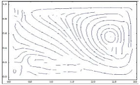
Figure 8: Steady-state contours for stream lines forℜ= 1000.
Stokes equations on staggered grids. Basak and Chamkha [3] considered heat line analysis on nat-ural convection for nanofluids confined within square cavities with various thermal boundary conditions. Garoosi et al. [7] reported a study about the natural convection heat transfer of the nanofluid in a square cavity with several pairs of heaters and coolers (HACs) inside.
They found that location of the heater and cooler (HAC) has the highest impact on the heat transfer rate. Chamkha and Ismael [6] analyzed conjugate heat transfer in a porous cavity filled with nanofluids and heated by triangular thick wall. Garoosi et al. [8] studied the natural con-vection and mixed concon-vection of the nanofluid in a square cavity using Buongiorno model. Garoosi et al. [9] have numerically studied natural con-vection heat transfer of nanofluid in a 2-D square cavity containing several pairs of heater and cool-ers (HACs). Garoosi et al. [10] have carried out a numerical study concerning natural and mixed convection heat transfer of nanofluid in a 2-D square cavity with several pairs of heat source-sinks using the finite volume method. Garoosi et al. [11] have used two phase mixture model for numerically investigating the problem of steady state mixed convection heat transfer of nanofluid in a two-sided lid driven cavity with several pairs of heaters and coolers (HACs) inside.
The literature survey pertinent to coupled fluid
Figure 9: Steady-state contours for stream lines forℜ= 500.
Figure 10: Steady-state contours for stream lines forℜ= 1500.
Figure 11: Steady-state contours for stream lines forℜ= 2000.
Figure 12: Steady-state contours for stream lines forℜ= 2500.
a fully coupled fluid flow with heat transfer in a rectangular domain. We have used this method to solve the governing equations along with slip wall boundary conditions.
The summary of the layout of the current
Figure 13:
( −∂P
∂x
)
along the horizontal line
through geometric center of the rectangular do-main.
work is as follows: Section 2 provides the gov-erning equations of a viscous incompressible fluid flow with heat transfer and the boundary con-ditions for the rectangular domain. Section 3
describes the control volume method under nu-merical method. Section 4 describes numerical computations along with the SIMPLE algorithm. Section5discusses the numerical solutions of the flow variables, steam lines and isotherms of the flow. Section 6 illustrates the conclusions of this study.
2
Problem Formulation
2.1 Physical Description
The geometry of the problem in the paper along with the boundary conditions is drawn in
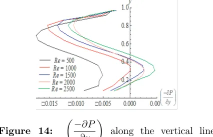
Fig-Figure 14:
( −∂P
∂y
)
along the vertical line
through geometric center of the rectangular do-main.
ure 1. ABCD is a rectangular domain about the point (1.5,0.5) in which steady 2-D incompress-ible viscous flow is considered. Flow is setup in a rectangular domain with three stationary walls and a top lid that moves to the right with con-stant speed (u= 1). At all four corner points of the computational domain velocity components are assumed to vanish. It may be noted here regarding specifying the boundary conditions for pressure, the convention followed is that either the pressure at the boundary is given or velocity component normal to the boundary is specified.
2.2 Governing equations
dimensionless form can be written as follows:
Continuity equation ∂u
∂x + ∂v
∂y = 0, (2.1)
x-momentum equation
u∂u ∂x+v
∂u ∂y =−
∂P ∂x +
(
1 ℜ
)(
∂2u ∂x2 +
∂2u ∂y2
)
,
(2.2)
y-momentum equation
u∂v ∂x+v
∂v ∂y =−
∂P ∂y +
(
1 ℜ
)(
∂2v
∂x2 +
∂2v
∂y2
)
,
(2.3)
Energy equation
u∂T ∂x +v
∂T ∂y =
1 Pr
(
∂2T ∂x2 +
∂2T ∂y2
)
. (2.4)
Figure 15: Temperature along the horizontal line through geometric center of the domain.
Figure 16: Temperature along the vertical line through geometric center of the domain.
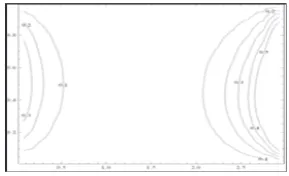
Figure 17: Isotherms forℜ= 500.
Figure 18: Isotherms forℜ= 1000.
2.3 Boundary conditions
The slip wall and temperature boundary condi-tions are given by:
on boundary AB: u= 0, ∂v
∂x = 0, T = 0, on boundary BC: u= 0, v = 0, T = 0,
on boundary CD: u= 0,∂v
∂x = 0, T = 1, on boundary AD:u= 1, v= 0, T = 0.
(2.5)
3
Numerical Method
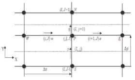
The numerical method that has been adopted for the problem under study is the Control Volume Method (CVM) based on a uniform staggered grid system. In a staggered grid [21, pp. 195-200] as shown in Figure2, the scalar variables, in-cluding pressure, are stored at the nodes marked (•). The velocities are defined at the (scalar) cell faces in between the nodes and are indicated by arrows. Horizontal arrows indicate the locations for u-velocity and the vertical ones denote those for v-velocity. In addition to the E, W, N, S notation, the u-velocity are stored at cell faces e and w and the v-velocity at cell faces n and s. We observe that the control volumes for u and v are different from the scalar control volumes and from each other. The scalar control volumes are sometimes referred to as the pressure control volumes because the discretized continuity equa-tion is turned into a pressure correcequa-tion equaequa-tion, which is evaluated on scalar control volumes.
Figure 19: Isotherms forℜ= 1500.
letters. . . , i−1, i, i+1, . . .and. . . , j−1, j, j+1, . . . in the x-and y-directions respectively. A sub-script system based on this numbering allows us to define the locations of grid nodes and cell faces with precision. Expressed in the new co-ordinate system, the discretizedx-momentum equation at the location (i, J) is given by:
ai,J ui,J = Σanbunb+ (PI−1,J −PI,J)Ai,J. (3.6)
WhereAi,Jis the (east or west) cell face area of
Figure 20: Isotherms forℜ= 2000.
the u-control volume. In the numbering system theE,W,N andSneighbors involved in the sum-mation Σanbunbare (i−1, J), (i+ 1, J), (i, J−1) and (i, J + 1). Their locations and the prevail-ing velocities are shown in the Figure 3. The coefficients for hybrid differencing scheme are as follows:
Figure 21: Isotherms forℜ= 2500.
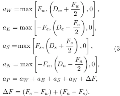
aW = max
[
Fw,
(
Dw+ Fw
2
)
,0
]
,
aE = max
[
−Fe,
(
De− Fe
2
)
,0
]
,
aS= max
[
Fs,
(
Ds+ Fs
2
)
,0
]
,
aN = max
[
−Fn,
(
Dn− Fn
2
)
,0
]
,
aP =aW +aE+aS+aN + ∆F,
∆F = (Fe−Fw) + (Fn−Fs).
(3.7)
The coefficients contain combinations of the con-vective flux F and the diffusive conductance D atu-control volume cell faces. Applying the new notation system we give the values of F and D for each of the facese,w,nandsof theu-control volume.
Fw = (u)wAw=
Fi,J+Fi−1,J 2
= 1
2[ui,JAi,J+ui−1,JAi−1,J],
Fe= (u)eAe=
Fi+1,J +Fi,J 2
= 1
2[ui+1,JAi+1,J +ui,JAi,J],
Fs= (v)sAs=
FI,j+FI−1,j 2
= 1
2[vI,jAI,j+vI−1,jAI−1,j],
Fn= (v)nAn=
FI,j+1+FI−1,j+1
2
= 1
2[vI,j+1AI,j+1+vI−1,j+1AI−1,j+1],
Dw = 1
ℜ∆x, De = 1
ℜ∆x, Ds= 1 ℜ∆y,
Dn= 1 ℜ∆y.
(3.8)
By analogy the y-momentum equation becomes
aI,j vI,j= Σanbvnb+ (PI,J−1−PI,J)AI,j. (3.9)
The pressure correction equation is given by:
aI,JPI,J′ =aI+1,JPI′+1,J +aI−1,JPI′−1,J +aI,J+1PI,J′ +1+aI,J−1PI,J′ −1
+b′I,J. (3.10)
Where
aI,J =aI+1,J +aI−1,J +aI,J+1+aI,J−1,
aI+1,J = (dA)i+1,J,
aI−1,J = (dA)i,J,
aI,J+1= (dA)I,j+1,
aI,J = (dA)I,j,
di,J = Ai,J
ai,J
, dI,j = AI,j
aI,j ,
b′I,J = (u∗A)i,J−(u∗A)i+1,J
+(v∗A)I,j −(v∗A)I,j+1.
(3.11)
Finally, the temperature discretized equation
aPTP =aWTW +aETE+aSTS+aNTN. (3.12)
Where
aW= max
[
Fw,
(
Dw+ Fw 2 ) ,0 ] ,
aE= max
[
−Fe,
(
De− Fe 2 ) ,0 ] ,
aS= max
[
Fs,
(
Ds+ Fs 2 ) ,0 ] ,
aN= max
[
−Fn,
(
Dn− Fn 2 ) ,0 ] ,
aP=aW +aE +aS+aN + ∆F,
∆F = (Fe−Fw) + (Fn−Fs).
(3.13)
(3.14)
Fw =ui,J, Fe=ui+1,J,
Fs=vI,j, Fn=vI,j+1,
Dw = 1
Pr ∆x, De= 1 Pr ∆x,
Ds= 1
Pr ∆y, Dn= 1 Pr ∆y.
4
Numerical Computations
We have obtained the numerical computations of the four unknown flow variablesu,v,P, andT by using the discretized equations (3.6), (3.9), (3.10) and (3.12) respectively. The input data, for the relevant parameters in the governing equations like Reynolds number (ℜ) and Prandtl number (Pr), has been properly chosen by considering physical significance of the present problem. To compute the numerical solutions, we have used the SIMPLE algorithm. We have executed the algorithm with the aid of a computer program developed and run in C-complier. The acronym SIMPLE stands for Semi-Implicit Method for Pressure-Linked Equations. The algorithm is originally put forward by Patankar and Spalding [21] and essentially a guess-and correct procedure for the calculation of pressure on a staggered grid arrangement introduced above. We preferred to use the SIMPLE algorithm that gives a method of calculating pressure and velocities. The method is iterative, and when other scalars are coupled to the momentum equations the calculation needs to be done sequentially. The discretized momen-tum equations and pressure correction equation are solved implicitly; where the velocity correc-tion is solved explicitly. This is the reason why it is called “Semi-Implicit Method”. The algo-rithm involves aniterative process in which the pressure correction equation is susceptible to di-vergence unlesssome under-relaxation is used. We have used a suitable under-relaxation factor to find outthe converged values of pressure and ve-locities.
4.1 The SIMPLE Algorithm
The SIMPLE algorithm for solving coupled fluid flow and heat transfer consists of the following steps:
velocities:
PI,J=PI,J∗ +PI,J′ ,
ui,J=u∗i,J+di,J(PI′−1,J−PI,J′ ),
vI,j=vI,j∗ +dI,j(PI,J′ −1−PI,J′ ).
(4.15)
Solve the temperature discretized equations. Replace the previous in-termediate values of pressure and ve-locity (u∗, v∗, P∗, T∗) until the corrected values (u, v, P, T)return to Step 2 and repeat this process until the solution converges.
The pressure correction equation (3.10) is also prone to divergence unless some under-relaxation is used. So we underrelaxu∗, v∗ while solving the momentum equation (with a relaxation factorα), further we employ
PI,J =PI,J∗ +αPPI,J′
.
5
Numerical Results and
Dis-cussion
We have used the control volume method de-scribed under section 3 to carry out the nu-merical computations of velocity, pressure and temperature. We have summarized this method under SIMPLE algorithm described under sec-tion 4. In order to get clear insight into the problem, the numerical computations of veloc-ity, pressure gradients and temperature for ℜ = 500,1000,1500,2000,2500 and Pr = 7.0 have been done based on the method described un-der Section3 along with the algorithm given un-der Section 4.1. The behavior of fluid flow vari-ables which are horizontal and vertical compo-nents of velocity, pressure gradients and temper-ature has been described by using the numeri-cal solutions given under Tables1–6. In Table1, we list out the numerical solutions for u-velocity curves at different Reynolds numbers (ℜ = 500, 1000, 1500, 2000, 2500), along the vertical line through geometric center of the rectangular do-main. Its behavior has been illustrated in Fig-ure6. We observed that, for a givenℜ,u-velocity
first decreases from the bottom boundary (u= 0) value and then, gradually increases up to the up-per boundary (u = 1) value. We also observed that, the absolute value of u-velocity decreases with increase in Reynolds number. The near-linearity of u-velocity curves in the central core of the rectangular domain can also be observed. Similarly, Table 2 shows the numerical solutions for v-velocity curves at different Reynolds num-bers (ℜ = 500,1000,1500,2000,2500). Figure 7
illustrates the behavior ofv-velocity curves along the horizontal line, through the geometric cen-tre of the rectangular domain. It is evident that, for a given ℜ, v-velocity increases initially and then decreases after attaining its extremum value. Further, the absolute value ofv-velocity decreases with increase in Reynolds number. Figures 8-12
display steady-state contours for the stream lines for ℜ = 500,1000,1500,2000,2500. The origin for these contours for various Reynolds numbers (ℜ) has been displayed for clarity of the veloc-ity curves. The recirculating nature of the fully developed flow induced due to the moving upper wall is seen vividly inside the rectangular domain. The point of zero velocity represents the center around which the general body of the fluid ro-tates in the rectangular domain. This center is located in the direction of the moving boundary. The effect of the velocity of the upper wall on the fluid inside the rectangular domain diminishes as we move away from the upper wall boundary. The numerical solution for(−∂x∂P)along the horizontal line of the rectangular domain has been given in Table 3. In Figure 13 we illustrate the behavior of (−∂x∂P) for
ℜ= 500,1000,1500,2000,2500
. We observed that
(
−∂P ∂x
)
is increasing initially and then decreases after at-taining its extremum value. In Table 4, the nu-merical solution for
(
−∂P ∂y
)
be-havior of
( −∂P
∂y
)
for
ℜ= 500,1000,1500,2000,2500
. We observed that
( −∂P
∂y
)
is increasing near boundaries and decreases inside the domain. We also observed that (−∂x∂P) and
( −∂P
∂y
)
both de-creases with the increment in ℜ. The numer-ical solutions of temperature profile, for ℜ = 500,1000,1500,2000,2500 and for Pr = 7.00, have been given under Table 5 and 6. Figure 15
illustrates the behavior of T along the horizontal line through the geometric centre of the rectan-gular domain. Figure 16 illustrates the behavior ofT along the vertical line through the geometric centre of the rectangular domain. These figures are depicting a comparison of the heat transfer from the wall CD towards the wall AB and from the wall BC towards the wall AD of the rectan-gular physical domain considered. The isotherms contours have been drawn to illustrate the fluid flow behavior inside the rectangular domain. It can be observed that high temperature generated at the right and left wall boundaries extended to-wards the middle of the rectangular domain.
6
Conclusions
The problem of a steady 2-D incompressible, vis-cous flow with heat transfer with slip wall bound-ary conditions in a rectangular domain has been investigated. A control volume method, with hy-brid scheme has been employed as a numerical scheme to solve the governing equations of this problem. The well-known SIMPLE algorithm is employed for velocity, pressure and temperature coupling. The numerical computations for these flow variables have been obtained by employing the SIMPLE algorithm which has been imple-mented with the help of a code in C-programming language. In this study, Reynolds numbers (ℜ) = 500,1000,1500,2000,2500 have been considered. Prandlt number (Pr) = 7.0, which physically cor-respond to water, has been consider for this study. We observed that, the absolute value of velocity profile decreases with increase in Reynolds num-ber. The recirculating nature of the fully devel-oped flow induced due to the moving upper wall is seen vividly inside the rectangular domain. The
effect of the velocity of the upper wall on the fluid inside the rectangular domain diminishes as we move away from the upper wall boundary. We also observed that (−∂x∂P) and
( −∂P
∂y
)
both de-creases with the increment in ℜ. The figures, re-lated to temperature profile, are depicting a com-parison of the heat transfer from the wall CD to-wards the wall AB and from the wall BC toto-wards the wall AD of the rectangular physical domain considered. The isotherm contours inside the do-main depicted that high temperature generated at the right and left boundaries extended towards the middle of the domain.
Acknowledgements
The authors acknowledge the support from the Research Council, University of Delhi for pro-viding Research and Development Grant 2014-15 vide letter no. RC/2014/6820 to carry out this work.
References
1. 2. 3. 4. 5. 6.
[1] J. D. Anderson, Computational Fluid Dynamics with Basics and Applications, McGraw-Hill, New York, 1995.
[2] D. A. Anderson, R. H. Pletcher, J. C. Tan-nehill, Computational Fluid Mechanics and Heat Transfer,Second ed., Taylor and Fran-cis, Washington D. C., 1997.
[3] T. Basak, A. J. Chamkha, Conjugate nat-ural convection in a square enclosure with inclined thin fin of arbitrary length, Inter-national Journal of Heat and Mass Transfer 55, 5526-5543 (2012).
[4] A. Ben-Nakhi, A. J. Chamkha, Conjugate natural convection in a square enclosure with inclined thin fin of arbitrary length, Inter-national Journal of Thermal Sciences 46 (2007) 467-478.
[6] A. J. Chamkha, M. A. Ismael, Conjugate heat transfer in a porous cavity filled with nanofluids and heated by triangular thick wall, International Journal of Thermal Sci-ences 67 (2013) 135-151.
[7] F. Garoosi, G. Bagheri, F. Talebi, Numerical simulation of natural convection of nanoflu-ids in a square cavity with several pairs of heaters and coolers (HACs) inside, Interna-tional Journal of Heat and Mass Transfer67 (2013) 362-376.
[8] F. Garoosi, S. Garoosi, K. Hooman, Nu-merical simulation of natural convection and mixed convection of the nanofluid in a square cavity using Buongiorno model, Pow-der Technology 268 (2014) 279-292.
[9] F. Garoosi, L. Jahanshaloo, M. M. Rashidi, A. Badakhsh, M. E. Ali, Numerical simula-tion of natural convecsimula-tion of the nanofluid in heat exchangers using a Buongiorno model, Applied Mathematics and Computation 254 (2015) 183-203.
[10] F. Garoosi, B. Rohani, M. M. Rashidi, Two phase simulation of natural convection and mixed convection of the nanofluid in a square cavity, Powder Technology 275 (2015) 239-256.
[11] F. Garoosi, B. Rohani, M. M. Rashidi, Two-phase mixture modeling of mixed convection of nanofluids in a square cavity with inter-nal and exterinter-nal heating,Powder Technology 275 (2015) 304-321.
[12] U. Ghia, K. N. Ghia, C. T. Shin, High-resolutions for incompressible flow using the Navier-Stokes equations and a multigrid method, Journal of Computational Physics 48 (1982) 387-411.
[13] A. Hokpunna, M. Manhart, Compact fourth-order finite volume method for numeri-cal solutionsof Navier-Stokes equations on staggered grids, Journal of Computational Physics 229 (2010) 7545-7470.
[14] J. C. Kalita, A. K. Dass, D. C. Dalal, A transformation-free HOC scheme for steady
convection-diffusion on non-uniform grids, International Journal for Numerical Meth-ods in Fluids 44 (2004) 33-53.
[15] D. Kim, H. Choi, A second-order time-accurate finite volume method for unsteady incompressible flow on hybrid unstructured grids,Journal of Computational Physics162 (2000) 411-428.
[16] Z. Lilek, M. Peric, A fourth-order finite vol-ume method with collocated variable ar-rangement,Computers and Fluids 24 (1995) 239-252.
[17] M. L. Mansour, A. Hamed, Implicit solution of the incompressible Navier-Stokes equa-tions on non-staggered grid,Journal of Com-putational Physics 86 (1990) 147-167.
[18] S. V. Patankar, Numerical Heat Transfer and Fluid Flow,Hemisphere, New York, 1980.
[19] R. Peyret, T. D. Taylor, Computational Methods for Fluid Flow, Springer-Verlag, New York, 1983.
[20] M. Piller, E. Stalio, Finite-volume compact schemes on staggered grids,Journal of Com-putational Physics 197 (2004) 299-340.
[21] H. K. Versteeg, W. Malalsekra, An Introduc-tion to ComputaIntroduc-tional Fluid Dynamics: The Finite Volume Method,Second ed. Pearson, India, 2007.
Mohit Kumar Srivastava is Ph.D. in Computational Fluid Dynam-ics from University of Delhi, India. He earned his M.Sc. (Mathemat-ics) from Indian Institute of Tech-nology Kanpur, India and B.Sc. from University of Allahabad, In-dia. His Research interests include CFD, Numer-ical Analysis, NumerNumer-ical solutions of PDEs.