Estimation of Software Reliability by Sequential Testing with Simulated Annealing of Mean Field Approximation

ESTIMATION OF SOFTWARE RELIABILITY BY

SEQUENTIAL TESTING WITH SIMULATED ANNEALING

OF MEAN FIELD APPROXIMATION

Nidhi Gupta and Manu Pratap Singh*

Department of Computer Science, Institute of Basic Science Khandari, Dr. B. R. A. University, AGRA, India

[email protected]

*Corresponding Author

(Received: July 29, 2004 – Accepted: November 2, 2006)

Abstract Various problems of combinatorial optimization and permutation can be solved with neural network optimization. The problem of estimating the software reliability can be solved with the optimization of failed components to its minimum value. Various solutions of the problem of estimating the software reliability have been given. These solutions are exact and heuristic, but all the exact approaches are of considerable theoretical interest. In this paper, we propose the simulated annealing technique of mean field approximation for finding the possible minimum number of failed components in the sequential testing. These minimum numbers of failed components are depending upon the selection of time intervals or slots. The selection of time intervals or slots satisfies all the necessary constraints of the problem. The new energy function with the mean field approximation is also proposed. The constraint parameter for the annealing schedule is also dynamically defined that is changed with the selection of a time interval or slot on each iteration of the processing. The algorithm of the whole process shows that this approach can generate the optimal solution.

Key Words Software Reliability, Mean Field Approximation, Simulated Annealing, Optimization

ﻩﺪﻴﮑﭼ

ﻲﻣ ﺍﺭ ﻲﺒﻴﺗﺮﺗ ﻭ ﻲﺒﻴﻛﺮﺗ ﻱﺯﺎﺳ ﻪﻨﻴﻬﺑ ﻒﻠﺘﺨﻣ ﻞﺋﺎﺴﻣ ﻞـﺣ ﻲﺒﺼـﻋ ﻱﺎـﻫ ﻪﻜﺒﺷ ﻂﺳﻮﺗ ﻱﺯﺎﺳ ﻪﻨﻴﻬﺑ ﺎﺑ ﻥﺍﻮﺗ

ﺩﺮﻛ . ﻤﺨﺗ ﻪﻟﺎﺴﻣ

ﻲﻣ ﺩﺎﻤﺘﻋﺍ ﺖﻴﻠﺑﺎﻗ ﻦﻴ

ﺩﻮـﺷ ﻞـﺣ ﻥﺁ ﻢﻤﻴـﻨﻴﻣ ﺭﺍﺪﻘﻣ ﺎﺗ ﺏﻮﻴﻌﻣ ﺀﺍﺰﺟﺍ ﻱﺯﺎﺳ ﻪﻨﻴﻬﺑ ﺎﺑ ﺪﻧﺍﻮﺗ .

ﻱﺎـﻫ ﻩﺍﺭ

ﺖﺳﺍ ﻩﺪﺷ ﻩﺩﺍﺩ ﺭﺍﺰﻓﺍ ﻡﺮﻧ ﺩﺎﻤﺘﻋﺍ ﺖﻴﻠﺑﺎﻗ ﻦﻴﻤﺨﺗ ﻱﺍﺮﺑ ﻲﻔﻠﺘﺨﻣ .

ﻡﺎـﻤﺗ ﺎـﻣﺍ ﺪﻨﺘﺴـﻫ ﻱﺭﺎـﻜﺘﺑﺍ ﻭ ﻖـﻴﻗﺩ ﺎـﻫ ﺦﺳﺎﭘ ﻦﻳﺍ

ﻲﻣ ﻥﺍﻭﺍﺮﻓ ﻪﻗﻼﻋ ﺩﺭﻮﻣ ﻱﺮﻈﻧ ﺕﺭﻮﺻ ﻪﺑ ﻖﻴﻗﺩ ﻱﺎﻫ ﺵﻭﺭ ﺷﺎﺑ

ﻨ ﺪ . ﺵﻭﺭ ﻪﻟﺎﻘﻣ ﻦﻳﺍ ﺭﺩ ﺩﻻﻮـﻓ ﻥﺪﺷ ﺩﺮﺳ ﻱﺯﺎﺳ ﻪﻴﺒﺷ

ﻱﺍﺮﺑ ﻂﺳﻮﺘﻣ ﻥﺍﺪﻴﻣ ﺐﻳﺮﻘﺗ ﻪﺑ ﻁﻮﺑﺮﻣ ﻪـﺋﺍﺭﺍ ﻲـﺒﻴﺗﺮﺗ ﻱﺎـﻫ ﻥﻮﻣﺯﺁ ﺭﺩ ﺏﻮﻴﻌﻣ ﺀﺍﺰﺟﺍ ﺯﺍ ﺩﺍﺪﻌﺗ ﻞﻗﺍﺪﺣ ﻥﺩﺭﻭﺁ ﺖﺳﺪﺑ

ﻲﻣ ﺩﻮﺷ . ﻞﻗﺍﺪﺣ ﻦﻳﺍ

ﺏﺎﺨﺘﻧﺍ ﻪﺑ ﺏﻮﻴﻌﻣ ﺀﺍﺰﺟﺍ ﺯﺍ ﺩﺍﺪﻌﺗ

ﺘﺴﺑ ﻲﻧﺎﻣﺯ ﻪﻠﺻﺎﻓ ﺩﺭﺍﺩ ﻲﮕ

. ﺏﺎﺨﺘﻧﺍ ﻲﻧﺎﻣﺯ ﻪﻠﺻﺎﻓ )

ﺭﺎﻴـﺷ ﺎـﻳ

ﻲﻧﺎﻣﺯ ( ﻪﻟﺎﺴﻣ ﻡﺯﻻ ﻱﺎﻫ ﺖﻳﺩﻭﺪﺤﻣ ﻪﻴﻠﻛ

ﻲﻣ ﻩﺩﺭﻭﺁﺮﺑ ﺍﺭ ﺩﺯﺎﺳ

. ﻂـﺳﻮﺘﻣ ﻥﺍﺪـﻴﻣ ﺐـﻳﺮﻘﺗ ﻱﺍﺮﺑ ﻱﮊﺮﻧﺍ ﺪﻳﺪﺟ ﻊﺑﺎﺗ ﻚﻳ

ﺖﺳﺍ ﻩﺪﺷ ﻪﺋﺍﺭﺍ ﺰﻴﻧ .

ﻪﻣﺎﻧﺮﺑ ﻱﺍﺮﺑ ﺖﻳﺩﻭﺪﺤﻣ ﺮﺘﻣﺍﺭﺎﭘ "

ﻥﺪﺷ ﺩﺮﺳ " ﺎـﺑ ﻪـﻛ ﻱﺭﻮﻃ ﻪﺑ ﻩﺪﺷ ﻒﻳﺮﻌﺗ ﺎﻳﻮﭘ ﺕﺭﻮﺻ ﻪﺑ ﺰﻴﻧ

ﻲﻧﺎﻣﺯ ﻪﻠﺻﺎﻓ ﺏﺎﺨﺘﻧﺍ )

ﻲﻧﺎﻣﺯ ﺭﺎﻴﺷ ﺎﻳ (

ﻲﻣ ﺮﻴﻴﻐﺗ ﺪﻨﻳﺁﺮﻓ ﺯﺍ ﺭﺍﺮﻜﺗ ﺮﻫ ﺎﺑ ﺪﻨﻛ

. ﻥﺎﺸﻧ ﺪﻨﻳﺁﺮﻓ ﻡﺎﻤﺗ ﻢﺘﻳﺭﻮﮕﻟﺍ ﻲﻣ

ﻪـﻛ ﺪـﻫﺩ

ﻲﻣ ﻩﻮﻴﺷ ﻦﻳﺍ ﺪﻨﻛ ﺩﺎﺠﻳﺍ ﺍﺭ ﻪﻨﻴﻬﺑ ﺦﺳﺎﭘ ﺪﻧﺍﻮﺗ

.

1. INTRODUCTION

Most of the traditional problems of combinatorial permutation can be solved with the help of the Artificial Neural Network [1]. There are various applications and uses of a neural network [2]. One of the most successful applications of the neural network is solving optimization problems [3]. There are many situations where a problem may be

statistical terms as “the probability of fault free operation of a system or component to perform its required functions under stated conditions for a specified period of time” [4]. Software reliability represents a user (or customer) oriented view of software quality. It relates directly to operation rather than design of a program, and hence it is dynamic rather than static. For this reason software reliability is interested in failures occurring and not faults in a program. Failures mean a function of the software that does not meet user requirements .The reliability of any software can be estimated using the failure data of the system, but prediction of exact failures in software is complicated. We have various statistical methods [5] for predicting failures but research indicates that these models are not appropriate for prediction of failure. It may be a better idea to use the optimization technique of ANN for determining the failures and use it for estimating the software reliability.

Various solutions for such types of problems have been proposed in which the problems can be formulated as the optimization of the cost or function with the satisfaction of certain constraints. The same method can also be applied to optimize the reliability estimation, where the objective is to minimize the number of failed components in sequential testing [6-7]. The traditional method to solve such problems was gradient decent approaches of hill climbing and a stochastic simulated annealing [8].

In this paper, we propose the simulated annealing technique of mean field approximation for optimizing the possible minimum number of failed components in the given time duration. The selection of time intervals or slots satisfies all the necessary constraints. Energy function for any Hopfield type feedback neural network represents the stored input pattern in the form of the number of failed components. This energy function also satisfies all the necessary constraints imposed in the problem. A global constraint in the form of the number of failed components in the particular slot or time interval (that is being selected randomly) can be selected for the Annealing schedule. The constraints can be reduced as per annealing schedule and the corresponding the new energy function is estimated. It can be seen that the possible minimum energy function will represent the minimum number of failed components in the

sequential testing.

2. SIMULATED ANNEALING OF MEAN FIELD APPROXIMATION FOR OPTIMIZING

THE NUMBER OF FAILED COMPONENTS OF THE SOFTWARE

of the testing. The weight matrix format can be found from the number of failed components in that particular slot. The output will be labeled as Txi, where the ‘X’, subscript refers to the slot and

the ‘i’, subscript refers to the position in the testing. To formulate the connection weight matrix, the energy function must be constructed so that it satisfies the following criteria:

Energy minima must favor states that have each slot only once in the sequential testing.

Energy minima must favor states that have each position in the testing only once.

Energy minima must favor states with the minimum total number of failed components.

Denoting the state of a processing unit of the Hopfield network as Txi = 1 indicates that the slot

X is to be completed at the ith _{stage of testing, the}

energy function can be written as;

∑∑ ∑

= = = ≠ + = N 1 X N 1 i N 1 j , 1 j X XiT j T 2 A E +

∑ ∑ ∑

= = = ≠ N 1 i N 1 X N X Y , 1 Y Y XiT i T 2 B ) T T ( T f 2 C 1 i, Y 1 i, Y X N 1 X N X Y , 1 Y N 1 i

xy i + −

= = ≠ =

+

∑ ∑ ∑

(2.1) where A, B and C are the positive constants and

denote the relative importance given to the constraints.

The mean field approximation algorithm

[

9-10] also proposed a solution for this type of optimization. The following energy function with a mean field approximation can be proposed:

∑∑∑

≠ + = N i N i j N X X X max

ST ₂ T iT j f E

(

)

∑ ∑ ∑

≠ − + N X N X Y N i 1 i Y, i Y, X

XYT T T

f 2

1

i

(2.2) Where fmax is real constant, which is slightly larger

than the largest number of failed components

between the time intervals in the given sequential testing. There fore, in Equation 2.2, there are only two terms, the first term is regarding feasibility, which inhibits two slots from being in the same testing time. The second summation term is used for the minimization of the number of failed components. The term fmax is used for the

balancing of the summation terms.

The output Txi of a neuron (X, i) is interpreted

as the probability of finding slot X in testing duration at position i. The mean field for a neuron (X, i) is defined according to the energy function given in Equation 2.2 as;

∑

∑

≠ + − ≠ + + = N X Y 1 i , Y 1 i , Y XY N X Y X max

x f T f (T T )

E _{i i} (2.3)

Initially all the neurons are arranged to the average value and the constraint parameter F with the fmax.

The weights of the interconnections are initialized with small random numbers. As per the Hopfield model, the stable state of the any ith neuron can be define as

∑

≠ = + i j j j i '

i(t 1) F [ W T (t) ]

T (2.4)

This stable state may lead to a state corresponding to a local minimum of the energy function. In order to reach the global minimum, i. e. the possible minimum number of failed components in the sequential testing, by passing the local minima, we use the concept of stochastic updating of the unit in the activation dynamics of the network. In stochastic updating, the state of units is updated using the probabilistic updating, which is controlled by the annealing schedule constraint parameter (F = fmax) and the probability

distributions of the states at thermal equilibrium is given as;

F / E Xi _Ze Xi

1 ) T (

P = − (2.5)

Where Z is the partition function.

components i. e. to its higher value. So at a higher F, many states are likely to be visited, irrespective of the energies of those states. Now, the value of the constraint parameter F is gradually reduced as per the annealing schedule, and the output value of the states perturb. This perturbation continues until the network settles in to a stable state or equilibrium state. So, the network estimates the energy function for this state and compares it with the previous energy function by computing ΔE. If

ΔE ≤ 0, we accept the solution with the highest probability i.e. 1, otherwise we accept it with the probability given in the Equation 2.5. On each iteration of this process, the solution is accepted with the probability 1, and then the constraint parameter F is assigned with fmax of the newly

constructed energy function. Then every time on the acceptable solution with higher probability, the constraints parameter changes with the newly found maximum number of failures. This newly found maximum number of failed components will be less then the previously found maximum number of failed components. So the simulated annealing process will continue with the new value of the constraint parameter. This process continues until the final value of the schedule is obtained. At this state the units of the network represent the state of equilibrium, which will represent the minimum energy function for the network. Thus the minimum energy function will represent the possible minimum number of failed components in the sequential testing.

In order to speed up the process of the simulated annealing, the mean field approximation is used, in which the stochastic updating of the binary units is replaced by deterministic analog states. Thus the fluctuating activation value of each unit is replaced with its average value. The Equation 2.4 can be express with this method as:

∑

∑

≠ ≠ > < = > < = > + < i j j ij ' i j j j i '

i(t 1) F[ W T(t) ] F W T(t)

T (2.6)

and from the stochastic updating with thermal equilibrium we have;

∑

≠ > < = > + < N i j j ij

i _F W T (t) ]

1 [ tanh ) 1 t (

T (2.7)

This equation is solved iteratively starting with

some arbitrary values < Ti (0) > initially. The stable

state in the mean field approximation is a result of minimization of an effective energy and defined as the function of F:

] T ) T ( E F 1 [ tanh T i i i _{∂ < >}

> < ∂ − = >

< (2.8)

Where the effective energy E (< Ti >) is the

expression for energy function of the Hopfield model using averages for the state variables.

Now the constraint parameter F decreases as per the annealing schedule, the state of the network perturbs with the stochastic asynchronous updating of the processing elements. So, as the output value perturbs, the neurons produce the updated states. The states updating continues until the Equation 2.6 satisfied.

Hence, for stable conditions the energy function of the annealing schedule can be expressed as;

∑∑∑

≠ + > >< < = N i N i j N X X X new max

ST ₂ T i T j f E (2.9)

(

)

∑ ∑ ∑

≠ − > + < > < N X N X Y N i 1 i Y, i Y, X

XY T T T

f 2

1

i

The energy difference ΔE is computed as;

∑ ∑

≠ > < = − = N i N i j new X new max old ST new

ST ₂ T i

f E E E Δ + > < > < − >

<

∑ ∑

≠ old X N i N i j old X old max new

Xj ₂ T i T j f T

∑ ∑ ∑

≠ > − < − N X N X Y N i old X new X old XY new

XY f )( T T ) f ( 2 1 i i

(

)

(

)

[

old

]

1 i, Y 1 i, Y new 1 i, Y 1 i,

Y T T T

T + > − < + >

< _{+ − + −}

(2.10)

F / E mp e

P α −Δ On each iteration with the highest probability of accepting the solution, the constraint parameter of the Annealing Schedule is defined as;

new max f

F= (2.11)

On each iteration, the constraint parameter is changed to its minimum value with respect to the previous value. Hence, each time the network determines the stable condition with the new value of energy function E and constraints parameter F (when PE < = 0). The neurons produce the stable state that represents the position of the slot with a minimum number of failed components with respect to the previous position. So, at stable condition with ΔE ≤ 0 the state of the neurons can be defined from the Equation 2.5

new max i f 1 [ tanh Tx >= − < ] T i X N i N i j N X N X N X Y N i ] ) 1 i Y, T 1 i Y, T ( i X T Y X f 2 1 j Tx i x T 2 f [ new max > < ∂ <

∑∑∑

∑∑∑

≠ ≠ > − + + < > < + > < > ∂ (2.12)

The Mean field for the neuron (X, i), where output < TXi > can be interpreted as the probability of

finding the slot X in the ith _{testing position as}

defined from the Equation 2.3 as;

∑

∑

≠ ≠ + − > + < + > < = N X Y N X Y 1 i , Y 1 i , Y XY X new max

X f T f ( T T )

E _{i i}

(2.13)

Thus, the entire process continues until a fixed point is found for the every value of constraint parameter F. In the process of selecting a fixed point, change in the energy is computed and the probability of accepting the point in the minimum number of failed components can be found. The field for the selected points will also be computed. This entire process will continue for every schedule of the constraints parameter F, until F reaches the final value.

The algorithm of the entire process can be

proposed as:

Initialize the weights and bias with a small random number. The value of F is initialized with any large random number.

Store the input pattern in the form of the number of failed components (f₁,f₂,−−−,f_n) that are observed during the different time slots i.e. (Δt₁,Δt₂,−−−,Δt_n) of sequential testing for the different modules of the software. The number of failures (f₁,f₂,−−−,f_n) is stored with the stable state of the network as:

∑

≠ = + i j j ij '

i(t 1) F[ WT(t)] T

Do until the fixed point is found. Randomly select a slot say X. Compute the energy function as;

∑∑∑

≠ + > >< < = N i N i j N X X X max

ST ₂ T i T j f E

(

)

∑ ∑ ∑

≠ − > + < > < N X N X Y N i 1 i Y, i Y, X

XY T T T

f 2

1

i

Compute the state of the unit at equilibrium;

] T E f 1 tanh[ Tx i X ST max

i _{∂< >}

∂ −

>= <

Also calculate the ΔEusing Equation 2.7: if ΔE ≤ 0 accept with P < TXi >

(accept) _{= 1 and set F}

= fmax else P < TX_i >(accept) = exp (ΔE/F)Compute

the Mean field as

∑

≠ + − > + < + > < = N X Y 1 i , Y 1 i , Y XY X max

i f T f ( T T )

Ex _i

(The average of the output values of accepted fixed point i. e. neurons).

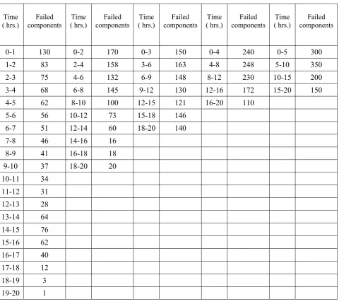
TABLE 1. Number of Failures in the Different Time Intervals for the Sequential Testing.

Time ( hrs.)

Failed components

Time ( hrs.)

Failed components

Time ( hrs.)

Failed components

Time ( hrs.)

Failed components

Time ( hrs.)

Failed components

0-1 130 0-2 170 0-3 150 0-4 240 0-5 300 1-2 83 2-4 158 3-6 163 4-8 248 5-10 350

2-3 75 4-6 132 6-9 148 8-12 230 10-15 200

3-4 68 6-8 145 9-12 130 12-16 172 15-20 150

4-5 62 8-10 100 12-15 121 16-20 110

5-6 56 10-12 73 15-18 146

6-7 51 12-14 60 18-20 140

7-8 46 14-16 16

8-9 41 16-18 18

9-10 37 18-20 20

10-11 34 11-12 31 12-13 28 13-14 64 14-15 76 15-16 62 16-17 40 17-18 12 18-19 3 19-20 1

annealing schedule and repeats Step 2.

3. SIMULATION RESULTS

In this paper, for estimating the software reliability we have applied the technique of sequential testing with simulated annealing of mean field approximation. The pattern of failure

0 50 100 150 200 250 300 350 400

0 5 10 15 20 25

Time Interval (hrs.)

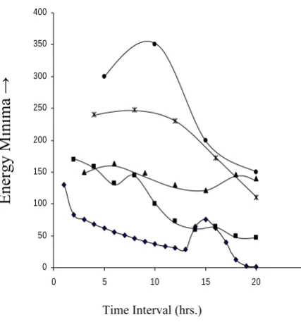
Figure 1. Number of failures at different time interval at

different energy minima’s.

results obtained are tabulated as shown in Table 1.

This table lists the total number of failed components at the end of 1hr, 2 hr, 3hr, etc. in the second column. In the same manner, the total number of failed components at the end of 2hr, 4hr, etc. are listed. The same pattern can be seen in the following columns. Now after some iteration this number of failures will be stored in different energy minima’s with the time interval (as Figure 1 shows) according to this energy function as given in Equation 2.2.

Initially the arbitrary slot is selected and the energy function is constructed as given in Equation 2.2. The annealing schedule is assigned with the maximum number of failures i.e. F. At the higher F, many states are likely to be seen. Therefore, the value of the constraints parameter F is gradually reduced as per the annealing schedule, the output value of the state perturbs. This perturbation continues until the network settles to a stable state or an equilibrium state.

At the stable state after minimizing the constraint parameter, Table 2 can be constructed.

Table 2 shows the results

that the number of

TABLE 2. Selection of Time Interval with the Minimum Number of Failures.

Time interval Number of Failures

0-1 130 0-2 0-3 0-4 0-5 1-2 83 2-3 75 2-4 3-4 68 3-6 4-5 62 4-6 4-8 5-6 56 5-10

6-7 51 6-8 6-9 7-8 46 8-9 41 8-10 8-12 9-10 37 9-12 10-11 34 10-12 10-15 11-12 31 12-13 28 12-14 12-15 12-16 13-14 64 14-15 14-16 65 16-17 40 16-18 16-20 17-18 12 18-19 3 18-20 19-20 1

Energy Minima

failures of 130 gradually reduces from its higher values of 350. This trend continues in the other rows for the selection of the next slots. Now the energy function will change as given in Equation 2.10 and the state of the neurons can be defined in Equation 2.5.

This entire process will continue for every schedule of the constraint parameter F, until F reaches the final state. After completing the entire iterations for the allowed minimum limit of F, Table 3 can be constructed.

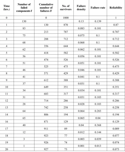
Table 3 shows that, the number of failed components has been reduced. Initially we have 1,000 failures and after applying the annealing schedule in the sequential testing, 927 cumulative numbers of failures remain. The results of the fourth column shows that this technique of optimization reduced 73 failed components.

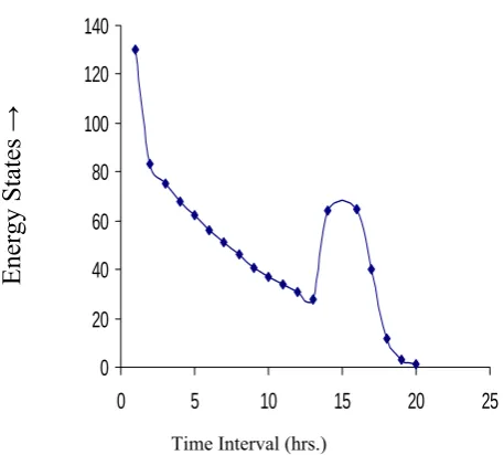
Figure 2 shows the optimized number of failed components with different time intervals in the energy landscape. This table also shows the failed component density, failed component intensity, and the reliability after getting the failures in each time interval. The table shows that the reliability of software components increases.

4. CONCLUSIONS

In the process of estimating the software

reliability we are optimizing the failed

software components to their minimum value.

Using the simulated annealing technique of

MFA we reduce the failures in a very

systematic way. For this we divide the total

time duration in the small time intervals or

slots and note the failed components at the end

of each slot.

The selection of time interval or slot

depends upon certain constraints. The main

contribution of our work is to design or

formulations of necessary constraints under

which the slot is selected and determining the

optimized number of failed components of the

software. To accomplish the task of optimizing

the number of failed components, we select the

slots in the sequential testing. The selection of

slots satisfies all the necessary constraints

imposed in the problem.

The Hopfield energy function represents

the stored failed components in different time

intervals in the sequential testing. The

constraint parameter F of the annealing

schedule will change on each iteration of the

process with the fmax (number of failures),

which is slightly

larger than the number of failures between slots that have been selected for the sequence.

This newly found maximum number of failed components will be less then the previously found maximum number of failed components. So the simulated annealing process will continue with the new value of the constraint parameter. This process continues until the final value of the schedule is obtained.

At this state the units of the network represent the state of the equilibrium, which represents the minimum energy state for the network. Thus the minimum energy function will represent the possible minimum number of failed components in the sequential testing. Thus, energy iteration will be scheduled with the optimized value of F.

The reliability of the software is easily estimated with the optimized minimum number of failures determined by the network. The results show that after applying the sequential testing with MFA we can optimize the number of failures up to a minimum value. These minimum numbers of failures increase the software's reliability. More experiments and analytical investigation are still required for increasing the efficiency and speed of the solution.

8. REFERENCES

1. Hassoun, M. H., “Fundamentals of Artificial Neural Networks”, MIT Press, Cambridge, MA, (1995). 2. Wasserman, P. D., “Advanced Method in Neural

Computing”, Van Nostrand Reinhold, New York, NY, (1993).

3. Fogel, D. B., “An Introduction to Simulated Evolutionary Optimization”, IEEE Trans. Neural Network, 5, (1994), 3-14.

TABLE 3. Optimized Value of the Number of Failures, Cumulative Number of

Failures, Failure Rate, Failure Density and the Reliability.

Time (hrs.)

Number of failed components f

Cumulative number of

failures F

No. of survivors

Failure

density Failure rate Reliability

0 0 1000 1

130 0.13 0.139

1 130 870 0.87

83 0.083 0.101

2 213 787 0.787

75 0.075 0.1

3 288 712 0.712

68 0.068 0.1

4 356 644 0.644

62 0.062 0.101

5 418 582 0.582

56 0.056 0.101

6 474 526 0.526

51 0.051 0.101

7 525 475 0.475

46 0.046 0.101

8 571 429 0.429

41 0.041 0.1

9 612 388 0.388

37 0.031 0.1

10 649 351 0.351

34 0.034 0.101

11 683 317 0.317

31 0.031 0.103

12 714 286 0.286

28 0.028 0.103

13 742 258 0.258

64 0.064 0.283

14 806 194 0.194

65 0.065 0.04

16 871 129 0.129

40 0.04 0.368

17 911 89 0.089

12 0.012 0.144

18 923 77 0.077

3 0.003 0.039

19 926 74 0.074

1 0.001 0.013

5. Musa, J. D., Iannino, A. and Okumoto, K., “Software Reliability: Measurement, Prediction, Application, Professional Edition”, Software Engineering Series, McGraw - Hill, New York, NY, (1990).

6. Karunanithi, K., Whitley, D. and Malaiya, Y., “Using Neural Networks in Reliability Prediction”, IEEE Software, 9-4, (1992), 53-59.

7. Traintafyllos, G., Vassiliadis, S. and Kobrosly, W., “On the Prediction of Computer Implementation Faults Via static Error Prediction Models”, Journal of Systems and Software, 28-2, (1995), 129-142.

8. Sharma, N. K., Mangal, M. and Singh, M. P., “Solution of Traveling Salesman Problem with Simulated Annealing of Mean Field Approximation Neural Network”, Proceeding of the Second International Conference on Mathematical and Computational Models, Coimbatore Allied Publishers, (2003), 297-304.

9. Srinath, L. S., “Reliability Engineering”, Affiliated East West Press Pvt. Ltd., (1991).

10. Waterman, R. E. and Hayatt L. E., “Testing - When do I Stop?”, (Invited), International Testing and Evaluation Conference, Washington, DC, USA, (1994).

0 20 40 60 80 100 120 140

0 5 10 15 20 25

Time Interval (hrs.)

Figure 2. The energy states of the optimized number of failed

components.

Energy States