Dataset of Early
Drosophila
Gene Expression
Alexander Spirov
Department of Applied Mathematics and Statistics and The Center for Developmental Genetics, Stony Brook University, Stony Brook, NY 11794-3600, USA
The Sechenov Institute of Evolutionary Physiology and Biochemistry, Russian Academy of Sciences, 44 Thorez Avenue, St. Petersburg 194223, Russia
Email:[email protected]
David M. Holloway
Mathematics Department, British Columbia Institute of Technology, Burnaby, British Columbia, Canada V5G 3H2
Chemistry Department, University of British Columbia, Vancouver, British Columbia, Canada V6T 1Z1 Email:david [email protected]
Received 10 July 2002 and in revised form 1 December 2002
Understanding how genetic networks act in embryonic development requires a detailed and statistically significant dataset in-tegrating diverse observational results. The fruit fly (Drosophila melanogaster) is used as a model organism for studying devel-opmental genetics. In recent years, several laboratories have systematically gathered confocal microscopy images of patterns of activity (expression) for genes governing earlyDrosophiladevelopment. Due to both the high variability between fruit fly embryos and diverse sources of observational errors, some new nontrivial procedures for processing and integrating the raw observations are required. Here we describe processing techniques based on genetic algorithms and discuss their efficacy in decreasing observa-tional errors and illuminating the natural variability in gene expression patterns. The specific developmental problem studied is anteroposterior specification of the body plan.
Keywords and phrases:image processing, elastic deformations, genetic algorithms, observational errors, variability, fluctuations.
1. INTRODUCTION
Functional genomics is an emerging field within biology aimed at deciphering how the blueprints of the body plan en-crypted in DNA become a living, spatially patterned organ-ism. Key to this process is ensembles of control genes acting in concert to govern particular events in embryonic devel-opment. During developmental events, genes encoded in the DNA are converted into spatial expression patterns on the scale of the embryo. The genes, and their products, are active players in regulating this pattern formation. In the first few hours of fruit fly (Drosophila melanogaster) development, a network of some 15–20 genes establishes a striped pattern of gene expression around the embryo [1,2] (Figure 1). These stripes are the first manifestation of the segments which char-acterize the anteroposterior (AP) (head-to-tail) organization of the fly body plan. Similar segmentation events occur in other animals, including humans.Drosophilaresearch helps to understand the genetics underlying such processes.
Though Drosophila may be a relatively easy organism in which to do developmental genetics, there remain many
experimental problems to be resolved. One of these is the processing of large set of gene expression images in order to achieve an integrated and statistically significant detailed view of the segmentation process.
It is not possible to observe all segmentation genes at once in the same embryo over the duration of patterning. Single embryos can be imaged for a maximum of three segmentation genes. Embryos are killed in the fixing pro-cess prior to imaging. Therefore, data sets integrated from multiple embryos, stained for the variety of segmentation genes, and over the patterning period, are necessary for gaining a complete picture of segmentation dynamics. In addition, collecting images from multiple flies (hundreds) allows us to quantitate the level of natural variability in segmentation and the experimental error in collecting this data.
More and more laboratories (including those en-gaged in the Drosophila Genome Project) are present-ing images of embryos from confocal scannpresent-ing, for ex-ample, [3, 4] (see http://urchin.spbcas.ru/Mooshka/ and
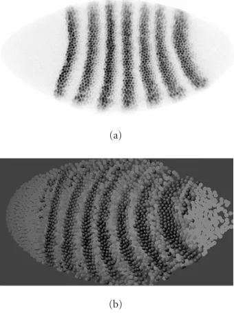
(a)
(b)
Figure1: An example of an expression pattern image and its 3D reconstruction forDrosophila. These images show the first indica-tions of body segmentation in the embryo. (a) An image of a devel-oping fruit-fly egg under light microscope. The egg is shaped like a prolate ellipsoid. Dark dots are nuclei located just under the egg surface. There are about 3000 nuclei in this image. The nuclei are scanned to visualize the amount of one of the segmentation gene products (even-skippedoreve) at each nucleus. The darker the nu-cleus, the greater the local concentration ofeve. (b) A reconstructed 3D picture showing the arrangement of nuclei and visualizing the evepattern in a yellow-red-black palette.
processing challenges in reconstructing expression profiles from the results of confocal microscopy.
In this paper, we review problems in the field of pro-cessing confocal images of Drosophilagene expression and present our processing techniques based on genetic algo-rithms (GAs). We will discuss their efficacy in decreasing ob-servational errors and visualizing natural variability in gene expression patterns.
2. PROBLEMS AND APPROACHES FOR INTEGRATING DATA SETS FROM RAW IMAGES
Sources of variability in our images can be roughly subdi-vided into natural embryo variability in size and shape, nat-ural expression pattern variability, errors of image processing procedures, experimental errors (fixation, dyeing), observa-tional errors (confocal scanning), and the molecular noise of expression machinery.
2.1. Size and shape
Early embryos of isogenic fruit flies can differ in length by 30%. Regardless of such differences in size, expression pat-terns for segmentation remain qualitatively the same. This is a classic case of scaling in biological pattern formation; the
(a)
(b)
Figure 2: Embryos of the same time class and the same length have different expression patterns.Evestripes differ in spacing and overall domain along the anteroposterior (AP, x-) axis, and show stripe curvature in the dorsoventral (DV,y-) direction.
final pattern is not dependent on embryo size (at least within the limits of natural size variability). However, integration of data from different flies requires size standardization.
Size variability was resolved by image preprocessing with theKhorospackage [5]. After a cropping procedure, each im-age was rescaled to the same length and width. Relative units of percent egg length are used.
2.2. Expression pattern variability
Even after cropping and rescaling, there is still variation in the positioning and proportions of expression patterns for the same gene at the same developmental stage (Figure 2).
To match two images such as Figures2aand2b(in or-der to make integrated datasets), we use 2D elastic defor-mations. We treat separately the dorsoventral (DV) curva-ture differences and the AP spacing differences [6]. First, we perform a 2D elastic deformation to straighten segmen-tation stripes. This step minimizes the DV contribution to the AP patterning, especially to AP variability. Next, on a pairwise basis, we move (in 1D) the stripes into regis-ter along the AP axis, minimizing the variability in stripe spacing and overall expression domain. These two steps make for a tough optimization procedure, which is probably best solved with modern heuristic approaches such as GAs [6].
2.3. Scanning error
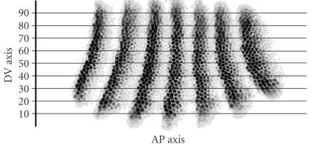
0 0
50 100
DV
ax is%
80 60 40 20 0
AP axis %
Figure3: An example of the systematic DV distortion of an expres-sion surface, with the geneKr¨uppel.
errors which have a systematic character. Due to the ellip-soidal geometry of the egg, nuclei in the center of the image (along the AP axis) are closer to the microscope objective and look brighter than nuclei at the top and bottom of the image. Intensity shows a DV dependence (Figure 3). The brightness depends (roughly) quadratically on DV distance from the AP midline. We flatten this DV bias by a procedure of expression surface stretching.
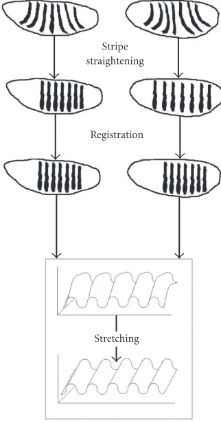
Figure 4summarizes the three steps of image processing which follow the scaling: stripe straightening, stripe regis-tration, and expression surface stretching. The details of the processing techniques are inSection 3.
After image processing, we can generate an integrated dataset and begin to address questions regarding the seg-mentation patterning dynamics. We are pursuing two prob-lems initially. First, we are visualizing the maturation of the expression patterns for all segmentation genes over the pat-terning period. Second, since we have removed many of the sources of variability in the images, what remains should be largely indicative of intrinsic, molecular scale fluctuations in protein concentrations. We are comparing relative noise lev-els within the segmentation signaling hierarchy. These are some of the first tests of theoretical predictions for noise propagation in segmentation signaling [7, 8]. In general, both of these approaches should provide tests of existing the-ories for segment patterning.
3. METHODS
3.1. Confocal scanning of developing Drosophila eggs
Gene expression was measured using fluorescently-tagged antibodies as described in [9]. For each embryo, a 1024×
1024 pixel image with 8 bits of fluorescence data in each of 3 channels was obtained (Figure 5). To obtain the data in terms of nuclear location, an image segmentation procedure was applied [10].
Registration
Stretching
Figure4: Steps for processing large sets of images to obtain an inte-grated dataset of segmentation pattern dynamics (a pair of images used in this example). Stripe straightening minimizes the DV con-tribution to the AP patterning. Stripe registration minimizes the variability in AP stripe positioning. Expression surface stretching minimizes systematic observational errors in the DV direction.
The segmentation procedure transforms the image into an ASCII table containing a series of data records, one for each nucleus. (About 2500–3500 nuclei are described for each image.) Each nucleus is characterized by a unique iden-tification number, thex- and y-coordinates of its centroid, and the average fluorescence levels of three gene products.
At present, over 1000 images have been scanned and pro-cessed. Our dataset contains data from embryos stained for 14 gene products. Each embryo was stained foreve(Figures
1and2) and two other genes.
Time classification
Figure5: An example of an embryo separately dyed and scanned for three gene products.
3.2. Deformations by polynomial series
Our three main deformations introduced above (stripe straightening, registration, and surface stretching) are based on polynomial series. Due to the character of segmenta-tion pattern variability, our deformasegmenta-tions are reminiscent of an earlier attempt by Thompson [12] to quantitatively de-scribe the mechanism of shape change . Stripe straightening looks quite similar to his famous image of a puffer fish to
Mola molafish transformation. This visually simple graphi-cal technique was explicitly described by Bookstein [13,14]. We have found that Drosophila segmentation patterns can also be related by such simple transformation functions.
The stripe-straightening procedure is a transformation of the AP,x-coordinate by the following polynomial:
x=Axy2+Bx2y+Cxy3+Dx2y2, (1)
wherex = w−w0,y = −h−h0,wandhare initial
spa-tial coordinates, andw0,h0,A,B,C, andDare parameters.
They-coordinate remains the same while thex-coordinate is transformed as a function of both coordinateswandh(for details, see [6,15,16]). The parametersw0,h0,A,B,C, and
Dfor each image are found by means of GAs.
Our pairwise image registration procedure is the next step in the sequential transformation of thex-coordinate. We use the following polynomial forx:
x=c
0+c1x+c2x2+c3x3+c4x4+c5x5, (2)
wherec0,c1,c2,c3,c4, andc5are parameters found by means
of GAs for each image (for details, see [6,16]).
Complete registration is achieved by sequential applica-tion of the polynomial transformaapplica-tions (1) and (2) to pairs of images. Complete registration within each time class relative to a starting image (the time class exemplar) gives sets of im-ages suitable for constructing integrated datasets. If we then compare results across time classes, we are able to visualize detailed pattern dynamics over cell cycle 14.
The starting images in each time class, the time class ex-emplars, were chosen using the following way: the distance between each (stripe-straightened) image and every other (stripe-straightened) image in a time class was calculated using the registration cost function (seeSection 3.3). These costs were summed for each image and the image with the lowest total cost was used as the starting image. All other im-ages in the time class were registered to this image. The start-ing image was unaffected by the registration transformation [6].
We perform (fluorescence intensity) surface stretching to decrease DV distortion using the following polynomial:
Z=Z+C
1Y+C2Y2+C3XY+C4Y3+C5XY2+C6X2Y, (3)
whereZis expression,X =w−W0,Y =h−H0,wandh
are initial spatial coordinates, andW0,H0,C
0,C1,C2,C3,C4,
andC5are parameters found by means of GAs. Note thatW0
andH0generally differ fromw0andh0in expression (1).
The computing time for finding parameters by opti-mization techniques is comparable for the three polynomial transformations (1), (2), and (3), though stripe straightening (1) is the most time intensive [6,15,16].
3.3. Optimization by GAs
We tested several techniques for optimization of (1) and (2): GAs, simplex, and a hybrid of these [6,16]. Fitting polyno-mial coefficients is fairly routine and can be solved with any GA library. All we need is to define cost functions for our three particular tasks.
We used a standard GA approach in a classic evolution-ary strategy (ES). ES was developed by Rechenberg [17] and Schwefel [18] for computer solution of optimization prob-lems. ES algorithms consider the individual as the object to be optimized. The character data of the individual is the parameters to be optimized in an evolutionary-based pro-cess. These parameters are arranged as vectors of real num-bers for which operations of crossover and mutation are defined.
AP axis
Figure6: Scheme of image stripping for cost function calculation.
3.3.1 Cost function for stripe straightening
The following procedure evaluates chromosomes during the GA calculation for stripe straightening. Each image was sub-divided into a series of longitudinal strips (Figure 6). Each strip is subdivided into bins, and a mean brightness (local fluorescence level) is calculated for each bin. Each row of means gives a profile of local brightness along each strip. The cost function is computed by pairwise comparison of all profiles and summing the squares of differences between the strips. The task of the stripe-straightening procedure is to minimize this cost function.
3.3.2 Cost function for registration
To evaluate the similarity of a registering image to the refer-ence image (time class exemplar), we use an approach sim-ilar to the previous one. We take longitudinal strips from the midlines of the registering and reference images (e.g.,
Figure 6, centre strip). The strips are subdivided into bins and mean brightness calculated for each bin. Each row of means gives the local brightness profile along each embryo. The cost function is computed by comparing the profiles and summing the squares of differences between them. Registra-tion proceeds until this cost is minimized.
3.3.3 Cost function for surface stretching
To minimize distortion of the (fluorescence intensity) ex-pression surface along the DV direction (y-coordinate), we tested two cost functions based on discrete approximations of first- and second-order derivatives iny:
F1= Zj−Zj+1
2,
F2= 2Zj−Zj+1−Zj−1
2
. (4)
Both functions were applied to a row of expression levels at each nucleus (Z), ranked according to DV position (y -coordinate) while the x-coordinate was ignored. Argument
Zjis a given nucleus’ fluorescence level andZj+1andZj−1are
fluorescence levels for its two nearest (DV) neighbors. Our tests show thatF1is better for our purposes.
3.3.4 Implementation
GA-based programs for our three tasks were implemented both in EO-0.8.5 C++ library [4] for DOS/Windows and
verse observational and experimental errors. Our aim with the image processing is to decrease some of the observational and experimental errors and help distinguish these from the natural variability which we would like to study (i.e., charac-terization of the stochastic nature of molecular processes in this gene network). We will discuss the efficacy of the image processing by comparison of initial and residual variability in our data.
4.1. Stripe straightening and registration
With transformations (1) and (2), we aim at as good a match as possible (by heuristic optimizations) between the data within a time class.Figure 7ashows a superposition of about hundred eve expression surfaces after stripe straightening and registration. (The intensity data is discrete at nuclear res-olution but we display some of our results as continuously interpolated expression surfaces.)
Embryo-to-embryo variability of the expression pattern for the first ten zygotic segmentation genes we are studying is similar to that foreve. Because of the two-dimensionality of the expression surface and the irregularity of nuclear distri-bution, quantitative comparison of this variability is a tough biometric task.
One way to simplify the problem is to compare repre-sentative cross-sections through the expression surface along the midline of an embryo in the AP direction (e.g.,Figure 6, center strip). For all nuclei with centroids located between 50% and 60% embryo width (DV position), expression lev-els were extracted and ranked by AP coordinate. This array of 250–350 nuclei gives an AP transect through the expression surface [19].
Using these transects, we can measure the effect on embryo-to-embryo variability of our processing steps.
Figure 7b shows the variability after rescaling and stripe straightening (before complete registration) for about a hundred eve expression profiles from the 8th time class (Figure 7c). Intensity means at each AP position are shown with error bars (standard deviation). Minimizing stripe spac-ing variability, by registration, reduces the error bars signif-icantly (Figures 7d and7e). In addition to molecular-level fluctuations in gene expression, one of the remaining sources of error in Figures7dand7emay be experimental variabil-ity in intensvariabil-ity (from fixing and dying procedures, as well as variability in microscope scanning), estimated at 10–15% of the 0–255 intensity scale. Normalization of this variability may require both image processing and empirical solutions.
4.2. Expression surface stretching
250
AP position (% egg length)
30
AP position (% egg length) (b)
AP position (% egg length) (c)
AP position (% egg length) (d)
AP position (% egg length) (e)
Figure 7: Superposition of about a hundred images forevegene expression from time class 8 (late cycle 14). (a) Superposition of all eve expression surfaces after the stripe straightening and registration. (b) Variability of expression profiles for geneeve after the stripe-straightening procedure. (c) Mean intensity at each AP position, with standard deviation error bars for the expression profiles from (b). (d) Residual variability for the same dataset after stripe straightening and registration. (e) Mean intensity with standard deviation error bars for the expression profiles from (d). These have decreased significantly with stripe registration. Data for the 1D profiles is extracted from 10% (DV) longitudinal strips (e.g.,Figure 6, center strip). Cubic spline interpolation was used to display discrete data.
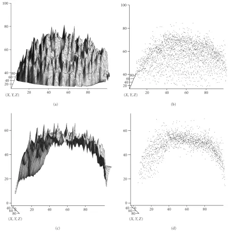
expression surface for such an embryo looks like a half ellip-soid (Figures8aand8b). The fluorescence level at the edges of the image is about 20 arbitrary units, while in the center it
60
40 80 60 40 20
20 40 60 80
(X, Y, Z)
(a)
60
40 80 60 40 20
20 40 60 80
(X, Y, Z)
(b)
60
40
20
0
0 20 40 60 80
40 60
80 (X, Y, Z)
(c)
60
40
20
0
0 20 40 60 80
40 60
80 (X, Y, Z)
(d)
Figure8: Surface stretching transformation. (a) and (b) Experimental expression surface and scatter plot, for a truly uniform distribution of theevegene product. (c) and (d) Expression surface and scatter plot after surface stretching, minimizing the systematic errors in intensity data.
The stretching procedure transforms the expression sur-face along the DV, y-axis (Figures8c and8d). Minimizing the systematic observational error in this direction gives us a chance to directly observe nucleus-to-nucleus variability in a single embryo (Figure 8c).
5. RESULTS AND DISCUSSION
We have found heuristic optimization procedures (transfor-mations (1), (2), and (3)) to be a simple and effective way to reduce observational errors in embryo images. This reduc-tion of variability allows us to focus on the variability
intrin-sic to gene expression and the dynamics of patterning over cycle 14. Here, we give an overview of some of our results with processed datasets.
5.1. Integrated dataset
As mentioned in the introduction, dataset integration from multiple scanned embryos is necessary due to the impossi-bility of simultaneously staining embryos for all segmenta-tion genes at once (the current limit is triple staining). Other work [19, 20] have begun to address the processing nec-essary to standardize images for dataset integration. Myas-nikova et al. [19] have used transects, as in Figures7band
250 200 150 100 50
Fluor
esc
enc
e
30 40 50 60 70 80 90
AP position
20 30
40 50
60
DV positio
n
Figure9: Part of an integrated dataset of gene expression in time class 8 (late cycle 14) for the gap geneshunchback(hb),giant(gt), Kr¨uppel, andknirps(kni) and the pair-rule geneeve. Each surface is the gene expression for a time class exemplar (as discussed in
Section 3).
a different method than ours). Our work adds the steps of stripe straightening and surface stretching, allowing for the construction of 2D expression surfaces and integrated datasets (Figure 9). These steps also minimize contributions to AP variability from DV sources, clarifying the task of studying molecular sources of intensity variability.
More such processed segmentation patterns are posted and updated on the website HOX Pro (http://www.iephb. nw.ru/hoxpro, [21]) and the web-resource DroAtlas (http:// www.iephb.nw.ru/∼spirov/atlas/atlas.html).
5.2. Dynamics of profile maturation
Any analysis of the formation of gene expression patterns must address the striking dynamics over cycle 14. Especially in early cycle 14, these patterns are quite transient, only set-tling down around mid-cycle 14 to the segmentation pattern. Comparative analysis of pattern dynamics for the pair-rule genes is particularly important. Essential questions on the mechanisms underlying these striped patterns are still open [22,23].
The only way to trace the patterning in sufficient detail to address these questions is to integrate large sets of em-bryo images over these developmental stages. (Time rank-ing within cycle 14 is not a simple task. Presently, it takes an expert to rank images into time classes. We are developing automated software for ranking, to be published elsewhere.) AP profiles which have been registered can be integrated into composite pictures like Figure 10, which plots AP distance horizontally against time (at the 8 time class resolution) ver-tically, with intensity in the outward direction.
Figure 10allows us to examine a number of features of cycle 14 expression dynamics. Gap genes tend to establish sharp spatial boundaries earlier than the pair-rule genes. Pair-rule genes are initially expressed in broad domains, which later partition into seven stripes. The regularity of the
gt
hb
kni
eve 1 2 3 4 5 6 7
hairy 1 2 3 4 5 6 7
Figure10: Three-dimensional diagrams representing dynamics of AP profiles of expression for the gap genesgt,hb,kni, and pair-rule geneseve andhairy(h). Horizontal coordinate is spatial AP axis (from left to right); vertical coordinate is time axis (from up to down); expression axis is perpendicular to the plane of the dia-grams. White numbers marks individual stripes ofeveandhairy.
late cycle pattern is well covered in the literature, but the de-tails of the early dynamics are not so well characterized.
All five genes show a movement towards the middle of the embryo, with anterior expression domains moving pos-teriorly and posterior domains moving anpos-teriorly. In more detail, the small anterior domain ofknirps(white arrowhead) appears to move posteriorly at the same speed asevestripe 1 (also marked by white arrowhead). It appears that we can see interactions betweenhbandgtin the posterior: a posterior
gt peak forms first, but as posterior hbforms, the gt peak moves anteriorly. This interaction appears to be reflected in the movement of stripe 7 ofeveandh(black arrowheads).
100
50
0
Fluor
0 20 40 60 80 100
AP position (% egg length) (a)
AP position (% egg length) (b)
Figure11:Eveandbcdfluorescence scatterplots and profiles (early cycle 14, time class 1), sampled from a 50% DV longitudinal strip. (a) Scatterplots after stripe straightening and surface stretching. Each dot is the intensity for a single nucleus. (b) Curves of mean intensity at each AP position, with standard deviation error bars.
5.3. Nucleus-to-nucleus variability
Pictures likeFigure 7cgive us glimpses into the molecular-level fluctuations existing in this gene network. However, such data still displays variability in scanning between em-bryos and over time with the experimental procedure. With stripe straightening and surface stretching, we have a chance to look at nucleus-to-nucleus variability in single em-bryos, eliminating many sources of experimental error. (The drawback is that we are limited to triple-stained embryos.)
Figure 11a shows the maternal proteinbicoid (bcd) (expo-nential) and expression of eve (single peak, the future eve
stripe 1) for a single embryo in early cycle 14. This image was made from a 50% DV longitudinal strip so that the observed variation at any AP position is that in the DV direction (e.g., along a stripe). Each dot is the intensity for a single nucleus. The variation in this plot is largely due to natural, molecular-level fluctuations in gene expression. At this developmental
tional error in the scanned images of segmentation gene ex-pression. Cropping and scaling addresses embryo size vari-ability. Stripe straightening eliminates variable DV contribu-tions to the AP pattern. Registration minimizes differences in expression domains and spacing for pair-rule genes. Expres-sion surface stretching minimizes systematic observational error along the y-axis. The combination of these procedures allows us to create composite 2D expression surfaces for the segmentation genes, allowing us to investigate pattern dy-namics over cycle 14. Also, these procedures allow us to do single-embryo statistics, eliminating many sources of exper-imental variability in order to address molecular-level noise in the genetic machinery.
ACKNOWLEDGMENT
The work of AS is supported by USA National Institutes of Health, Grant RO1-RR07801, INTAS Grant 97-30950, and RFBR Grant 00-04-48515.
REFERENCES
[1] M. Akam, “The molecular basis for metameric pattern in the Drosophilaembryo,” Development, vol. 101, no. 1, pp. 1–22, 1987.
[2] P. A. Lawrence,The Making of a Fly, Blackwell Scientific Pub-lications, Oxford, UK, 1992.
[3] B. Houchmandzadeh, E. Wieschaus, and E. Leibler, “Estab-lishment of developmental precision and proportions in the early Drosophila embryo,”Nature, vol. 415, no. 6873, pp. 798– 802, 2002.
[4] M. Keijzer, J. J. Merelo, G. Romero, and M. Schoenauer, “Evolving objects: a general purpose evolutionary computa-tion library,” inProc. 5th Conference on Artificial Evolution (EA-2001), P. Collet, C. Fonlupt, J.-K. Hao, E. Lutton, and M. Schoenauer, Eds., number 2310 in Springer-Verlag Lecture Notes in Computer Science, pp. 231–244, Springer-Verlag, Le Creusot, France, 2001.
[5] J. Rasure and M. Young, “An open environment for image processing software development,” inProceedings of 1992 SPIE/IS&T Symposium on Electronic Imaging, vol. 1659 of SPIE Proceedings, pp. 300–310, San Jose, Calif, USA, Febru-ary 1992.
[6] A. V. Spirov, A. B. Kazansky, D. L. Timakin, J. Reinitz, and D. Kosman, “Reconstruction of the dynamics of the Drosophila genes from sets of images sharing a common pat-tern,”Journal of Real-Time Imaging, vol. 8, pp. 507–518, 2002. [7] D. Holloway, J. Reinitz, A. V. Spirov, and C. E. Vanario-Alonso, “Sharp borders from fuzzy gradients,” Trends in Ge-netics, vol. 18, no. 8, pp. 385–387, 2002.
[9] D. Kosman, S. Small, and J. Reinitz, “Rapid preparation of a panel of polyclonal antibodies to Drosophila segmentation proteins,” Development Genes and Evolution, vol. 5, no. 208, pp. 290–294, 1998.
[10] D. Kosman, J. Reinitz, and D. H. Sharp, “Automated assay of gene expression at cellular resolution,” inProc. Pacific Sym-posium on Biocomputing (PSB ’98), R. Altman, K. Dunker, L. Hunter, and T. Klein, Eds., pp. 6–17, World Scientific Press, Singapore, 1998.
[11] V. A. Foe and B. M. Alberts, “Studies of nuclear and cyto-plasmic behaviour during the five mitotic cycles that precede gastrulation inDrosophilaembryogenesis,”Journal of Cell Sci-ence, vol. 61, pp. 31–70, 1983.
[12] D. W. Thompson,On Growth and Form, Cambridge Univer-sity Press, Cambridge, UK, 1917.
[13] F. L. Bookstein, “When one form is between two others: an application of biorthogonal analysis,”American Zoologist, vol. 20, pp. 627–641, 1980.
[14] F. L. Bookstein, Morphometric Tools for Landmark Data: Ge-ometry and Biology, Cambridge University Press, Cambridge, UK, 1991.
[15] A. V. Spirov, D. L. Timakin, J. Reinitz, and D. Kosman, “Exper-imental determination of Drosophila embryonic coordinates by genetic algorithms, the simplex method, and their hybrid,” inProc. 2nd European Workshop on Evolutionary Computa-tion in Image Analysis and Signal Processing (EvoIASP ’00), S. Cagnoni and R. Poli, Eds., number 1803 in Springer-Verlag Lecture Notes in Computer Science, pp. 97–106, Springer-Verlag, Edinburgh, Scotland, UK, April 2000.
[16] A. V. Spirov, D. L. Timakin, J. Reinitz, and D. Kosman, “Using of evolutionary computations in image processing for quanti-tative atlas of Drosophila genes expression,” inProc. 3rd Euro-pean Workshop on Evolutionary Computation in Image Analy-sis and Signal Processing (EvoIASP ’01), E. J. W. Boers, J. Got-tlieb, P. L. Lanzi, et al., Eds., number 2037 in Springer-Verlag Lecture Notes in Computer Science, pp. 374–383, Springer-Verlag, Lake Como, Milan, Italy, April 2001.
[17] I. Rechenberg, Evolutionsstrategie: Optimierung technis-cher Systeme nach Prinzipien der biologischen Evolution, Frommann-Holzboog, Stuttgart, Germany, 1973.
[18] H.-P. Schwefel, Numerical Optimization of Computer Models, John Wiley & Sons, Chichester, UK, 1981.
[19] E. M. Myasnikova, A. A. Samsonova, K. N. Kozlov, M. G. Sam-sonova, and J. Reinitz, “Registration of the expression pat-terns of Drosophila segmentation genes by two independent methods,”Bioinformatics, vol. 17, no. 1, pp. 3–12, 2001. [20] K. Kozlov, E. Myasnikova, A. Pisarev, M. Samsonova, and
J. Reinitz, “A method for two-dimensional registration and construction of the two-dimensional atlas of gene expression patterns in situ,” Silico Biology, vol. 2, no. 2, pp. 125–141, 2002.
[21] A. V. Spirov, M. Borovsky, and O. A. Spirova, “HOX Pro DB: the functional genomics of hox ensembles,”Nucleic Acids Re-search, vol. 30, no. 1, pp. 351–353, 2002.
[22] J. Reinitz, E. Mjolsness, and D. H. Sharp, “Model for cooper-ative control of positional information inDrosophilabybicoid and maternalhunchback,” The Journal of Experimental Zool-ogy, vol. 271, no. 1, pp. 47–56, 1995.
[23] J. Reinitz and D. H. Sharp, “Mechanism of eve stripe forma-tion,” Mechanisms of Development, vol. 49, no. 1-2, pp. 133– 158, 1995.
Alexander Spirovis an Adjunct Associate
Professor in the Department of Applied Mathematics and Statistics and the Cen-ter for Developmental Genetics at the State University of New York at Stony Brook, Stony Brook, New York. Dr. Spirov was born in St. Petersburg, Russia. He received M.S. degree in molecular biology in 1978 from the St. Petersburg State University, St. Pe-tersburg, Russia. He received his Ph.D. in
the area of biometrics in 1987 from the Irkutsk State University, Irkutsk, Russia. His research interests are in computational biol-ogy and bioinformatics, web databases, data mining, artificial in-telligence, evolutionary computations, animates, artificial life, and evolutionary biology. He has published about 80 publications in these areas.
David M. Holloway is an instructor of
mathematics at the British Columbia Insti-tute of Technology and a Research Associate in chemistry at the University of British Columbia, Vancouver, Canada. His research is focused on the formation of spatial pat-tern in developmental biology (embryol-ogy) in animals and plants. Topics include the establishment and maintenance of dif-ferentiation states, coupling between