Aircraft Demand Forecasting

www.ijtrd.com

Aircraft Demand Forecasting

1

Rajneesh Singh and

Nikita Jain,

1,2

Career Point University, Alaniya, Rajasthan, India

Abstract - This thesis aims to forecast aircraft demand in the aerospace and defense industry, specifically aircraft orders and deliveries. Orders are often placed by airline companies with aircraft manufacturers, and then suddenly canceled due to changes in plans. Therefore, at some point during the three-year lead time, the number of orders placed and realized deliveries may be quite different. As a result, orders and deliveries are very difficult to predict and are influenced by many different factors. Among these factors are past trends, macroeconomic indicators as well as aircraft sales measures. These predictor variables were analyzed thoroughly, and then used with time series and multiple regression forecasting methods to develop different forecasts for quarterly and annual orders and deliveries. The relative accuracies of forecasts were measured and compared through the use of Theil’s U statistic. Finally, a linear program was used to aggregate multiple forecasts to develop an optimal combination of all forecasts. In conclusion, the methods employed in this thesis are quite effective and produce a wholesome aggregate forecast with an error that is generally quite low for a forecasting task as challenging as this one.

I. INTRODUCTION

In general, forecasting techniques can be broken down into two different categories: qualitative or quantitative. Quantitative forecasting techniques consist of either time series analysis or causal models and rely heavily on historical data. Holt’s Method, moving averages, and trend projection are just a few examples of time series techniques. Causal methods consist of many different regression models. To contrast, qualitative forecasting techniques are much less methodical and rely on judgment. Some examples are the Delphi Method and sales force composites.

The goal of this thesis is to forecast aircraft demand in the aerospace and defense industry, specifically orders and deliveries. Orders are often placed by airline companies with aircraft suppliers and then suddenly canceled due to changes in plans. Therefore, at some point during the three-year lead time, the number of orders and deliveries becomes much different. Thus, orders and deliveries are very difficult to predict, and much analysis must be done in order to forecast these variables adequately.

II. METHODS TO MEASURE FORECAST ACCURACY A. Time Series Methods

Methods for forecasting originated in the 1950s to 1960s and typically did not address the random component of a time series. The main idea was to develop methods for predicting the variable in question from its past data. Some of the simplest univariate forecasting methods are the naïve no-change method, naïve no-change and naïve seasonal no-change method.

𝒏𝒂ï𝒗𝒆𝒏𝒐 − 𝒄𝒉𝒂𝒏𝒈𝒆: Ŷ_𝑡+1= 𝑌_𝑡

𝒏𝒂ï𝒗𝒆𝒄𝒉𝒂𝒏𝒈𝒆: Ŷ𝑡+1= 𝑌𝑡+ (𝑌𝑡− 𝑌𝑡−1)

𝒏𝒂ï𝒗𝒆𝒔𝒆𝒂𝒔𝒐𝒏𝒂𝒍𝒄𝒉𝒂𝒏𝒈𝒆:Ŷ_𝑡+1 = 𝑌_𝑡+ (𝑌_{𝑡+1−𝑠}− 𝑌_𝑡−𝑠)

Another method commonly used to forecast is the simple moving-average method.

In contrast to the naïve method which typically is successful when the observations are relatively constant over time, the moving average method can be used to smooth data in order to see the trend. The forecast is calculated as follows:

Ŷ𝑡+1=

𝑌𝑡+ 𝑌𝑡−1+ 𝑌𝑡−2+. . . +𝑌𝑡−(𝑘−1)

𝑘

Where k is the number of values in the average.

Typically for quarterly data, the k value would be 4, for monthly data the k value would be 12. Typically, the larger the value of k, the smoother is the series.

B. Regression Models

The first forecasting model that is of interest here is linear trend regression. This assumes a contemporaneous relationship between the dependent variable 𝑌_𝑡 and the independent variable t. α0 and α1 are parameter estimates and are estimated

by the method of least squares and ε𝑡 is a random disturbance with zero expected value and constant variance. Parameter estimates for 𝛼₀and 𝛼₁ are 𝑎₀and 𝑎₁.

𝑌𝑡 = 𝛼0 + 𝛼1𝑡 + 𝜀𝑡

𝑌𝑡+1 = 𝑎0 + 𝑎1(𝑡 + 1)

C. Evaluating Forecast Accuracy

There are multiple ways to assess the accuracy of a forecast. Each technique involves comparing the forecasted value with the realized value of a variable of interest. The amount by which the forecast differs from the actual value 𝑌_𝑡 is the forecast error 𝑒𝑡,

Where 𝑒_𝑡 = 𝑌_𝑡 − Ŷ_𝑡

Four simple and commonly used measures of forecast accuracy are presented below.

Firstly, the Mean Absolute Error (MAE), also known as the Mean Absolute Deviation (MAD) is as follows where n is the total number of observations for the period.

MAE = 𝒏𝒕=𝟏 𝒆𝟏

𝒏

Second method used often is the Mean Absolute Percent Error (MAPE). The MAPE is a modification of MAD. MAPE looks at the size of the absolute value of the error relative to the actual value itself. MAPE is presented below.

MAPE = 𝒆𝒕

𝒀𝒕 𝒏 𝒕=𝟏

𝒏 × 𝟏𝟎𝟎

The third method for measuring error is Mean Square Error (MSE). This squares the individual errors as follows

MSE = 𝒆𝒕 𝟐 𝒏 𝒕=𝟏

𝒏

www.ijtrd.com

errors may magnify the overall measure of error. Therefore, using MAD can avoid this. When all of the errors are of the same magnitude, RMSE and MSE are most useful

Another, more unfamiliar measure of forecasting performance is Theil’s U developed by Henri Theil

𝑇𝑕𝑒𝑖𝑙′_{𝑠 𝑈 =} 𝑅𝑀𝑆𝐸 𝑜𝑓 𝑎𝑑𝑣𝑎𝑛𝑐𝑒 𝑎𝑝𝑝𝑟𝑜𝑐𝑕

𝑅𝑀𝑆𝐸 𝑜𝑓 𝑛𝑎ї𝑣𝑒 𝑛𝑜. −𝑐𝑕𝑎𝑛𝑔𝑒

If U >1, then the advanced approach has no value because it cannot perform as well as the naïve no change basic method.

If U<1, the advanced approach has more merit. The closer U gets to 0, the better the approach in question is. (Newbold and Bos 1993)

D. Seasonality

Seasonality is defined as “The estimated seasonal is that part of the series which, when extrapolated, repeats itself over any one-year time period and averages out to zero over such a time period”

Combining Forecasts

Combining different forecasts obtained from different but valid forecasting techniques is a common practice for many forecasters. Early researchers such as Bates, Granger, Newbold, Winkler and Makridakis presented significant evidence toward the effectiveness of combining forecasts.

By combining different competing forecasts one can obtain a vastly superior forecast. It is also perceivably less risky in practice to use a combined forecast rather than selecting a single forecast

Forecasting in the Airline Industry

For lack of literature specifically in methods for forecasting aircraft demand (as top competitors such as Airbus and Boeing keep that very private) we will focus on relevant previous research done on forecasting commercial airline demand.

III. METHODOLOGY

The relative input variables will be discussed in greater detail, as well as their anticipated impact on the multiple regression forecast. Additionally, this chapter will explore greater analysis of the input variables will be explored in terms of seasonality, volatility, correlation with one another, and ultimately correlation with orders and deliveries. This analysis will aid in understanding the underlying relationship between the variables to create a more precise forecast.

A. Description of Variables

The following lists of variables were identified by top competitors in the aerospace industry, such as Boeing (2014) and Airbus (2015) as potential drivers of demand. The variables can be grouped into two categories - global macroeconomic indicators and aircraft sales figures - are listed and defined below. All data is for the time period 1995 to 2013, and is in quarterly and annual increments

.

1. Global Macroeconomic Indicators:

GDP-Worldwide: Gross Domestic Product - The monetary value of all the finished goods and services (In 2005 billion).

GDP Growth: Year over year Percent change

Rate of Inflation Worldwide: Percentage; The rate at which the general level of prices for goods and services is rising

Long Term Interest Rate-Worldwide: Average of daily rates, measured as a percentage

Long Term Interest Rate-US: Average of daily rates, measured as a percentage

Jet Fuel Prices: Price per gallon

Crude Oil Prices: West Texas Intermediate Price per barrel

2. Aircraft Sales Figures:

Aircraft Orders: Number of aircraft ordered

Aircraft Deliveries: Number of aircraft actually delivered Aircraft Order Cancellations: Number of aircraft cancelled Aircraft Net Orders: Orders minus Cancellations

Installed Base-Active: Number of aircraft in active use Retirements: Number of aircraft retired

Revenue Passenger Mile (RPM): In Billions, measures of traffic for airline flights; product of the number of revenue-paying passengers aboard the vehicle and the distance traveled

RPM Growth: Year over year Percent change

Available Seat Mile (ASM): In Billions, measure of a flight's revenue-generating abilities based upon traffic; product of number of seats available and the number of miles flown

ASM Growth: Year over year Percent change Load Factor: Percentage (RPM/ASM)

Operating Revenue: In millions, revenue worldwide Operating Profits: In millions, profits worldwide Net Profits: In millions, net profits worldwide

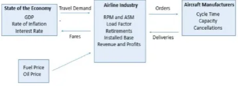
It is expected that as GDP and GDP growth increases, the number of orders and deliveries will increase in kind, as the national wealth increased. Consequently, it is expected that as the fuel price, oil price, rate of inflation and interest rate (in both the U.S. and worldwide) increases, the number of orders and deliveries will decrease due to the increased financial burden.

Aircraft orders and deliveries are linked through aircraft order cancellations. The nature of the aircraft sales industry is such that aircraft are ordered and possibly cancelled during the approximately three-year lead time before delivery. The lead time is not concrete and may take more or less time for an order. Therefore, we cannot simply subtract the number of cancellations from orders three years ago to obtain the number of deliveries in that year. This complicates the problem further; however, we can hypothesize that an increase in the number of cancellations will cause a decrease in the number of deliveries

.

Fig 3.1: Flow Map of the Airline Industry

B. Analysis of Input Variables

1. Seasonality

www.ijtrd.com

data. It is a simple but robust tool for de-seasonalizing data and is therefore sufficient for this analysis. For the quarterly data, a centered moving average of 4 periods at a time was used to eliminate any seasonality, as the data exhibits upswings every 4th quarter of each year. The idea behind a moving average is to smooth out the seasonal variation by taking a rolling average of the data. Then, the seasonal factors are computed by dividing the original data by the averaged data values. Next, an average is taken for each quarter’s seasonal factors to establish one seasonal factor for each of the four quarters. Finally, the original data is divided by the corresponding seasonal factor to generate a de-seasonalized data set.

Fig 3.2: Seasonality of Orders

Fig 3.3: Seasonality of Deliveries

2. Volatility

Volatility is represented as a sliding measure of the coefficient of variation (standard deviation divided by the mean). A time frame of eight quarters was used for the quarterly data, and four years for the annual data. The chart below represents the coefficient of variation for each variable under four different scenarios. The average volatility is measured for both quarterly and annual data. In addition, the volatility of the most recent data (2009-2013) is measured for both quarterly and annual data.

Fig 3.4: Quarterly and Annual Volatility of Input Variables

3. Linear Regression

Linear regression was performed on each input variable against both Orders and Deliveries separately. This was done to evaluate the predicting capacity of each variable as well as to evaluate the predicting ability of both quarterly and annual

data. The tables below summarize the results in order from highest to lowest.

Table 3.1R Squared Values for Input Variables for Orders

Linear Regression for Orders Annual R

Squared

Quarterly R Squared

Net Orders 0.9704 0.9684

Operating Revenue 0.6318 0.3533

ASM 0.6165 0.3438

Fuel Price 0.6174 0.3644

RPM 0.6033 0.3364

Oil Price 0.5781 0.3623

GDP 0.5342 0.2472

Installed Base 0.5310 0.2394

Load 0.4958 0.2756

Cancellations 0.3631 0.2762

Interest Rate US 0.2950 0.1778

Interest Rate Worldwide 0.2561 0.1362

Retirements 0.1520 0.0825

GDP Growth 0.1505 0.0472

RPM Growth 0.0731 0.0428

ASM Growth 0.0345 0.0203

Inflation 0.0157 0.000

Additionally, the figures presented below show an additional view of the R squared values in decreasing order for orders and deliveries.

Fig 3.5. R Squared Values for Orders

Based on this analysis, deliveries seem to be overall easier to predict, as the regression, coefficients are higher than orders for most of the input variables. The variables RPM Growth, GDP Growth, ASM Growth were consequently eliminated from further analysis due to the lack of accurate quarterly data and insignificant correlation to the dependent variables.

Fig 3.6: R Squared Values for Deliveries

IV. ANALYSIS AND RESULTS A. Forecasting Methods and Models

www.ijtrd.com

methods with this data and was the preferred platform for our industry partners. SAS software was used for ARIMA forecasting. It was important to keep this analysis relatively user friendly. Excel is not only user friendly but is relatively inexpensive. Green and Armstrong (2015) focus on similar objectives, keeping the method simple with respect to the forecasting method and the number of input variables.

Regression analysis was recommended as a sound forecasting technique. In addition, it was recommended to use a weighted combination of different forecasts. The following section presents a few different methods for forecasting orders and deliveries. Among them are Holt’s Method, Holt-Winter’s Method, Seasonal Factor Forecasting, Lagged Multiple Regression, and ARIMA forecasting.

1. Naïve No Change Method

To provide a baseline for evaluating more advanced methods, the naïve no change method was used to forecast orders and deliveries. The naïve no-change method simply develops a forecast for the given period (Ŷ_𝑡+1) that is the actual value from the previous period(𝑌𝑡). As rudimentary as this seems,

this provides a baseline for which more sophisticated methods and models should have greater accuracy.

The corresponding naïve no change forecasts for orders and deliveries are presented below. As you can see, the forecast is simply the actual values shifted ahead one period.

Fig 4.1: Naive No Change Forecast for Orders

Fig 4.2: Naive No Change forecast for Deliveries

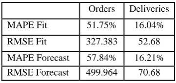
The performance statistics for orders and deliveries are presented in the table below. Again, the Fit values are for the period 1995-2011 and the Forecast values are for the period of 2011-2013.

Table 4.1: Naive No Change Performance Statistics

Orders Deliveries

MAPE Fit 51.75% 16.04%

RMSE Fit 327.383 52.68

MAPE Forecast 57.84% 16.21%

RMSE Forecast 499.964 70.68

2. Holt’s Method

First, Holt’s Method is used on the annual and quarterly data to forecast orders and deliveries. Data from 1995 to 2011 was used to forecast for 2012 and 2013. The actual values for 2012 and 2013 were then compared to the forecasted values. The corresponding graphs for orders are presented below.

Fig 4.3: Holt's Method for Annual Orders

Fig 4.4: Holt's Method for Quarterly Orders

The performance statistics are presented in the table below for both the quarterly and annual forecasts for orders.

Table 4.2: Performance Statistics for Orders Using Holt's Method

Quarterly Annual

MAPE Fit 58.58% 35.93%

RMSE Fit 321.94 1033.27

MAPE Forecast 26.02% 34.10%

RMSE Forecast 315.6 1373.23

3. Holt-Winters Method

Holt-Winters Method was used to accommodate a potential additional factor of seasonality. Holt-Winters method was used explicitly on the quarterly data for orders and deliveries, as minor seasonality was found in both variables during the analysis of input variables. The resulting forecasts for orders and deliveries are presented below.

www.ijtrd.com

Fig 4.6: Holt-Winter's Method for Quarterly Deliveries

Next, the performance statistics for each forecast are presented in the table below.

Table 4.3: Performance Statistics for Orders and Deliveries using Holt-Winter's Method

Orders Deliveries

MAPE Fit 63.31% 12.93%

RMSE Fit 311.46 46.17

MAPE Forecast 29.59% 9.23%

4. ARIMA Forecasting

In this section, SAS software was used to analyze the series and ultimately generate forecasts for orders and deliveries using the Autoregressive Integrated Moving Average (ARIMA) model.

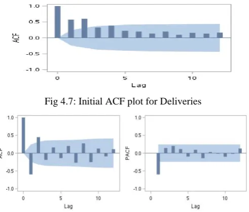
The first step of this analysis is to identify the correct ARIMA model to use for each variable. SAS was used to run a sequence plot of the respective variable. This aids in determining if the series is stationary. Stationarity needs to be achieved before an ARIMA model can be used. In the SAS output presented in the figure below, it is clear that the series for deliveries is non-stationary since its autocorrelation function (ACF) plot decays very slowly.

Fig 4.7: Initial ACF plot for Deliveries

Fig 4.8: ACF and PACF plots for Differenced Deliveries

Since the data is non-stationary, it was first differenced in SAS by taking the logarithm of the data. The figure above displays the autocorrelation function (ACF) plot as well as the partial autocorrelation plot (PACF) for the differenced series. The autocorrelation plot of the differenced series suggests that the series is now stationary. The ACF plot cuts off after the 3rd lag (above the 95% confidence level), therefore this implies that an ARIMA (0,1,2) model could be used. Essentially, when a

plot “cuts off,” it means the lags suddenly cut off after a certain number of lags, and dip lower than the 95% confidence band. However, looking at the PACF, it seems that an ARIMA (1,1,0) model may be sufficient since the lags are not significant past the first one.

Next, the AIC criterion will be used to decide between the two possible models. The AIC values are presented in the table below for both models.

Table 4.4: AIC Values for ARIMA Models for Deliveries

Model AIC Value

ARIMA (1,1,0) 838.698

ARIMA (0,1,2) 842.576

CONCLUSION

A. Overall Performance of Selected Forecasting Models

This thesis implemented different methods and models for forecasting aircraft orders and deliveries. Based on the results presented in the previous section, it is first important to note that all forecasting techniques were deemed more accurate than the Naïve No-Change forecast, according to Theil’s U. This indicates that each forecast is more sophisticated than the most rudimentary method and was sufficient for further analysis.

After aggregation with the Linear Program, it became apparent that the Multiple Regression, Holt-Winters, and ARIMA quarterly forecasts were superior to the Holt and Seasonal Factor forecasts for both Orders and Deliveries, over the forecasting horizon of 8 quarters.

The Multiple Regression model captured the past behavior of the economic indicators for forecasting. It was extremely important to first analyze the input variables for the regression model prior to forecasting, as correlations between predictor variables needed to be identified. Highly correlated input variables can hinder a forecast; therefore, it was important to eliminate highly correlated input variables for the regression analysis.

B. Limitations

This thesis focused on a forecasting horizon of two years, or eight quarters which maintained the relative accuracy of the forecasts given the respective models. However, proceeding further out to a longer forecasting horizon would undoubtedly negatively impact the forecasting accuracy as a whole. Therefore, the aggregate forecasting methods employed in this thesis are limited. More robust machine learning methods could be considered to forecast a longer horizon and are expected to improve accuracy.

References

[1] Green, K.C., Armstrong, J.C., “Simple Forecasting: Avoid Tears before Bedtime”, 2015.

[2] Ho, K. K., “Demand forecasting for aircraft engine aftermarket”, 2008.

[3] Yu, G. (Ed.), “Operations research in the airline industry” (Vol. 9), 2012.

[4] Liehr, M., Größler, A., Klein, M., & Milling, P. M. “Cycles in the sky: understanding and managing business cycles in the airline market”, 2001

[5] Hibon, M., & Evgeniou, T. “To combine or not to combine: selecting among forecasts and their combinations”, 2005.

[6] Fang, Y. “Forecasting combination and encompassing tests”, 2003. [7] Enders, Walter. “Applied Econometric Time Series”, 2004