Cokriging for evaluating agricultural pollution

f

MOIR COPY

tl

W

ter

Proceedings of the Specialty Conference

sponsored by the Irrigation and Drainage Division and the

Water Resources Planning and Management Division of the

American Society of Civil Engineers

and the Delaware Section of ASCE

University of Delaware

Newark, Delaware

July 17-20, 1989

Edited by T. Al Austin

Published by the

American Society of Civil Engineers

345 East 47th Street

APPENDIX - REFERENCES

Bear,

J.

1967. Dynamics

of

fluids in porous media. Elsevier, New York.

Glass, R.J., T. S. Steenhuis and J.-Y. Parlange. "Finger persistence in homogeneous unsaturated media: theory and verification." Soil Science press).

Matthesz, G., M. Isenbeck, A. Pekdeger, J. Schrater.

1985. "Der Stofftransport im Grundwasser and die Wasse rschutzgebietsrichtlinie W 101." Berichte 7/85. Umweltbundesamt, Berlin.

Parker, J.C. and M.Th. van Genuchten. 1984. ing transport parameters from laboratory tracer experiments." Virginia Agricultural Station Bulletin 84-3.

Rice, R.C., D.B. Jaynes, and R.S. Bowman. 1988.

"Pre-ferential Flow of solutes and herbicides under

ir-rigated fields." ASAE Paper No. 88-2634. American Society of Agricultural Engineers, St. Joseph, MI. 10 pp.

Ritter,

W.F., T.H.

Williams and R.P. Eastburn. 1983. "Sprinkler irrigation

of

corn in Delaware." Delaware Agricultural Experiment Station Bulletin 446.

Ritter, W.F., A.E.M. Chirnside, and R.W. Scarborough. 1987. "Pesticide leaching in a coastal plain

soil."

ASAE Paper

No.

87-2630. American Society

of

Ay,-sicul-tural Engineers, St. Joseph, MI.

Scheidegger, A.E. 1957. "On the theory of flow of mis-cible phases in porous media." proc. IUGG, General Assembly, Toronto 2. pp. 236-242.

Steenhuis, T.S., J. Hagerman, N. Pickering, and W.F. Ritter. 1989.

"Flow

path of pesticides in the Delaware and Maryland portion of the Chesapeake Bay Region." Conference on Ground Water Issues and Solutions in the Potomac River Basin/Chesapeake Bay Region. March 14-16, 1989. George Washington University, Washington, DC. 23 pp.

van der Molen, W.H. 1956. "Desalinization of saline

soils

as a column process."

Soil

Science 81:19-27.

COKRIGING FOR EVALUATING AGRICULTURAL POLLUTION

By H.E. Mullis', J.C. Guitjens 2 , M. ASCE, C.W. Robbins 3

ABSTRACT: Agricultural irrigation is a major non-point source polluter. Evaluating the extent of this type of non-point source pollution requires sampling and analysis of drainage waters. To reduce costs, sampling efficiency is important. Cokriging can be used as a tool for interpolating between sampling times or locations. In this experiment, subsurface drainage data from irrigated lands near Twin Falls, Idaho were used. Total Dissolved Solids and NO 3 -N were selected as variables. The objective was to determine if 50 and 65 percent

of

the measured data could be removed (creating two new data sets) and accurately estimated via cokrigin2 using a variogram model based on the remaining data. Cokriging models were developed using statistical information obtained from variograms of the remaining data. Once accurate models were developed for both the 50 and 65 percent removal cases, estimations were made for the missing data values. One-way analysis of variance and t-tests were used to test whether the means and variances of the estimated values were significantly different from those of the measured values. At the 65 percent removal level, there were significant differences in the means and variances of the estimated and measured values for NO3-N. One way analysis of variance and similarity of variance tests were used to test whether differences between the error values of the modeled and removed

d:Itn

were significant. By using the unedited full set of measured data for variogram modeling none of the tests produced rejections.

1 Grad.Student, Dept. of Range, Wildlife and Forestry, University of Nevada-Reno, Reno, NV 89557

2 Prof. of Irrigation Engineering, Dept of Range, Wildlife and Forestry, University of Nevada-Reno, Reno, NV 89557 3 Soil Scientist, USDA-ARS, Snake River Conservation

Research Center, Kimberly, Idaho 83341 1989.

porous (in

•

COKRIGING FOR EVALUATING AGRICULTURAL POLLUTION 129

128 _{NATIONAL WATER CONFERENCE}

INTRODUCTION

Agricultural irrigation accounts for about 35 percent of all water used in the United States (Holmes 1979). Subsurface flows from irrigated lands often have high concentrations of salts. They may also contain nutrient and organics. These constituents can be harmful to man and animals and pose an environmental hazard.

The Federal Water Quality Control Act Amendments of 1972 started . to, address non-point source pollution (Thronson 1978). Since that time, there has been a push to develop best management practices (BMP's) to abate diffuse pollution. To evaluate BMP's, sampling is required.

Sampling and chemical analyses can be very expensive. An efficient sampling scheme that will adequately monitor water quality should also be cost effective. Modeling and interpolation techniques can be used to reduce the required number of samples. This paper focuses on one sampling and interpolation technique called cokriging.

The objective was to optimize sampling efficiency by reducing sampling frequency and substituting estimates between remaining sample values.

The data were collected on the Twin Falls Canal Company irrigation tract in southern Idaho (Carter, Robbins, Bondurant 1973). The 203,000- acre tract has been irrigated for about 83 years. Irrigation water is diverted from the Snake River at Milner Dam and delivered to the farmers by a system of canals. The soils, which vary in depth from a few inches to fifty feet, are underlain by fractured basalts to depths of several hundred feet. Water infiltration rates are fairly high.

Shortly after irrigation was initiated in 1905, high water tables appeared in localized areas throughout the tract. In order to alleviate the problem, horizontal tunnels, four feet wide by seven feet high, were excavated in the basalts to convey excess drainage water to natural surface drains. In all, forty-nine tunnels were constructed. Drainage water quality is of interest because it is the major source of domestic water and the excess finds its way back to the Snake River.

METHODS

Beginning in spring of 1968, some drainage tunnel outlets were sampled. At seven.of these outlets sampling was continued at one-month intervals for approximately two years. The samples were analyzed for concentrations of NE'', K + , Ca", Mg", Cl-, HCO3-, SO4-S, PO4-P, and NO3-N, temperature, p11, and EC. TDS values were approxi-mated by multiplying the EC values by 0.64. In this paper only NO3-N and TDS concentrations are considered.

Named after a South African mining geologist and statistician D.G. Krige, kriging has been widely used in mining and geology for problems such as ore grade estimation (Davis 1973). Kriging estimates values between sample locations and assesses the probable error associated with the estimates. Data estimation is based on weighted adjacent values. These adjacent values are used in linear combinations to estimate values at the unknown point. The weights are based on the covariance in a sequential data series as a function of separation distance. When more than one variable is considered simultaneously, the kriging technique is called cokriging. In this experiment, i.he data were arranged in a temporal structure and the separation distance is in multiples of four weeks. Eight adjacent values are used

(4 preceding and 4 following) to make estimates.

Since values of the variables should have the same

order of magnitude, normalizing each variable independently may be required. Cokriging requires normally distributed data. If the original data series deviates considerably from a normal distribution, data transformation may provide a more acceptable distribution. Cokriging is a best linear unbiased estimator (BLUE) because it preserves the mean and the variance of the original data.

The covariance information is obtained from the variogram (Figure 1). In addition to the variogram model, the variogram has three principal components: the nugget, the sill, and the range. The model may be spherical, linear or gaussian. The range is the separation distance beyond which the observations are independent. The sill is the variogram variance corresponding with the range.

sill

covariance

r ( h )

•

Variance

h • Separation Distance

6

(h)

nugget (h)

INIMM

FIGURE 1.

h

COKRIGING FOR EVALUATING AGRICULTURAL POLLUTION

130

_{NATIONAL WATER CONFERENCE}

The sill tends to approach the variance of the data. The variogram model together with the nugget, sill, and range define the covariance and constitute the statistical parameters used in the cokriging process. Variograma were produced using computer software (Carr, Myers, Glass 1986). One variogram is produced for each variable and one cross-variogram for each possible pair of variables. The cross-variogram uses the sum of the two variables.

The twenty-six temporal values for the first site were arranged sequentially starting with the first and ending with the last data. The twenty-six values from the second site were arranged sequentially and joined to the first twenty-six and so on. The result was a string of 182 data points. This was done for both the TDS and the NO 3 -N data. Then the data were normalized by dividing all the values/of each variable by that variable's mean value. The original data set was edited by systematically removing 50 percent of the data (i.e., removing every other sampling time).

Two variograms and one cross-variogram of the edited data set were produced and the variogram model, nugget, sill, and range were used in the cokriging process. At

the end of the cokriging output of estimates for original input data, the software prints the average cokriging variance and the mean square error. The average cokriging variance is the average of the squared differences between the error values and the mean error. An error value is the difference between the original input value and the corresponding estimate. The mean square error is the average of the squared differences between original input values and corresponding estimates. The average cokriging variance and the mean square error are used to check the accuracy of the model. If their values are not very close the model fits the data poorly. This problem is a result of inaccurate specification of the variogram parameters. The variogram parameter values (nugget, sill, range) must be changed until the fit is acceptable.

After several iterations, an acceptable model was obtained and estimates of the removed data were made. When an adequate model has been obtained, the errors of the modeled data should be normally distributed about a mean of zero and have a constant variance. When the error is random, the cokriging process is truly an unbiased estimator (David 1977).

The modeling procedure was repeated after removing 65 percent of data. The removal 4as systematic. The first sample time was left and times two and three removed. Time four was left and times five and six were removed and so on throughout the data set.

Two tests were used to evaluate the overall accuracy of the estimates. One-way analysis of variance (ANOVA) was used to compare the estimates and actual values. This

type of test involves the calculation of an F value by simultaneously considering the difference in means and the difference in variances (Johnson 1976). Next, using a t-test, the means of the estimates of the removed data were compared to the means of the measured values to determine if the means were from the same population.

For a more detailed analysis of the estimation accuracy, the error sets were examined. One error set was obtained for the modeled data by calculating the differences between the measured values and their corresponding estimates. Another was obtained in the same manner for the removed data. Based on the assumption that the cokriging model had produced acceptable error values for the modeled data, the error sets of the removed data were then compared to the corresponding error sets of the modeled data.

First ANOVA case indicate a

as opposed to the foregoing procedure 50% and 65% of the data values,

data set was used to develop variogram parameters. Subsequently, 50% and 65% of data points were removed in the same manner as before estimates were made. Error sets were produced for removed data (50 and 65 percent). A third error set produced for the entire data set. Based on the assumption that the cokriging process had produced acceptable error values for the entire data set, cross-validation involved similarity of variance tests in which each of the error sets of the removed data were compared to the error set of the entire data set.

RESULTS AND DISCUSSION

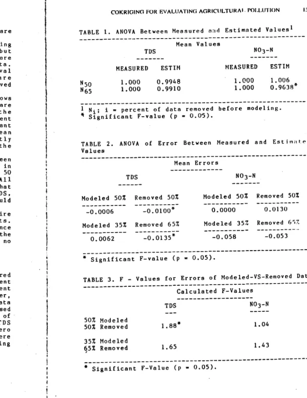
Table 1 shows the results of the ANOVA test between measured and estimated values. Only the NO3-N mean was significant at the 65 percent removal level. The results of the t-test for the means of estimated and actual values were similar. The significant t-value for NO 3 -N at was used. Significant F-values in this

difference in the distribution of the error values about their respective means. Next, a similarity of variance test was used to test for consistency of variance between error sets. This test also involves the calculation of an F-value. However this F-value was based on the variances only.

F = VAR A VARg

VARA and VARB are the variances of the error sets with the larger of the two appearing in the numerator. A significant F-value indicates that the two variances differ.

TABLE 1. ANOVA Between Measured nad Estimated Values 1

Mean Values

TDS NO3-N

1 N .. i = percent of data removed before modeling. Significant F-value (p = 0.05).

TABLE 2. ANOVA of Error Between Measured and Estimated Values

Mean Errors MEASURED ESTIM

1.000 0.9948 1.000 0.9910

MEASURED ESTIM

1.000 1.000 N50

N65

1.006 0.9638 *

I

132 _{NATIONAL WATER CONFERENCE COKRIGING FOR EVALUATING AGRICULTURA}1 PGLIAMON 133

the 65 percent removal level indicates that the means are not representing similar populations.

Table 2 shows the results of the ANOVA test comparing error sets for the modeled data and the measured but removed data. For TDS, the errors of the removed data are significantly different from those of the modeled data. This applies to both the 50 and 65 percent removal levels. These results indicate that the errors are distributed differently between the modeled and removed data series. Therefore the estimates are not reliable.

On the other hand, for NO3-N the ANOVA test shows that the error sets at the 50 percent removal level are not significantly different indicating that the distribution of errors is similar. Even at the 65 percent removal level, the ANOVA test did not show a significant difference between the error sets. However, the mean error of the modeled 35 percent was significantly different from zero indicating an inadequacy in the model.

The results of the similarity of variance test between the errors of the modeled and removed data are shown in Table 3. The variances of the TDS error values at the 50 percent removal level were significantly different. All other variance pairs were similar. However, given that the 50 percent removal results were not ideal for TDS, one must assume that removal of more data (65%) would yield even more unreliable estimates.

The alternative method of using a model of the entire data set to make estimates yielded acceptable results. Table 4 shows the results of the similarity of variance

the entire data set and the removed data. There were no

TDS NO 3 -N

Modeled 50% Removed 50% Modeled 50% Removed 50%

0.0130

Modeled 35% Removed 65% Modeled -35% Removed 657

-0.053 -0.0006 -0.0100 0.0000

0.0062 -0.0135 * -0.058

Significant F-value (p = 0.05). tests between the errors of

errors of the subsequently significant F - values.

CONCLUSIONS

Based on the results of the ANOVA test for measured and estimated values (Table 1), estimation of 65 percent of the of the TDS data using a model based on 35 percent of the measured data yielded reliable estimates. However, for NO3-N, removal of more than 50 percent of the data would not yield an accurate model for estimation. Based on the results of the ANOVA (Table 2) and similarity of variance tests (Table 3) for the error sets, TDS estimates were not reliable; the requirements for a zero mean and a constant variance of the TDS error sets were not met. Using all measured data for variogram modeling corrected that rejection (Table 4).

TABLE 3. F - Values for Errors of Modeled-VS-Removed Data

Calculated F-Values

50% Modeled 50% Removed

35% Modeled 65% Removed

Significant F-Value (p = 0.05).

TDS NO 3-N

1.88 * 1.04

I34 _{NATIONAL WATER CONFERENCE}

TABLE 4. F Values For Errors of Full-VS-Removed Data'

Combination TDS NO -N

N 50 1.26 1.02

N65 1.06 1.03 1 Ni; i m percent of data removed after modeling

Appendix I. REFERENCES

Carr, J.R., Myers, D.E., and Glass, C.E. 1985. "Cokriging - A Computer Program." Computers and Geosciences, 11(2):111-127.

Carter,D.L., Robbins,C.W., Bondurant,J.A. 1973." Total Salt, Specific Ion, and Fertilizer element Concentrations and Balances in the Irrigation and drainage Waters of the Twin Falls Tract in Southern Idaho." Agricultural Research Service, U.S.D.A.

David, M.

(1977),

Geostatistical Ore Reserve

Estimation. Elsevier, Amsterdam.

Davis, J.C. (1973). Statistics and Data Analysis in Geology. Wiley, New York, NY.

Holmes, B.H. (1979). "Institutional Basis for Control of Nonpoint Source Pollution Under the Clean Water Act with Emphasis on Agricultural Nonpoint Sources." Economics Statistics and Cooperative Services Washington D.C. Natural Resource Economic Division.

Johnson, R.R. (1976). Elementary Statistics. North Duxbury Press, Scituate, Massachusetts

Thronson, R.E. (1978). "Nonpoint Source Control Guidance, Agricultural Activities." U.S. Government Printing Office. EPA 440/3-78-001.

SENSITIVITY OF NON-POINT SOURCE MODELS TO NET RAINFALL

by

*

W. T. Dickinson, R. P. Rudra, and E. von Euw

ABSTRACT

A sensitivity analysis of the ANSWERS model was conducted

to

explore the possible impact on model outputs of discretizing

rainfall input data into short time increments of various

durations. The analysis was performed on the basis of application

of the model to the Nissouri Creek Watershed in southern Ontario

for nonuniform 1 hour test storms of 2,

5 and 10 year return

periods. Each storm was discretized temporally in 5 wnys: in 5,

10, 15, 30 and 60 minute increments. Model outputs of runoff

depth, peak runoff rate, maximum erosion rate and watershed

sediment yield were found to be highly sensitive to the changes in

rainfall time interval, the sensitivity varying from variable to variable and with storm magnitude.

* Professor, Associate

Professor and Graduate Research Assistant