Hopf Bifurcation and Stability Analysis in a
Price Model with Time-Delayed Feedback
Lei Peng# 1
, Yanhui Zhai2
1,2
School of Science, Tianjin Polytechnic University, Tianjin 300387, China
Abstract - A Rayleigh price model with time-delayed feedback is investigated in this paper. First, a time-delayed feedback controller is introduced to the Rayleigh price model and we discussed the effect of the delay on the
system. Second, the linear stability of the model and the local Hopf bifurcation are studied and we derived the conditions for the stability and the existence of Hopf bifurcation at the equilibrium of the system. Besides, the
direction of Hopf bifurcation and the stability of bifurcation periodic solutions are studied by adopting the center manifold theorem and the normal form theory. At last, some numerical simulation results are confirmed that the feasibility of the theoretical analysis.
Keywords—Rayleigh price model,Time-delayed, Hopf bifurcation, Stability, Numerical simulation.
I. INTRODUCTION
In recent years, with the differential equations have been widely applied to biology, economics and other fields, scholars have established some models that can reflect the characteristics of the dynamical systems of
differential equations.Price is a dynamic economic phenomenon, which is closely related to people's life and it is also affected by the supply and demand. Recently, because the price model has important application
background and extremely rich dynamic behavior, it has attracted the attention of scholars at home and abroad[1 -3 ]. Among them, the Rayleigh price model is a classical economic model. In[ 4 ], the author ignorced
the effect of time delay and studied the price differential equation model which gived
[ 5 ]
[ 6 ] D partitioning approach of exponential polynomial,
investigated
However, there have
[ 4 ] described by the following nonlinear differential equations:
2
( ) ( ( ) ( ) c ) ( ) ( ) 0
x t l a x t b x t x t x t
(1)
where x( t ) represents the price at time t, y( t)denotes the amount of supply at time t, l 0 and a b c, ,
are the constants.
The system (1) is equivalent to the following two-dimensional system:
3 2
( ) ( ) ,
1 1
( ) ( ) ( ) c ( ) ( ) ( ) .
3 2
x t y t
y t l a x t b x t x t y t x t
(2)
In this paper, we add a time-delayed feedback controllerk x t( ( ) x t( )) to the system (2). The
3 2
( ) ( ) ,
1 1
( ) ( ) ( ) c ( ) ( ) ( ) ( ( ) ( ) ) .
3 2
x t y t
y t l a x t b x t x t y t x t k x t x t
(3)
where 0 is the time delay and the coefficient k is the feedback gain.
The rest of the paper is arranged as follows, the linear stability of the model and the local Hopf bifurcation are studied and the conditions for the stability and the existence of Hopf bifurcation at the equilibrium are derived in
section 2. In section 3, according to the method of theory and applications of Hopf bifurcation by Hassard et al.[ 7 ], the direction and stability of bifurcating periodic solutions are investigated. In section 4, the correctness
of theoretical analysis are confirmed by some numerical simulation results. At last, some conclusions are
obtained in section 5.
II. STABILITYANDLOCALHOPFBIFURCATIONANALYSIS
In this section, we only discuss the problems of the Hopf bifurcation and stability for the unique equilibrium point( 0 , 0 ). The linearation of system (3) at ( 0 , 0 ) is
( ) ( ) ,
( ) ( 1) ( ) ( ) ( ) .
x t y t
y t k x t k x t lc y t
(4)
The correspoding characteristic equation of system (3) at the equilibrium point is as follows.
2
( 1) 0
l c k e k
(5)
Lemma 1. When 0 and c 0 are satisfied, the equilibrium point ( 0 , 0 ) of price model (3) is locally asymptotically stable.
Proof. When 0 is met, Eq. (5) becomes
2
1 0
lc
(6)
further, if c 0 is met, we have the following conditions:
1 0 , 2 1 0
D l c D (7)
According to the Routh-Hurwotz criteria [8 -9 ], all roots of characteristic equation (6) have negative real parts.
Hence, when 0 and c 0 hold, the equilibrium point ( 0 , 0 )of system (3) is locally asymptotically stable.
Lemma 2. For the system (3), assume that k 1 is met.Then Eq.(5) has a pair of purely imaginary roots
0
i
when 0, where
2 2 2 2 2
0
( 2 ( 1) ) ( 2 ( 1) ) 4 ( 2 1)
2
l c k l c k k
,
0 2
0 0
1
a r c t a n ( )
( 1)
l c
k
.
Proof. Let i ( 0 ) is a solution of the characteristic equation (5), then
2
( c o s s i n ) ( 1) 0 .
i l c k i k
The separation of the real and imaginary parts, it follows
2
c o s ( 1) 0
s in 0 .
k k
lc k
(9)
From (9) we obtain
2 2 2 2 2
( 2 ( 1) ) ( 2 ( 1) ) 4 ( 2 1)
2
l c k l c k k
2 1
a rc ta n ( ) , 0 , 1, 2 ,
( 1)
j
lc
j j
k
.
Obviously, set j 0 , then
2 2 2 2 2
0
( 2 ( 1) ) ( 2 ( 1) ) 4 ( 2 1)
2
l c k l c k k
(10)
0 2
0 0
1
a r c t a n ( )
( 1)
l c
k
(11)
As a result, when 0, the equation (5) have a pair of purely imaginary roots.
Lemma 3. Let ( ) ( )i ( ) be the root of (5) with ( 0) 0 and ( 0)0 then we have
the following transversality condition
0
1
0
R e (d ) 0
d
is satisfied.
Proof. By differentiating both sides of Eq. (5) with regard to and applying the implicit function theorem, we
have
0
0 0
0 0 0 0 0 0
0 0 0 0 0 0 0
2
s i n c o s
( c o s ) ( 2 s i n )
d k e
d l c k e
k i k
l c k i k
then
0
2 2 2 4 2
2 2
0 0 0 0 0 0 0
2 2 ( 1)
R e
( c o s ) ( 2 s in )
d l c k
d lc k k
(12)
Since k 1, thus
0
1
R e (d ) 0
d
. The proof is completed.
Lemma 4. For Eq. (5), when 0, all of his roots have negative real parts. The equilibrium ( 0 , 0 ) is locally asymptotically stable, and system (3) produces a Hopf bifurcation at the equilibrium ( 0 , 0 ) when
0 .
By applying the Hopf bifurcation theorem for time-delayed differential equation and the above four lemmas[ 1 0 ], we have the following results.
a) If [ 0 ,0), the equilibrium point ( 0 , 0 )is asymptotically stable .
b) If 0, model (3) exhibits a Hopf bifurcation at the equilibrium point ( 0 , 0 ).
c) If 0, then the equilibrium point of system (3) is unstable.
III. DIRECTIONANDSTABILITYOFTHEHOPFBIFURCATION
In this section, by using the normal form theory and the center manifold theorem introduced in [ 1 1 -1 2 ], we
discuss the direction of Hopf bifurcation and the stability of the bifurcating periodic solutions when 0.
For notational convenience, let 0 , ( ) ( 1( ) , 2( ) ) T
u t x t x t and ut() u t( ) for
, 0
, clearly, 0 is Hopf bifurcation value for system (3). For initial condition
1 2
( ) ( ( ), ( ))T C , 0
, Then the system (3) is equivalent to the following Functional Differential Equation (FDE) system
( ) ( t, ) .
u t L u F u (13)
with
1 2
( ) ( 0 ) ( )
L B B (14)
and
2
1 2 1 2
0
( , )
( ) ( ) ( ) ( )
F
l a t t l b t t
(15)
where L is the one family of bounded linear operator in C
, 0
and1
0 1
1
B
k lc
, 2 0 0
0
B
k
.
By the Riesz representation theorem[ 1 3 ] , there exists a bounded variation function ( , ) for
[ , 0 ]
, such that
0
( , ) ( ) , .
L d C
(16)In fact, we can choose
,
B1 ( ) B2 ( R). (17)
where
is a Delta function. For C([, 0 ]), the operators A andR are defined as follow0 ( ( ) )
, [ , 0 ) ,
( ) ( )
( ( , ) ( ) ) , 0 .
d
d A
d
0 , [ , 0 ) ,
( ) ( )
( , ) , 0 .
R F (19)
Hence the Eq. (13) can be written as the following form:
( ) ( )
t t t
u A u R u (20)
Since d ut d ut
d d t
, then Eq.(20) can be written as
0 , [ , 0 ) ,
( , ) , 0 .
t t t t d u d u d t d t
L u F u
(21)
For C
0 ,
, we define the adjoint operatorA() of A() as*
0 ( )
, ( 0 , ]
( ) ( )
( T( , 0 ) ( ) ) , 0
d s
s d s
A s
d s s s
(22)For ( )C[, 0 ) and C
0 ,
, define a bilinear inner product0 0
, ( 0 )T ( 0 ) T( ) [d ( ) ] ( )d .
(23)where ( ) ( , 0 ) .
Let 0 ; To determine the normal form of operator A, we need to calculate the eigenvectors q() and
) (s
q of Aand A corresponding to i0 and i0, respectively. we can obtain
0
0
( 0 ) ( ) ( )
( 0 ) ( ) ( )
A q i q
A q s i q s
(24)
Assume that 0
( ) i
q V e is eigenvector of A(0) corresponding toi0 and
0
( ) i s
q s D V e is
eigenvector of A(0) corresponding toi0. By direct calculate, we get
0 0 0 0
1 2 1 0
( ) i ( , )T i 1, T i 1, T i
q V e v v e e i e (25)
0 0 0 0
1 2 2 0
( ) ( , ) ,1 ,1
T T
i s T i s i s i s
q s D V e D v v e D e D lc i e (26)
Now, we verify that q*,q 1and q*,q 0 . From(23), we obtain
0
0 0
, T ( 0 ) T( ) ( ) ( ) .
q q q q q d q d
0 0 0 0 ( ) 0[ T T i ( ) i }
D V V V e d V e d
0 0 0[ T T[ ( )] i ]
D V V V d e V
0
0 2
[ T i T ] .
D V V e V B V
(27)
Let 0 1
0 2
[ T i T ]
D V V e V B V , we can get q*,q 1.
By ,A A* , , we obtain
0 , , , 0 , 0 , .
i q q q A q A q q i q q i q q
(28)
Therfore q*,q 0 . The proof is completed.
Using the same notations as in Hassard et al.[ 7 ], we first compute the coordinates to describe the center
manifold C0 at 0 . Define
( ) , t , ( , ) t( ) 2 R e { ( ) ( ) } .
z t q u W t u z t q (29)
On the center manifold C0,we have
( , ) ( ( ), ( ), )
W t W z t z t (30)
Where
2 2
2 0 1 1 0 2
( , , ) ( ) ( ) ( )
2 2
z z
W z z W W z z W .
z and z are local coordinates for center manifold C0 in C in the direction of q and q ,
respectively. Note that W is real if ut is real, therefore we only real solutions. Since 0 , it is easy to
see that
*
0 0
( ) ,
, ( ( 0 ) ( 0 ) )
, ,
( ) ( , ) .
t
t
t t
z t q
q A R
q A q R
i z t q f z z
(31)
Let
0
( ) ( , ) ,
z t i z g z z (32)
where
2 2
2 0 1 1 0 2
( , ) ,
2 2
z z
g z z g g z z g (33)
from (20) and (32), we have
0 0
0 0
2 R e { ( 0 ) ( , ) ( ) } , [ , 0 ] ,
2 R e { ( 0 ) ( , ) ( ) } ( , ) , 0 .
t
A W q f z z q
W u z q z q
A W q f z z q f z z
(34)
Which can be rewritten as
( , , )
W A W H z z (35)
2 2
2 0 1 1 0 2
( , , ) ( ) ( ) ( )
2 2
z z
H z z H H z z H (36)
On the other hand, on C0,
z z
W W zW z (37)
Using (30) and (32) to replace Wz and z and their conjugates by their power series expansions, we obtain
2 2
0 2 0( ) 0 0 2( ) .
W i W z i W z (38)
Comparing the coefficients of the above equation with those of (35) and (38), we get
0 2 0 2 0
1 1 1 1
0 0 2 0 2
( 2 ) ( ) ( ) ,
( ) ( ) ,
( 2 ) ( ) ( ) .
A i W H
A W H
A i W H
(39)
Notice that ut u t( )W ( ( ) ,z t z t( ) ,) z q z q and 0
1 ( ) (1, )T i
q e , we get
0 0
(1 ) 1
( 2 )
2 1 1
1
( ) ( , , ) 1
.
( ) ( , , )
i i
t
x t W z z
u z e z e
x t W z z
2 2
(1 ) (1 ) (1 )
1( 0 ) 2 0 ( 0 ) 1 1 ( 0 ) 0 2 ( 0 )
2 2
z z
z z W W z z W
2 2
( 2 ) ( 2 ) ( 2 )
2( 0 ) 1 1 2 0 ( 0 ) 1 1 ( 0 ) 0 2 ( 0 )
2 2
z z
z z W W z z W
2 2 2 (1 ) (1 ) 2
1( 0 ) z 2z z z [ 2W1 1 ( 0 ) W2 0 ( 0 ) ]z z
2 2 ( 2 ) ( 2 ) (1 ) (1 ) 2
1 2 1 1 1 1 1 1 2 0 2 0 1 1 1 1
1 1
( 0 ) ( 0 ) ( ) [ ( 0 ) ( 0 ) ( 0 ) ( 0 ) ]
2 2
z z z z W W W W z z
2 2
1( 0 ) 2( 0 ) ( 1 2 1)z z
From the (32 ) and (33), we obtain
2 2 2
1 2 3 4
0 ( , )
f z z
K z K z z K z K z z
whereK1 l b1, K2 l b(1 1), K3 l b1,
( 2 ) ( 2 ) (1 ) (1 )
4 1 1 1 1 2 0 2 0 1 1 1 1
1 1
( 2 ) [ ( 0 ) ( 0 ) ( 0 ) ( 0 ) ] .
2 2
K la lb W W W W
In order to get the values of g2 0 ,g1 1 ,g0 2 and g2 1. Comparing the cofficients of the above equation with
those in (33), we get
2 0 2 2 1, 1 1 2 2, 0 2 2 2 3, 2 0 2 2 4.
In order to determine the value ofg2 1, we also need to compute the values of W2 0() and W1 1(), we
obtain
0
2 2
2 0 1 1 0 2
2 2
2 0 1 1 0 2
( , , ) 2 R e [ ( 0 ) ( , ) ( ) ]
( ( ) ) ( )
2 2
( ( ) ) ( ) .
2 2
T
H z z q f z z q
z z
g g z z g q
z z
g g z z g q
(41)
Comparing the coefficients with (36), we gives that
2 0 2 0 0 2
1 1 1 1 1 1
( ) ( ) ( ),
( ) ( ) ( ).
H g q g q
H g q g q
(42)
When 0, we have
0 0
2 2
2 0 1 1 0 2
2 2
2 0 1 1 0 2 2 2 2
1 2 3 4
( , , 0 ) 2 R e [ ( 0 ) ( , ) ( 0 ) ] ( , )
( ) ( 0 )
2 2
0
( ( ) ) ( 0 ) .
2 2
H z z q f z z q f z z
z z
g g z z g q
z z
g g z z g q
K z K z z K z K z z
Comparing the coefficients with (41), we have
2 0 2 0 0 2
1
1 1 1 1 1 1
2 0
( 0 ) ( 0 ) ( 0 ) 2 ,
0
( 0 ) ( 0 ) ( 0 ) .
H g q g q
K
H g q g q
K
(43)
Using (39), (42), we obtain
0 0 0
0 0
2
2 0 0 2
2 0 1
0 0
1 1 1 1
1 1 2
0 0
( ) ( 0 ) ( 0 ) ,
3
( ) ( 0 ) ( 0 ) .
i i i
i i
i g i g
W q e q e E e
i g i g
W q e q e E
where 1 ( 1(1 ), 1( 2 )) , 2 ( 2(1 ), 2( 2 )) .
T T
E E E E E E
From the definition of A( 0 ) and (39) , we have
0
0
2 0 0 2 0 2 0
( ) ( ) 2 ( 0 ) ( 0 )
d W i W H
,0
0
1 1 1 1
( ) ( ) ( 0 )
d W H
. Notice that 0 0 0 0 0 0 0 0( ( ) ) ( 0 ) 0
( ( ) ) ( 0 ) 0 .
i
i
i I e d q
i I e d q
Hence, we can get 0 0 2 0 0 1 1 0
( 2i I e i d ( ) )E 2
K
0 0 2 2 0( d ( ) )E
K
Therefore, we have
0 0
(1 )
0 1
2 ( 2 )
0 1 1
(1 ) 2 ( 2 )
2 2
2 1 0
2 1 2 0 0 1 1 i i E
k e k i l c E K
E
K
l c E
(44)
Then we can get
0 0
(1 ) 1
1 2 2
0 0
( 2 ) (1 )
1 0 1
2
1 2 4
2 .
i
K E
k e k i l c
E i E
(45)
Similarly, we have
(1 )
2 2
( 2 )
2 0 .
E K
E
(46)
Based on the above analysis, we have the following parameters [ 1 4 -1 6 ]:
2 2 2 1
1 2 0 1 1 1 1 0 2
0 1 2 ' 2 1 ' 1 2 2 0 1
( 0 ) ( 2 ) ,
2 3 2
R e { ( 0 ) } , R e { ( 0 ) } 2 R e { ( 0 ) } ,
Im { ( 0 ) } ( Im { ( 0 ) } ) .
g i
C g g g g
C C C T (47)
which determine the quantities of bifurcating periodic solution in the manifold at the critical value 0 , now
we have the following theorem for the system (3) [ 1 7 -1 8 ].
Theorem 2.
a) The direction of the Hopf bifurcation is determined by the parameter 2 . If 2 0 , the Hopf
bifurcation is supercritical . If 2 0, the Hopf bifurcation is subcritical .
b) 2 determines the stability of the bifurcating periodic solution. If 2 0 , the bifurcating periodic
solutions is stable; if 2 0, the bifurcating periodic solutions is unstable.
c) The period of the bifurcating periodic solution is decided by the parameter T2. If T2 0 ( 0 ), the
IV. NUMERICALSIMULATION
In this section, we present numerical results to confirm the analytical predictions obtained in the previous section. For system (3) , We take the parameters a 1,b 1,c 2 ,l 2 ,k 2 . By directly computing, we get that
0 0 .4 0 6 3 8 8 , 0 2 .3 3 4 9 6
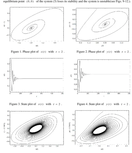
From the above analysis in section 2, If we choose 2 0, the equilibrium point ( 0 , 0 ) of the system (3) is asymptotically stable which proved by numerical simulations (see Figs. 1-4.).
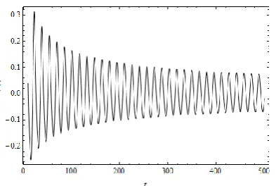
For convenient comparison, When 2 .3 3 4 9 6 0, a Hopf bifurcation occurs, namely, there are periodic
solutions bifurcating out from the equilibrium point ( 0 , 0 ) (see Figs. 5-8.). When 2 .5 >0 , the
equilibrium point ( 0 , 0 ) of the system (3) loses its stability and the system is unstable(see Figs. 9-12.).
Figure 1. Phase plot of x t( ) with 2 . Figure 2. Phase plot of y t( ) with 2 .
Figure 3. State plot of x t( ) with 2. Figure 4. State plot of y t( ) with 2 .
Figure 7. State plot of x t( ) with 2 .3 3 4 9 6. Figure 8. State plot of y t( ) with 2 .3 3 4 9 6.
Figure 9. Phase plot of x t( ) with 2 .5. Figure 10. Phase plot of y t( ) with 2 .5.
Figure 11. State plot of x t( ) with 2 .5. Figure 12. State plot of y t( ) with 2 .5.
V. CONCLUSIONS
Based on the original Rayleigh price model , a time-delayed feedback price model was studied by this paper.
Until now, there are few studies on price models with feedback delay and we provide an insight to unexplored aspects of them. By applying the control and bifurcation theory, We discussed the effect of the feedback delay
on the system. Moreover, we derived the conditions for the stability and the existence of Hopf bifurcation at the equilibrium of the system. By employing the theory of functional differential equations and the theory and applications of Hopf bifurcation, we obtained the the direction of Hopf bifurcation and the stability of
ACKNOWLEDGMENTS
The authors are grateful to the referees for their helpful comments and constructive suggestions.
REFERENCES
[1] Tang-Hong, L, and L. H. Zhou, “Hopf and Codimension Two Bifurcation in Price Rayleigh Equation with Two Time Delays,” Journal of Jilin University (Science Edition), vol. 50, no. 3, pp. 409-416, 2012.
[2] J. Li, W. Xu, W. Xie, Z. Ren, Research on nonlinear stochastic dynamical price model, Chaos Solitons & Fractals, vol. 37, no. 5, pp. 1391-1396, 2008.
[3] Tang-Hong, L, and L. H. Zhou, “Hopf and resonant codimension two bifurcation in price rayleigh equation with delays,” Journal of Northeast Normal University (Natrual Science Edition), vol. 44, no. 4, pp. 43–49,2012.
[4] W. Shuhe, Differential equation model and chaos, Journal of China Science and Technology University, pp. 312–324, 1999.
[5] Z. Xi-fan, C. Xia, and C. Yun-qing, “A qualitative analysis of price model in differential equations of price,” Journal of Shenyang Institute of Aeronautical Engineering, vol. 21, no. 1, pp. 83–86, 2004.
[6] T. Lv and Z. Liu, “Hopf bifurcation of price Rayleigh equation with time delay,” Journal of Jilin University, vol. 47, no. 3, pp.
441–448, 2009.
[7] B.D. Hassard, N.D. Kazarinoff, Y.H. Wan, Theory and Applications of Hopf Bifurcation, Cambridge University Press, Cambridge, 1981.
[8] Y. Kuang, Delay Differential Equations: With Applications in population Dynamics, Acdemic Press, New York, NY, USA, 1993.
[9] E. Beretta and Y. Kuang, “Geometric stability switch criteria in delay differential systems with delay dependent parameters,” SIAM Journal on Mathematical Analysis, vol. 33, no. 5, pp. 1144-1165, 2002.
[10]J. Hale, Theory of Functional Differential Equations, Springer, 1977.
[11]W. Yong and Z. Yanhui, “Stability and Hopf bifurcation of differential equation model of price with time delay,” Highlights of Sciencepaper Online, vol. 4, no. 1, 2011.
[12]D. Tao, X. Liao, T. Huang, Dynamics of a congestion control model in a wireless access network, Nonlinear Analysis: Real World Applications, vol. 14, no .1, pp. 671-683, 2013.
[13]D. Ding, J. Zhu, X.S. Luo, Delay induced Hopf bifurcation in a dual model of Internet congestion, Nonlinear Analysis: Real World Applications, vol. 10, no. 1, pp. 2873-2883, 2009.
[14]Y.G. Zheng, Z.H. Wang, Stability and Hopf bifurcation of a class of TCP/AQM networks, Nonlinear Analysis: Real World Applications, vol. 11, no. 3, pp. 1552-1559, 2010.
[15]Z.S. Cheng, J.D. Cao, Hybrid control of Hopf bifurcation in complex networks with delays, Neurocomputing, vol. 131, no. 131, pp. 164-170, 2014.
[16]D. Ding, X.Y. Zhang, et.al, Bifurcation control of complex networks model via PD controller, Neurocomputing ,vol. 175 (PA), pp. 1-9, 2016.
[17]D. Fan, J. Wei, Hopf bifurcation analysis in a tri-neuron network with time delay, Nonlinear Analysis: Real World Applications, vol. 9, no. 1, pp. 9-25,2008.