Nonparametric Bayesian Aggregation for Massive Data
Zuofeng Shang [email protected]
Department of Mathematical Sciences New Jersey Institute of Technology Newark, NJ 07102, USA
Botao Hao [email protected]
Department of Statistics Purdue University
West Lafayette, IN 47906, USA
Guang Cheng [email protected]
Department of Statistics Purdue University
West Lafayette, IN 47906, USA
Editor:Francis Bach
Abstract
We develop a set of scalable Bayesian inference procedures for a general class of nonparametric regression models. Specifically, nonparametric Bayesian inferences are separately performed on each subset randomly split from a massive dataset, and then the obtained local results are aggregated into global counterparts. This aggregation step is explicit without involving any additional computation cost. By a careful partition, we show that our aggregated inference results obtain an oracle rule in the sense that they are equivalent to those obtained directly from the entire data (which are computationally prohibitive). For example, an aggregated credible ball achieves desirable credibility level and also frequentist coverage while possessing the same radius as the oracle ball.
Keywords: Credible region, divide-and-conquer, Gaussian process prior, linear functional, nonparametric Bayesian inference
1. Introduction
With rapid development in modern technology, massive data sets are becoming more and more common. An important feature of massive data is their large volume which hinders applications of traditional statistical methods. For example, due to huge data amount and limited CPU memory, it is often impossible to process the entire data in a single machine. In the parallel computing environment, a common practice is to distribute massive data to multiple processors, and then aggregate local results in an efficient way. A series of frequentist methods such as Kleiner et al. (2011); McDonald et al. (2010); Zhang et al. (2015a); Zhao et al. (2016) have been proposed in this Divide-and-Conquer (D&C) framework.
In Bayesian community, there are quite a few computational or methodological works developed for massive data such as scalable algorithms for Bayesian variable selection Boom et al. (2015); Wang et al. (2014) and scalable posterior sampling in parametric models Wang and Dunson (2013); Wang et al. (2015). Theoretical guarantees of D&C methods have been
recently obtained in robust estimation Minsker et al. (2017), posterior interval estimation Srivastava et al. (2018), credible sets of signal in Gaussian white noise Szab´o and van Zanten (2019); Szabo and van Zanten (2018). Rather, the present paper puts focus on uncertainty quantification of the model parameter in general nonparametric regression, primarily in theoretical aspects. For instance, how to aggregate individual posterior means into a global one that maintains frequentist optimality? How to aggregate individual credible balls into a global one with a minimal possible radius? And how many divisions and what kind of priors should be chosen to guarantee Bayesian and frequentist validity of the aggregated ball? We attempt to address these questions in a univariate nonparametric regression setup.
Specifically, we develop a set of aggregation procedures in Bayesian nonparametric regression. As a first step, nonparametric Bayesian regression is separately fitted based on each subsample randomly split from a massive dataset. A variety of finite sample valid credible balls (credible intervals) for regression functions (their linear functionals Rivoirard et al. (2012), e.g., local values) are then constructed from each individual posterior distribution based on MCMC. In the second step, we aggregate these credible balls (credible intervals) into global counterparts analytically without involving any additional computation. For example, the center of an aggregated ball is obtained by weighted averaging Fourier coefficients of all individual (approximate) posterior modes, while the radius is given through an explicit formula on individual radii. A notable advantage of this distributed strategy is its dramatically faster computational speed, and this computational advantage becomes more obvious as data size grows.
Our aggregation procedures are proven to obtain an oracle rule in the sense that they are equivalent to those obtained directly from the entire data, i.e., called as oracle results which are computationally prohibitive in practice. For example, our aggregated posterior means are proven to achieve optimal estimation rate, and our aggregated credible ball achieves desirable credibility level and also frequentist coverage while possessing asymptotically the same radius as the oracle ball. These oracle results hold when the assigned Gaussian process priors in each subset are properly chosen and the number of subsets does not grow too fast. A fundamental theory underlying Bayesian aggregation is auniformversion of nonparametric Gaussian approximation theorem, also called as Bernstein-von Mises theorem. Developed based on our recent work Shang and Cheng (2017), this theory states that a sequence of individual posterior distributions converge to Gaussian processes uniformly over the number of subsets.
2. Nonparametric Bayesian Aggregation: An Illustration
In this section, we provide a concrete example to demonstrate the intuition of our non-parametric Bayesian aggregation procedure. Our example is based on the special uniform design and periodic Sobolev space which makes our aggregation procedure explicit and easy to understand. Section 2.1 describes our nonparametric Bayesian model, and Section 2.2 demonstrates our algorithm and its numeric performance. General aggregation procedures will be proposed in Sections 3 and 4 with asymptotic properties investigated as well.
2.1. Nonparametric Bayesian model
Suppose that we observe the dataZi= (Yi, Xi),i=1, . . . , N, generated from the following
Gaussian regression model with uniform design
Yi∣f, Xi∼N(f(Xi),1), X1, . . . , XN iid∼ U nif[0,1]. (1)
Randomly split{1,2, . . . , N} intossubsets I1, I2, . . . , Is with∣I1∣ = ⋯ = ∣Is∣ =n(so N =ns).
DenoteDj= {Zi∣i∈Ij}thej-th subsample forj=1, . . . , sandD= ∪sj=1Dj the entire sample.
Suppose that f belongs to anm-order periodic Sobolev spaceS0m[0,1] whereS0m[0,1]is the collection of all functions on [0,1] of the form
f(x) =√2∑∞
k=1
fkcos(2πkx) +
√
2∑∞
k=1
gksin(2πkx) (2)
with real coefficientsfk, gk satisfying
∞ ∑
k=1
(fk2+gk2)(2πk)2m< ∞. (3)
Here, m > 1/2 is a constant describing the smoothness of the functions. Wahba (1990) Wahba (1990) introduced a Gaussian process (GP) prior on f which has an interesting smoothing spline interpretation. Specifically, she assumed that the coefficientsfk, gk in (2)
are independent and normally distributed as follows:
fk, gk∼N(0,[(2πk)2m+β+nλ(2πk)2m]−1), k=1,2, . . . , (4)
where β>1 and λ≥0 are predecided constants. In particular, β represents the “relative smoothness” of the prior to the parameter space and λrepresents the amount of rescaling. Rescaling priors are also considered by Szab´o and van Zanten (2019); Szabo and van Zanten (2018) for constructing credible sets of signals in Gaussian white noise. It can be examined that if f satisfies (2) and (4), then f is a Gaussian process with mean zero and isotropic covariance function
K0(x, x′) =2
∞ ∑
k=1
cos(2πk(x−x′))
(2πk)2m+β+nλ(2πk)2m, x, x
′∈ [0,1]. (5)
provides a Bayesian interpretation for smoothing splines. Below we provide some details to justify this argument.
Let Πλ denote the probability distribution of f under (4). To derive the posterior
distribution, we need to find the “prior density” of f. Unlike the parametric settings where the prior densities are Radon-Nikodym (RN) derivatives w.r.t. Lebesgue measure, in the current infinite-dimensional setting it is impossible to do so since there is no Lebesgue measure on S0m[0,1] (see Hunt et al. (1992)). Instead, we need to characterize the prior density off as an RN derivative w.r.t. other kinds of measures such as Gaussian measure. Following Wahba Wahba (1990), Πλ and Π ≡Π0 (corresponding to λ=0) are equivalent
probability measures, and the RN derivative of Πλ w.r.t. Π is
dΠλ
dΠ (f) =
∞ ∏
k=1
(1+nλ(2πk)−β)−1×exp(−nλ 2
∞ ∑
k=1
(fk2+g2k)(2πk)2m)
= ∏∞
k=1
(1+nλ(2πk)−β)−1×exp(−nλ 2 ∫
1 0 f
(m)(x)2dx)
= ∏∞
k=1
(1+nλ(2πk)−β)−1×exp(−nλ
2 J(f)), (6)
where J(f) = ∫01f(m)(x)2dx. Note that∏k∞=1(1+nλ(2πk)−β)−1 converges thanks to β>1 so that (6) is a valid expression. (6) provides an expression for the prior density of f, which induces the following posterior distribution for f given subsamplej:
dP(f∣Dj) ∝ P(Dj∣f)dΠλ(f)
∝ exp⎛
⎝−
1 2i∑∈I
j
(Yi−f(Xi))2−
nλ
2 J(f)
⎞
⎠dΠ(f), j=1, . . . , s. (7)
Recall that Ij indexes the j-th subsample. The right hand-side of (7) corresponds to
penalized likelihood function `j(f) = −21n∑i∈Ij(Yi−f(Xi))
2−λ
2J(f) which has been well
studied in smoothing spline literature (Wahba (1990)). Theoretically, we recommend to choose λ≍N−2m2m+β which will be proven to yield optimal Bayesian inference; see Sections 3 and 4. The duality between the posterior and smoothing spline, i.e., (7), enables us to easily choose λfor practical use, e.g., GCV considered by Wahba (1990).
2.2. Nonparamtric Bayesian Aggregation
First of all, we calculate ˘fj,n=E{f∣Dj},j=1, . . . , s, the posterior means based on individual
posterior distributions (7). Then we construct a(1−α)-th credible ball centering at ˘fj,n with
radius rj,n(α). That is, rj,n(α) >0 such that P(f ∈S0m[0,1] ∶ ∥f−f˘j,n∥L2 ≤rj,n(α)∣Dj) =
1−α, where ∥ ⋅ ∥L2 is the usual L2-norm, i.e., ∥f∥L2 = √
∫01f(x)2dx. In practice, ˘fj,n
and rj,n(α) can be both estimated by the posterior samples. For instance, generate M
independent samples fj1, . . . , fjM from (7); estimate ˘fj,n by their average and estimate
rj,n(α) by the (1−α)-th percentile of ∥fjl−f˘j,n∥L2 for 1 ≤ l ≤ M. We postpone the
computational details of the sampling procedure to Section 8.5.
credible ball for f, denotedRN(α), is constructed with its center/radius obtained through
weighted averaging the individual centers/radii. Unlike simple averaging commonly used in
frequentist setting (see Zhang et al. (2015a)), our procedures for posterior mean aggregation and radius aggregation are weighted averaging with weightsws,N,λ,k defined in (10). These
weights are used to calibrate the prior effect such that the aggregation procedure can have satisfactory asymptotic property. The details of our procedure are demonstrated as follows:
1. Posterior mean aggregation. Forj-th subsample and k≥1, find
˘
fj,n,k=
√
2∫
1 0
˘
fj,n(x)cos(2πkx)dx, g˘j,n,k=
√
2∫
1 0
˘
fj,n(x)sin(2πkx)dx, (8)
where ˘fj,n is the posterior mean based on subsample j. Then we aggregate these
quantities through the following formulas:
˘
fN,λ,k= s
∑
j=1
˘
fj,n,k/s, ˘gN,λ,k= s
∑
j=1
˘
gj,n,k/s. (9)
In the end, we let
˘
fN,λ(x) =
∞ ∑
k=1
ws,N,λ,k{f˘N,λ,k
√
2 cos(2πkx) +g˘N,λ,k
√
2 sin(2πkx)}, (10)
wherews,N,λ,k= s(2πk)
2m+β+N(1+λ(2πk)2m)
(2πk)2m+β+N(1+λ(2πk)2m) fork≥1.
2. Posterior radius aggregation. Aggregate the radiirj,n(α)through the following formula:
rN(α) =
¿ Á Á Á ÀAN,s
⎛ ⎝ 1 s s ∑
j=1
rj,n(α)2
⎞
⎠+BN,s, (11)
where
AN,s=
√
C2/D2s−
4m+2β−1 2(2m+β),
BN,s= (2C1−2D1
√
C2/D2s−
1
2(2m+β))N− 2m+β−1
2m+β ,
Ck= ∫
∞
0 (1+ (2πx)
2m+ (2πx)2m+β)−kdx, k=1,2,
Dk= ∫
∞
0 (1+ (2πx)
2m)−kdx, k=1,2.
(12)
3. Aggregated credible ball:
RN(α) = {f∈Sm0 [0,1] ∶ ∥f −f˘N,λ∥L2 ≤rN(α)}. (13)
the aggregation steps involve proper weight averaging. Such algorithms are particularly useful to produce MCMC samples from the oracle posterior which can be used for various inferential purposes, e.g., estimation and testing. The present paper focuses on inferences, e.g., construction of credible balls, in a special class of nonparametric regression models, and has more extensive theoretical guarantees.
In practice, one can approximate the integral (8) through discretization; see Section 8.5. Theorem 3 will show that RN(α) given in (13) asymptotically covers 1−α mass of
the posterior based on the full data set and includes the true function with probability approaching one. More theoretical study on RN(α) such as its center and radius can be
found in Sections 4.2 and 4.3. Note that these sections present an aggregation procedure in a more general context, which covers (13) as a special case.
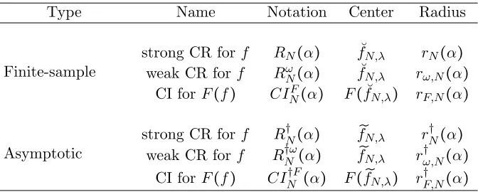
A toy simulation study was carried out to examine the proposed procedures (1)–(3). Specifically, we examine the computing time and coverage probability (CP) ofRN(α) for
various choices of s. The CP is defined as the relative frequency of the sets that cover the truth. We choosem=β =2 in our GP prior (4). Results are summarized in Figure 1. Plot (a) displays the true functionf0 under which data were generated. Plot (b) displays how the
CP varies as γ∶=log(s)/log(N). Plot (c) displays that the computing time decreases when
γ increases. There seems to be a transition for CP vs. γ, i.e., CP is uniformly close to one when 0≤γ <0.3 and approaches zero when γ>0.4. In conclusion, RN(α) possesses both
satisfactory frequentist coverage and computational efficiency whenγ ≈0.2. Other choices of γ either lower CP or slow down the computing. Thus, under a proper choice of s, our aggregation procedure can maintain good statistical properties and reduce computing burden at the same time. Careful readers may have noticed that the CP approaches one rather than the credibility level (1−α). This issue can be addressed by a modified aggregated set proposed in Section 4.4. More comprehensive simulation results are provided in Section 5 to examine various aggregation procedures such as the pointwise credible intervals.
0.0 0.2 0.4 0.6 0.8 1.0
0 2 4 6 8 10 12 14
(a)
x f0
(
x
)
0.0 0.1 0.2 0.3 0.4 0.5 0.6
0.0
0.2
0.4
0.6
0.8
1.0
(b)
γ
CP
0.0 0.1 0.2 0.3 0.4 0.5 0.6
10
20
30
40
50
60
(c)
γ
Time
Figure 1. Examination of our aggregation procedures (1)–(3). Results are based on N=1200observations
generated from (1) and a GP prior (4) with m = β = 2 and λ =N−2/3. (a) True regression function f0(x) =2.4β30,17(x) +1.6β3,11(x), whereβa,b is the probability density function forBeta(a, b). (b) Coverage
3. A Nonparametric Bayesian Framework Based on General Design and Space
In this section, we introduce a more general Bayesian nonparametric framework based on general design and function space under which the aggregation results will be obtained. Suppose that the data{Yi, Xi}Ni=1 follow a nonparametric regression model:
Yi∣f, Xiind.∼ N(f(Xi), σ2), X1, . . . , XN iid∼ π(x), (14)
where π(⋅)is a probability density on I= (0,1), andf belongs to anm-order Sobolev space
Sm(I):
Sm(I) = {f ∈L2(I)∣f(0), f(1), . . . , f(m−1)are abs. cont. andf(m)∈L2(I)}. (15)
In particular, S0m[0,1]is a proper subset of Sm(I). Throughout, we let m>1/2 such that
Sm(I) is a reproducing kernel Hilbert space (RKHS). For technical convenience, assume
σ2=1 and 0<infx∈Iπ(x) ≤supx∈Iπ(x) < ∞. When σ
2 is unknown, our approach can still
be applied with σ2 replaced by its consistent estimate.
For anyf, g∈Sm(I), defineV(f, g) =E{f(X)g(X)}andJ(f, g) = ∫01f(m)(x)g(m)(x)dx.
Following Shang et al. (2013), there exists a sequence of eigenfunctionsϕ1, ϕ2, . . .∈Sm(I)
and a sequence of eigenvalues 0=ρ1 =ρ2= ⋯ =ρm <ρm+1 ≤ρm+2 ≤ ⋯such that ρν ≍ν2m
and
V(ϕν, ϕµ) =δνµ, J(ϕν, ϕµ) =ρνδνµ, ν, µ≥1, (16)
whereδνµis the Kronecker’s delta.
We next place a prior distribution Πλ onf, where Πλ is a probability measure onSm(I)
and λ≥0 is a hyperparameter. Similar to Section 2, we will characterize Πλ through its
Radon-Nikodym (RN) derivative w.r.t. Π, with Π a pre-given probability measure Π on
Sm(I). Specifically, assume that the RN derivative of Πλ w.r.t. Π satisfies
dΠλ
dΠ (f) ∝exp(−
nλ
2 J(f)), (17)
whereJ(f) is defined in (3). Interestingly, it is possible to explicitly construct Πλ and Π
such that (17) holds. To see this, let
Gλ(⋅) =
∞ ∑
ν=m+1
wνϕν(⋅), (18)
wherewν’s are independent of the observations satisfyingwν ∼N(0,1/(ρν1+β/(2m)+nλρν)), ν>
m. Let G(⋅) =Gλ=0(⋅). Suppose Πλ and Π are probability measures induced byGλ and G,
i.e., Πλ(S) =P(Gλ∈S) and Π(S) =P(G∈S) for any measurableS⊆Sm(I). It follows by
H´ajek’s lemma (see Shang and Cheng (2017)) that (17) holds. In (18), λ≥0 andβ>1 are both hyper-parameters characterizing the smoothness of the prior. It is easy to check that the sample path of Gλ belongs to Sm(I) for any β>1 almost surely. As demonstrated in a
4. Main Results
In this section, we present a series of main results that are built upon a uniform Gaussian approximation theorem (Section 4.1). Three classes of aggregation procedures are then proposed: aggregated credible balls in both strong and weak topology, and aggregated credible intervals for linear functionals. These results can be classified into two types: finite
sampleconstruction (Sections 4.3, 4.4 and 4.5) andasymptotic construction (Section 4.6).
The former construction is often time-consuming since its radius (interval length) is obtained throughs posterior sampling, while the latter employs a large-sample limit of the radius given by an explicit formula. The computational gain will be illustrated by the simulations in Section 5. Similar to Section 2, let I1, I2, . . . , Is be a random partition of {1,2, . . . , N}
such that∪sj=1Ij = {1,2, . . . , N} with∣Ij∣ =nforj=1, . . . , sand N =ns. 4.1. A Uniform Gaussian Approximation Theorem
A fundamental theory underlying Bayesian aggregation is developed in this section. It is a
uniformversion of Gaussian approximation theorem that characterizes the limit shapes of a
sequence of individual posterior distributions. This uniform validity holds if the number of posterior distributions does not grow too fast. Also, Bayesian aggregation procedures possess frequentist validity ifλis chosen properly.
Similar to (7), we note that each sub-posterior distribution can be written as
dP(f∣Dj) ∝exp(n`jn(f))dΠ(f),
where`jn(f) =n−1∑i∈Ij(Yi−f(Xi))
2− (λ/2)J(f). Define
̂
fj,n=arg max f∈Sm( I)
`jn(f), j=1, . . . , s. (19)
Suppose that f̂j,n admits the following Fourier expansion:
̂ fj,n(⋅) =
∞ ∑
ν=1
̂
fν(j)ϕν(⋅), 1≤j≤s. (20)
Define h=λ1/(2m) with h∗∶=N−2m1+β. We remark that h∗ is an optimal choice for our aggregation procedure as will be shown later.
Theorem 1 (Uniform Gaussian Approximation) Suppose thatf0 admits a Fourier expansion
f0(⋅) = ∑∞ν=1fν0ϕν(⋅) which further satisfies
Condition (S)∶ ∑∞
ν=1
∣fν0∣2ρ1+
β−1 2m
ν < ∞
If the following holds
m>1+
√
3
2 ≈1.866,1<β<2m+ 1
2m−1, s=o(N
β−1
2m+β) and h≍h∗, (21)
then we have as N → ∞,
sup
S∈S
max
1≤j≤s∣P(S∣Dj) −P0j(S)∣ =OPf0 ( √
sN−
4m2+2mβ−10m+1
where S is the Borel σ-algebra on Sm(I) with respect toΠ, andP0j’s are GPs defined by
P0j(S) = ∫S
exp(−n2∥f− ̂fj,n∥2)dΠ(f)
∫Sm(
I)exp(−
n
2∥f− ̂fj,n∥2)dΠ(f)
, S∈ S. (23)
Proof of Theorem 1 is rooted in Shang and Cheng (2017) who essentially considered s=1. Substantial efforts have been made here to quantify a range of partition size s such that local posteriors can be uniformly approximated by GPs. The explicit structure of the GPs provides a guideline for our aggregation procedures which will be introduced in subsequent sections. It should be emphasized that our aggregation of GPs is weighted-averaging which is different from product-based ones such as Cao and Fleet (2014).
Condition (S) amounts to requiring known regularity of the truth f0∈Sm+
β−1
2 (I). This
can be seen from the inequality ∑∞ν=1∣fν0∣2ν2m+β−1 < ∞ since ρν ≍ ν2m. This condition
essentially means thatf0 has derivatives up to orderm+β−21 (when this order is
integer-valued). Combined with (21) this means that the regularity off0 belongs to(m,2m+41m−1),
i.e., the truth function is jointly confined by both functional space and the prior. The∥⋅∥-norm used in (23) is defined as follows. For anyg,̃g∈Sm(I), define
⟨g,̃g⟩ =V(g,g̃) +λJ(g,̃g) (24)
and its squared norm∥g∥2= ⟨g, g⟩. Clearly,⟨⋅,⋅⟩ is a valid inner product onSm(I). Remark 1 We remark that (21) can be replaced by a more general rate condition:
nh2m+1≥1, an=O(̃rn), bn≤1, r2nbn≤ ̃rn2, ñr2nbn=o(1),
where rn = (nh)−1/2 +hm,̃rn = (nh/log 2s)−1/2 +hm+
β−1
2 , an = n−1/2h− 6m−1
4m rnlogN, bn =
n−1/2h−6m4m−1(logN)3/2. Here, we provide a technical explanation for the terms rn,̃rn, an, bn.
Specifically,rn can be viewed as the rate of convergence of local ordinary penalized MLE (19),
̃
rn can be viewed as the posterior contraction rate of the local Bayesian mode, an, bnare error
bounds of the higher-order remainders in the Taylor expansions of the individual penalized
likelihood functions. Uniform Gaussian approximation for generalh (not necessarily h≍h∗)
can be established under such condition.
Theorem 3.5 in Shang and Cheng (2017) shows that P0j (conditional on Dj) is induced
by a Gaussian process, denoted as Wj, in the sense that P0j(S) =P(Wj ∈S∣Dj) for any
S∈ S. Define
τν2=ρ1+
β 2m
ν , ν≥1. (25)
Then we have
Wj(⋅) = ∞ ∑
ν=1
(an,νf̂ν(j)+bn,ντνvν)ϕν(⋅), j=1,2, . . . , s,
where an,ν =n(1+λρν)(τν2+n(1+λρν))−1,bn,ν = (τν2+n(1+λρν))−1/2 andvν ∼N(0, τν−2).
For convenience, define the mean functions of Wj as
̃ fj,n(⋅) ∶=
∞ ∑
ν=1
such that we can re-express Wj as
Wj= ̃fj,n+Wn, j=1, . . . , s,
where Wn(⋅) ∶= ∑∞ν=1bn,ντνvνϕν(⋅) is a zero-mean GP. Note that the posterior modef̃j,n is
very close tof̂j,n since∥ ̃fj,n− ̂fj,n∥ =oPf0(1)uniformly for 1≤j≤s; see the proof of Theorem 3. The above characterization of Wj is useful for the subsequent Bayesian aggregation procedures.
4.2. Aggregated posterior means
In this section, we propose a method to aggregate the posterior means ˘fj,n ∶=E{f∣Dj},
for j = 1, . . . , s. The aggregated mean function, denoted as ˘fN,λ(⋅), can be viewed as a
nonparametric Bayesian estimate of f, and will be used to construct aggregated credible balls/intervals to be introduced later.
Our aggregation procedure is
˘
fN,λ(⋅) =
∞ ∑
ν=1
aN,ν
an,ν
V⎛
⎝
1
s
s
∑
j=1
˘
fj,n, ϕν
⎞
⎠ϕν(⋅). (27)
Note that when the model is Gaussian and f ∈ S0m(0,1), (27) becomes (10). Next we will show that the aggregation procedure (27) yields minimax optimality in the following theorem.
Theorem 2 Under conditions of Theorem 1, the following result holds:
max
1≤j≤s∥
˘
fj,n− ̃fj,n∥ =OPf0(̃rn
√
sN−
4m2+2mβ−10m+1
4m(2m+β) (logN)52), (28)
If, in addition, 3/2<β <2m+1/(2m) −3/2 and ssatisfies
s=o(N
4m2+2mβ−11m+1
8m(2m+β) (logN)−32), (29)
then it holds that
∥f˘N,λ−f0∥2=OP f0(N
−2m+β−1
2(2m+β)), (30)
where ∥f∥2=
√
V(f) denotes the V-norm.
According to van der Vaart et al. (2008b), the rate in (30) is minimax optimal given Condition (S).
4.3. Aggregated credible region in strong topology
property is achieved as long as s is not diverging fast and the assigned GP prior in each subset is chosen by setting h ≍ h∗, i.e., λ ≍ N−2m/(2m+β). The conservative frequentist coverage can be improved to the nominal level if we use a weaker norm in defining credible region; see Section 4.4.
Based on each subset Dj, the individual credible ball is constructed as follows:
Rj,n(α) = {f∈Sm(I) ∶ ∥f−f˘j,n∥2≤rj,n(α)}.
The credible ball centers around the posterior mean ˘fj,n, while its radius rj,n(α) is directly
sampled from MCMC such thatP(Rj,n(α)∣Dj) =1−α for anyα∈ (0,1). We will construct
an “aggregated” region centering at ˘fN,λwith radius explicitly constructed as follows:
rN(α) =
¿ Á Á Á
À 1
N ⎡⎢ ⎢⎢ ⎢⎣ζ1,N+
¿ Á Á Àζ2,N
ζ2,n
⎛ ⎝ n s
s
∑
j=1
r2
j,n(α) −ζ1,n
⎞ ⎠ ⎤⎥ ⎥⎥
⎥⎦, (31)
where
ζk,n=
∞ ∑
ν=1
( n
τ2
ν +n(1+λρν)) k
fork=1,2.
The final aggregated credible region is obtained as
RN(α) ∶= {f ∈Sm(I) ∶ ∥f−f˘N,λ∥2≤rN(α)}. (32)
Our theorem below confirms thatRN(α)indeed possesses (asymptotic) posterior mass
(1−α), and more importantly, proves that it covers the true functionf0 with probability
tending to one.
Theorem 3 Suppose thatf0 satisfies Condition (S),m>1+
√
3
2 ,3/2<β<2m+1/(2m)−3/2,
s=o(N
β−1
2m+β), (29) andh≍h∗. Then for any α∈ (0,1), P(R
N(α)∣D) =1−α+oPf0(1) and
limn→∞Pf0(f0∈RN(α)) =1.
From the proof of Theorem 3, we point out that when s=1, the posterior mass of the aggregated credible region is exactly 1−α, consistent with Shang and Cheng (2017). This remark also applies to other aggregated procedures to be presented later.
Remark 2 When h≍h∗, the radius of the aggregated ball rN(α) ≍N−
2m+β−1
2(2m+β) according to the discussions in Section 4.6. This is the optimal rate at which a posterior ball contracts based on the entire sample; see van der Vaart et al. (2008b).
4.4. Aggregated credible region in weak topology
In this section, we invoke a weaker norm (than that used in Section 4.3) to construct an aggregated credible region. Under this new norm (inspired by Castillo et al. (2013, 2014)), it is proven that the frequentist coverageexactly matches with the asymptotic credibility level. The requirement onsand h in this section remains the same as Section 4.3.
We define a weaker norm than∥ ⋅ ∥2, denoted∥ ⋅ ∥ω. For any f ∈Sm(I) withf = ∑νfνϕν,
all ν≥1, we have ∥f∥ω≤ ∥f∥2. Under the new∥ ⋅ ∥ω-norm, each individual (1−α) credible
region is constructed as
Rωj,n(α) = {f∈Sm(I) ∶ ∥f−f˘j,n∥ω≤rω,j,n(α)},
whererω,j,n(α)is directly obtained from posterior sampling such thatP(Rj,nω (α)∣Dj) =1−α.
Under ∥ ⋅ ∥ω-norm, the aggregated credible region is constructed as:
RωN(α) ∶= {f ∈Sm(I) ∶ ∥f−f˘N,λ∥ω≤rω,N(α)}, (33)
where the radius is given as
rω,N(α) =
¿ Á Á
À1
s2
s
∑
j=1
r2
ω,j,n(α). (34)
Interestingly, Section 4.6 illustrates that the aggregated radiusrω,N(α) contracts at root-N
rate.
Our theorem below shows that the frequentist covergage of RωN(α) exactly matches with the asymptotic posterior mass, both of which achieve the nominal level(1−α).
Theorem 4 Suppose that f0 satisfies Condition (S), m > 1+
√
3/2, 2 ≤ β < (2m2m−1)2,
s = o(N
β−1
2m+β), s = o(N
4m2+2mβ−12m+1
8m(2m+β) (logN)−23), and h ≍ h∗. Then for any α ∈ (0,1),
P(RNω(α)∣D) =1−α+oPf0(1) and limn→∞Pf0(f0∈R
ω
N(α)) =1−α.
4.5. Aggregated credible interval for linear functional
In this section, we construct aggregated credible intervals for a class of linear functionals of f, denoted asF(f). Examples include the evaluation functional, i.e., F(f) =f(x), and integral functional, i.e., F(f) = ∫01f(x)dx. Specifically, the interval is centered atF(f˘N,λ)
with an length aggregated throughslengths obtained from posterior sampling. Posterior and frequentist coverage properties of this aggregated interval depends on the functional form F(⋅). Again, our theory holds whensis mildly diverging and h≍h∗.
Let F∶Sm(I) ↦Rbe a linear Π-measurable functional satisfying the following Condition
(F): supν≥1∣F(ϕν)∣ < ∞, and there exist constants κ >0 and r ∈ [0,1] such that for any
f ∈Sm(I),
∣F(f)∣ ≤κh−r/2∥f∥. (35)
It follows by Shang and Cheng (2017) that the evaluation functional satisfies Condition (F) withr=1 and the integral functional satisfies Condition (F) withr=0.
Based on each Dj, we obtain from posterior samples the following (1−α) credible
interval:
CIj,nF (α) ∶= {f ∈Sm(I) ∶ ∣F(f) −F(f˘j,n)∣ ≤rF,j,n(α)},
where rF,j,n(α) is a radius such that P(CIj,nF (α)∣Dj) = 1−α. The aggregated credible
interval is constructed as
where
rF,N(α) =
θ1,N
θ1,n
¿ Á Á
À1
s
s
∑
j=1
rF,j,n(α)2 and θk,n2 =
∞ ∑
ν=1
F(ϕν)2
(τ2
ν +n(1+λρν))k
fork=1,2. (37)
The shrinking rate of ¯rF,N(α)depends on the functional form F; see Section 4.6.
Our theorem below investigates the asymptotic properties of CIFN(α) in terms of both posterior and frequentist coverage.
Theorem 5 Suppose that f0 = ∑∞ν=1fν0ϕν satisfies Condition (S′): ∑∞ν=1∣fν0∣2ν2m+β < ∞,
Ef0{
4∣X} ≤M
4 a.s. for some constant M4 > 0, Nkθ2k,N ≳ h−r for k = 1,2, m > 1+
√
3 2 ,
2≤β <(2m2m−1)2, s=o(N
β−1
2m+β), s=o(N
4m2+2mβ−12m+1
8m(2m+β) (logN)−32), (29) and h≍h∗. Then for any α∈ (0,1), P(CINF(α)∣D) =1−α+oPf0(1), and lim infN→∞Pf0(f0 ∈CI
F
N(α)) ≥1−α
given that Condition (F) holds. Moreover, if 0< ∑∞ν=1F(ϕν)2< ∞, then limN→∞Pf0(f0 ∈
CINF(α)) =1−α.
Note that Condition (S′) is slightly stronger than Condition (S) required in Theorem 1. Indeed, this condition essentially means that f0 has derivatives up to orderm+β2 (when
this order is integer-valued). Hence, Theorem 5 requires a more smooth true functionf0.
It was shown in Shang and Cheng (2017) that the integral functionalFx(f) ∶= ∫0xf(z)dz
for anyx∈ [0,1]satisfies (35) withr=0 and 0< ∑∞ν=1Fx(ϕν)2< ∞. Therefore, the(1−α)-th
credible interval of Fx(f) achieves exactly (1−α) frequentist coverage, while that for the
evaluation functional is more conservative. These theoretical findings will be empirically verified in Section 5 .
4.6. Asymptotic aggregated inference
In practice, the centers ˘fN,λ,F(f˘N,λ) and the radii rj,n(α),rω,j,n(α),rF,j,n(α)in Sections
4.3 – 4.5 are directly obtained from posterior samples. Sometimes posterior sampling is time consuming and inefficient, particularly as s→ ∞. This computational consideration motivates us to propose anasymptotic approach in which one replaces the above centers/radii by their large sample limits. Our new asymptotic inference procedures dramatically improve the computing speed, as displayed in simulations; see Section 5.
Define
̃ fN,λ(⋅) =
∞ ∑
ν=1
aN,ν
an,ν
V⎛
⎝
1
s
s
∑
j=1
̃
fj,n, ϕν
⎞
⎠ϕν(⋅). (38)
Clearly,f̃N,λ is a counterpart of ˘fN,λ (27) with ˘fj,n therein replaced byf̃j,n. By a careful
examination of the proofs of Theorems 3 – 5, it can be shown that the following limits hold:
∥f˘N,λ− ̃fN,λ∥ = oP f0(N
−1/2h−1/4),
max
1≤j≤s∣
nrj,n2 (α) −ζ1,n
√
2ζ2,n
−zα∣ = oPf0(1),
max
1≤j≤s∣
√
nrω,j,n(α) −√cα∣ = oPf0(1),
max
where zα=Φ−1(1−α) with Φ(⋅) being the c.d.f. of standard normal random variable, and
cα>0 satisfiesP(∑∞ν=1dνην2≤cα) =1−αwithην being independent standard normal random
variables.
It yields from (39) that the following approximation relationships hold uniformly for 1≤j≤s:
rj,n(α) ≈
¿ Á Á Àζ1,n+
√
2ζ2,nzα
n , rω,j,n(α) ≈
√c
α
n and rF,j,n(α) ≈θ1,nzα/2,
which further implies (by the aggregation formulae (31), (34) and (37))
rN(α) ≈rN†(α) ∶=
¿ Á Á Àζ1,N+
√
2ζ2,Nzα
N ,
rω,N(α) ≈rω,N† (α) ∶=
√c
α
N,
rF,N(α) ≈r†F,N(α) ∶=θ1,Nzα/2.
(40)
Thus, we have the followingasymptoticcounterparts of RN(α),RNω(α) andCINF(α):
R†N(α) ∶= {f ∈Sm(I) ∶ ∥f− ̃fN,λ∥2≤r†N(α)}, (41)
R†Nω(α) ∶= {f ∈Sm(I) ∶ ∥f− ̃fN,λ∥ω≤r†ω,N(α)}, (42)
CIN†F(α) ∶= {f ∈Sm(I) ∶ ∣F(f) −F( ̃fN,λ)∣ ≤rF,N† (α)}. (43)
Our theorem below shows that the posterior coverage and frequentist coverage of the above computationally efficient alternatives remain the same as those for RN(α),RωN(α)
and CINF(α) under the same set of conditions.
Theorem 6 Suppose that all assumptions in Theorems 3 – 5 hold. Then for anyα∈ (0,1), RN† (α),R†Nω(α) and CIN†F(α) possess exactly the same posterior and frequentist properties as RN(α),RωN(α) and CINF(α), respectively.
As a byproduct, (40) implies the contraction rate of each aggregated credible ball/interval in Sections 4.3 – 4.6. It is easy to see that rω,N(α) ≍N−1/2. As for rF,N(α), it depends
on the functional formF. For example, when F is an evaluation functional, it holds that
θ21,N ≍ (N h)−1, leading to N− 2m+β−1
2(2m+β) when h ≍ h∗; when F is an integral functional, we have rF,N(α) ≍N−1/2 since θ12,N ≍N−1. As for rN(α), it can be shown by a simple fact
ζ1,N, ζ2,N≍h−1 thatrN(α) ≍ (N h)−1/2≍N−
2m+β−1
2(2m+β) whenh≍h∗. This contraction rate turns out to be optimal based on the entire sample; see van der Vaart et al. (2008b). However, if we choose hin the scale of subsample size n, e.g., h≍n−2m1+β, similar arguments show that
rN(α) ≍N−
2m+β−1 2(2m+β)s−
1
2(2m+β). Hence, such a region contracts faster than the optimal rate, which results in unsatisfactory frequentist coverage.
Table 1. Summary of Aggregated (1−α) Credible Regions/Intervals
Type Name Notation Center Radius
Finite-sample
strong CR for f RN(α) f˘N,λ rN(α)
weak CR forf RωN(α) f˘N,λ rω,N(α)
CI forF(f) CINF(α) F(f˘N,λ) rF,N(α)
Asymptotic
strong CR for f R†N(α) f̃N,λ r†N(α)
weak CR forf R†Nω(α) f̃N,λ r†ω,N(α)
CI forF(f) CIN†F(α) F( ̃fN,λ) r†F,N(α)
5. Simulation Study
In this section, statistical properties of the proposed aggregated procedures are examined using a simulation study. We generated samples from the following model
Yij =f0(Xij) +ij, i=1,2, . . . , n, j =1,2, . . . , s, (44)
where Xijiid∼ U nif[0,1],ij iid∼ N(0,1), and ij are independent ofXij. The true regression
function was chosen to be f0(x) =2.4β30,17(x) +1.6β3,11(x), where βa,b is the probability
density function for Beta(a, b).
Consider GP prior f ∼ ∑nν=1wνϕν, where wν are defined in (18). The proposed Bayesian
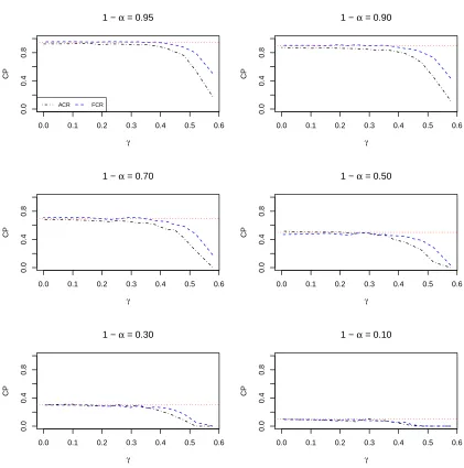
procedures were examined. Specifically, we computed the frequentist coverage proportions (CP) of the credible regions (32), (33), (41), (42), and credible intervals (36), (43). In particular, (32), (33) and (36) were constructed based on posterior samples, as described in Sections 4.2–4.5; whereas (41), (42) and (43) were constructed based on asymptotic theory developed in Section 4.6. To ease presentation, we call (32) and (33) as finite-sample credible regions (FCR), and call (41) and (42) as asymptotic credible regions (ACR).
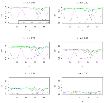
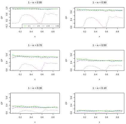
The calculation of CP was based on 500 independent experiments. Specifically, the CP is the proportion of the credible regions/intervals containing f0/F(f0) (for a linear functional
F). Two types of F were considered: (1) the evaluation functional Fx(f) =f(x) for any
x∈ [0,1], and (2) the integral functional Fx(f) = ∫0xf(z)dz for any x∈ [0,1]. In both cases,
we considerFx withx being 15 evenly spaced points in [0.05,0.95]. To make the study more
complete, a set of credibility levels were examined, i.e., 1−α=0.1,0.3,0.5,0.7,0.9,0.95. In each experiment,N =1200 independent samples were generated from the model (44). For ACR and FCR, we chose the number of divisionss=1,2,3,4,5,6,8,10,12,15,20,24,30,40,60. Define γ=logs/logN. Note that s=1 (equivalently,γ=0) means “no division.”
0.0 0.1 0.2 0.3 0.4 0.5 0.6
0.0
0.4
0.8
1 − α = 0.95
γ
CP
ACR FCR
0.0 0.1 0.2 0.3 0.4 0.5 0.6
0.0
0.4
0.8
1 − α = 0.90
γ
CP
0.0 0.1 0.2 0.3 0.4 0.5 0.6
0.0
0.4
0.8
1 − α = 0.70
γ
CP
0.0 0.1 0.2 0.3 0.4 0.5 0.6
0.0
0.4
0.8
1 − α = 0.50
γ
CP
0.0 0.1 0.2 0.3 0.4 0.5 0.6
0.0
0.4
0.8
1 − α = 0.30
γ
CP
0.0 0.1 0.2 0.3 0.4 0.5 0.6
0.0
0.4
0.8
1 − α = 0.10
γ
CP
Figure 2. CP of ACR and FCR based on strong topology. Dotted red lines indicate credibility levels.
topology tends to be more “conservative.” Figure 3 demonstrates the results for FCR and ACR based on weak topology, i.e., (33) and (42). We observe that the CP of both ACR and FCR approaches the desired credibility levels whenγ ≤0.3, but quickly drops to zero when
γ becomes large. This observation also supports our theory that the use of weak topology leads to a more satisfactory frequentist coverage.
0.0 0.1 0.2 0.3 0.4 0.5 0.6
0.0
0.4
0.8
1 − α = 0.95
γ
CP
ACR FCR
0.0 0.1 0.2 0.3 0.4 0.5 0.6
0.0
0.4
0.8
1 − α = 0.90
γ
CP
0.0 0.1 0.2 0.3 0.4 0.5 0.6
0.0
0.4
0.8
1 − α = 0.70
γ
CP
0.0 0.1 0.2 0.3 0.4 0.5 0.6
0.0
0.4
0.8
1 − α = 0.50
γ
CP
0.0 0.1 0.2 0.3 0.4 0.5 0.6
0.0
0.4
0.8
1 − α = 0.30
γ
CP
0.0 0.1 0.2 0.3 0.4 0.5 0.6
0.0
0.4
0.8
1 − α = 0.10
γ
CP
above the credibility levels except for the points where the true function f0 has peaks; see
(a) of Figure 1. The observation that the CP stays above(1−α) coincides with our theory that the credible interval of the evaluation functional is conservative. On the other hand, it can be seen that whens=60, the CP of the credible intervals for the integral functional becomes far below the credibility levels at mostx. However, whens=1,6,15, the CP is close to the credibility levels at allx. This finding coincides with our theory that the the credible interval of the integral functional achieves exactly (1−α) frequentist coverage. The above results also support our claim thatscannot grow too fast for guaranteeing frequency validity. Credible intervals based on asymptotic theory, i.e., (43), were summarized in Figures 11 and 12 of the supplement document Shang and Cheng. Interpretations of these results are similar to those based on finite posterior samples.
The supplement document Shang and Cheng also includes Figures 13 – 16 which demonstrate how the radii/lengths of the aggregated credible regions/intervals change along with γ, the size of the subsample. It can be observed that whenγ ≤0.3, indicating that the full sample is divided into at most twelve subsamples, the radii of the aggregated regions/intervals are almost identical to the radii of the regions/intervals directly constructed from the full sample, i.e., γ =0. This means that our aggregated procedures, based on a suitable amount of divisions, indeed mimic the oracle procedures. However, whenγ increases to 0.6, the distinctions between the the aggregated and oracle procedures quickly become obvious.
We also repeated the above study for N =1800 and 2400. The plots corresponding to these studies are given in supplement document; see Section S.8.6 of Shang and Cheng. The interpretations of these additional results are similar as above.
To the end of this section, computing efficiency is investigated. Figure 6 displays the results based on a single experiment for various choices of N. Specifically, we look at the value of the quantity ρ=1− (T/T0) versus a collection of γ’s for FCR and ACR, where
T0 (T) is the computing time without using D&C (based on D&C). We observe that T is
substantially smaller than T0, and this computation efficiency (as reflected by the value of
ρ) becomes more obvious as γ grows for each fixed N. This can also be seen asN grows for each fixed γ. However, this reduction in computing time does not affect the performances of the aggregated credible regions when 0≤γ ≤0.3, as demonstrated in Figures 2, 3, 13–16.
6. Real Data Analysis
In this section, we apply our methods to Million Song Data (MSD) and Flight Delay Data (FDD).
6.1. Million Song Data
As a real application, we apply our aggregation procedure to analyze MSD. The MSD is a perfect example of large dataset, a freely-available collection of audio features and metadata for a million contemporary popular music tracks. Each observation is a song track released between the year 1922 and 2011. The response variable Yi is the year when
the song was released and the covariate Xi is the timbre average of the song. The main
0.2 0.4 0.6 0.8
−0.2
0.2
0.6
1.0
1 − α = 0.95
x
CP
s=1 s=6 s=15 s=60
0.2 0.4 0.6 0.8
0.0
0.4
0.8
1 − α = 0.90
x
CP
0.2 0.4 0.6 0.8
0.0
0.4
0.8
1 − α = 0.70
x
CP
0.2 0.4 0.6 0.8
0.0
0.4
0.8
1 − α = 0.50
x
CP
0.2 0.4 0.6 0.8
0.0
0.4
0.8
1 − α = 0.30
x
CP
0.2 0.4 0.6 0.8
0.0
0.4
0.8
1 − α = 0.10
x
CP
Figure 4. CP of Fx(f) =f(x) against x based on posterior samples of f. Dotted red lines indicate
0.2 0.4 0.6 0.8
−0.2
0.2
0.6
1.0
1 − α = 0.95
x
CP
s=1 s=6 s=15 s=60
0.2 0.4 0.6 0.8
0.0
0.4
0.8
1 − α = 0.90
x
CP
0.2 0.4 0.6 0.8
0.0
0.4
0.8
1 − α = 0.70
x
CP
0.2 0.4 0.6 0.8
0.0
0.4
0.8
1 − α = 0.50
x
CP
0.2 0.4 0.6 0.8
0.0
0.4
0.8
1 − α = 0.30
x
CP
0.2 0.4 0.6 0.8
0.0
0.4
0.8
1 − α = 0.10
x
CP
Figure 5. CP ofFx(f) = ∫
x
0 f(z)dzagainstxbased on posterior samples off. Dotted red lines indicate
0.1 0.2 0.3 0.4 0.5
0.6
0.7
0.8
0.9
1.0
N=1200
γ
ρ
ACR FCR
0.1 0.2 0.3 0.4 0.5
0.6
0.7
0.8
0.9
1.0
N=4800
γ
ρ
ACR FCR
0.1 0.2 0.3 0.4 0.5
0.6
0.7
0.8
0.9
1.0
N=9600
γ
ρ
ACR FCR
Figure 6. ρversusγ based on FCR and ACR for single experiment.
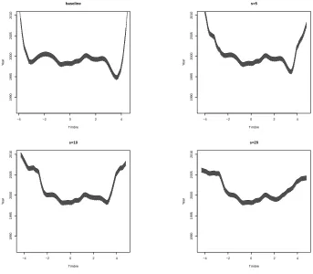
predict production year based on song timbre. Due to enormous sample size, processing the entire data is infeasible. In frequentist setting, a distributed kernel ridge regression method was proposed by Zhang et al. (2015a,b) for estimation purposes (without quantifying uncertainty).
In the Bayesian setup, we applied our aggregation procedure to construct 95% credible sets for f based on a subset ofN =10,000 songs released from the year 1996 to 2010. We randomly split the observations tos=5,10,20 subsets. We also compared our results with the baseline method in which all ten thousand observations were used. Credible sets are displayed as gray areas in Figure 7. We find that the shapes of all credible sets are overall the same when the timbre ranges from -4 to 4, e.g., all display a W-shape, although the results are a bit sensitive near the endpoints. Therefore, the overall pattern of the sets appears to be insensitive to the above selections ofs.
6.2. Flight Delay Data
−4 −2 0 2 4
1990
1995
2000
2005
2010
baseline
Timbre
Y
ear
−4 −2 0 2 4
1990
1995
2000
2005
2010
s=5
Timbre
Y
ear
−4 −2 0 2 4
1990
1995
2000
2005
2010
s=10
Timbre
Y
ear
−4 −2 0 2 4
1990
1995
2000
2005
2010
s=20
Timbre
Y
ear
Figure 7. 95% Credible sets (grey areas) forf based on a subset of 10,000 samples in Million Song Data.
The first plot refers to the baseline method where the whole samples were used. The rest three plots refer to the aggregation procedure which was applied to 5, 10, 20 random splits.
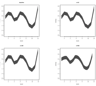
impact on the flight delay. We considered the relationship (denotedf) between month and the length of the flight delay, i.e., length of flight delay=f(month)+error. Negative length of delay implies that the flight arrived earlier. We applied the same Bayesian aggregation procedure as described in MSD to a randomly selected subset ofN =10,000 flight information in the year 2007. We randomly split the observations to s=10,100,500 subsamples, based on which the aggregated credible sets for f were constructed. We also compared the results with the baseline where all the ten thousand samples were used. Credible sets are displayed as gray areas in Figure 8. Again, the shapes of the four credible sets appear to be almost the same for alls.
6.3. Computation Efficiency
2 4 6 8 10 12
−10
−5
0
5
10
15
20
baseline
Month
ArrDela
y
2 4 6 8 10 12
−10
−5
0
5
10
15
20
s=10
Month
ArrDela
y
2 4 6 8 10 12
−10
−5
0
5
10
15
20
s=100
Month
ArrDela
y
2 4 6 8 10 12
−10
−5
0
5
10
15
20
s=500
Month
ArrDela
y
Figure 8. 95% Credible sets (grey areas) forf based on a subset of 10,000 samples in Flight Delay Data.
The first plot refers to the baseline method where the whole samples were used. The rest three plots refer to the aggregation procedure which was applied to 10, 100, 500 random splits.
7. Conclusions
This paper proposes algorithms for aggregating individual posterior results such as modes, balls, intervals, into their global counterparts. The algorithms are easy-to-implement which are particularly useful in big data scenarios. We also experimented the proposed algorithms through simulated and real data sets. A notable contribution of this article is to provide rigorously justified theoretical guarantees. The major tool for proving our theoretical results is a uniform Gaussian approximation theorem which shows that the individual posterior distributions converge uniformly to Gaussian processes provided that the number of subsets is not too large.
Acknowledgments
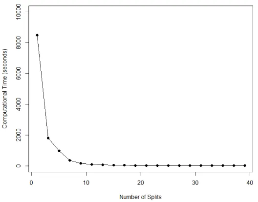
Figure 9. Computational time of aggregation procedures for MSD.
8. APPENDIX
This appendix section contains the proofs of the main results. Section 8.1 contains proof of Theorem 1 and relevant preliminary results. Section 8.2 includes the proof of Theorem 2. Sections 8.3 and 4.4 includes the proofs of Theorems 3 and 4, i.e., coverage properties of the credible sets based on strong and weak topology respectively.
All proofs crucially depend on an eigensystem designed for simultaneous diagonalization of the two bilinear functionalsU, V induced from likelihood and prior, respectively. In fact,
(ϕν, ρν) is a solution of the following ordinary differential system (whose existence and
uniqueness is guaranteed by Birkhoff (1908)):
(−1)mϕν(2m)(⋅) =ρνπ(⋅)ϕν(⋅),
ϕ(νj)(0) =ϕ(νj)(1) =0, j =m, m+1, . . . ,2m−1, (1)
Properties of this eigen-system are summarized in Proposition 1, whose proof can be found in (Shang et al., 2013, Proposition 2.2).
Proposition 1 It holds that supν∈N∥ϕν∥∞< ∞, and that the sequence ρν is nondecreasing
with ρ1= ⋯ =ρm=0, andρν >0 for µ>m. Moreover, ρν ≍ν2m and
V(ϕµ, ϕν) =δµν, J(ϕµ, ϕν) =ρµδµν, µ, ν∈N, (2)
whereδµν is the Kronecker’s delta. In particular, any f∈Sm(I) admits a Fourier expansion
f = ∑νV(f, ϕν)ϕν with convergence held in the∥ ⋅ ∥-norm.
8.1. Proofs in Section 4.1
The proof of Theorem 1 requires the following technical result which derives a local contraction ratẽrn uniformly overs: ̃rn= (nh/log 2s)−1/2+hm+
β−1
2 . The proof can be found in (Shang
and Cheng).
Proposition 1 If f0 satisfies Condition (S) and the following Rate Condition (R) holds:
nh2m+1≥1, an=O(̃rn), bn≤1, rn2bn≤ ̃rn2.
Let a≥0 be a fixed constant. Then for any ε∈ (0,1), there exist positive constants M′, N′ s.t. for any n≥N′,
Pf0(max
1≤j≤s{E{∥f−f0∥
aI(∥f−f
0∥ ≥M′̃rn)∣Dj} ≥M′s2exp(−ñr2n/log(2s))) ≤ε (3)
We remark that Proposition 1 significantly generalizes the classical results in Ghosal et al. (2000); van der Vaart et al. (2008a).
Proof [Proof of Theorem 1] Let M1, M2 be large positive constants. For any fixed constant
a≥0, consider three events:
En′ = {max
1≤j≤s∥ ̂fj,n−f0∥ ≤M1̃rn}
En′′ = {max
1≤j≤sE{∥f−f0∥
aI(∥f−f
0∥ ≥M2̃rn)∣Dj} ≤M2s2exp(−ñr2n/log(2s))}
where E0j means expectation taken under P0j. It follows from Shang and Cheng and
Proposition 1 that we can chooseM1>M2 (both large enough) s.t. Pf0(En′ ∩ En′′) ≥1−ε1/2
whereε1>0 is an arbitrary constant. Meanwhile, by (Shang and Cheng) we have, onEn′,
for any 1≤j≤s,
E0j{∥f−f0∥aI(∥f−f0∥ ≥M2̃rn)}
= ∫∥f−f0∥≥M2̃rn∥f−f0∥
aexp(−n
2∥f− ̂fj,n∥
2)dΠ(f)
∫Sm(
I)exp(−
n
2∥f− ̂fj,n∥2)dΠ(f)
≤ ∫∥f−f0∥≥M2̃rn∥f−f0∥
aexp(−n
2∥f− ̂fj,n∥
2)dΠ(f)
∫∥f−f0∥≤̃rnexp(−
n
2∥f− ̂fj,n∥2)dΠ(f)
≤ exp(− ((M2−M1)2/2− (M1+1)2/2−c3/4)ñr2n)C(a,Π), (4)
where c3 >0 is a universal constant and C(a,Π) = ∫Sm(
I)∥f −f0∥
adΠ(f). We can choose
M2 >C(a,Π) so that the quantity (4) is less than M2exp(−ñr2n). So En′ implies En′′′, so
thatPf0(En′′′) ≥Pf0(En′ ∩ En′′) ≥1−ε1/2. Define En= En′ ∩ En′′∩ En′′′, then it can be seen that
Pf0(En) ≥1−ε1.
Let Tj be defined as
Tj2(f) = −
1 2ni∑∈I
j
[(∆f)(Xi)2−EX{(∆f)(X)2}]. (5)
Following Lemma 9, for any 1≤j≤s,
`jn(f) −`jn( ̂fj,n) +
1
2∥f− ̂fj,n∥
2=T
j(f). (6)
It follows from the proof of Proposition 1 that onEn, for anyf ∈Sm(I)satisfying ∥f−f0∥ ≤
M2̃rn and 1≤j≤s,
∣Tj(f)∣ ≤D× ̃r2nbn, (7)
where D=D(M1, M2) is a positive constant depending only on M1, M2. Recall that our
assumption says that ε2≡nD̃rn2bn=o(1).
For 1≤j≤s, define
Jnj1= ∫
Sm( I)
exp(n(`jn(f) −`jn( ̂fj,n)))dΠ(f),
Jnj2= ∫
Sm( I)
exp(−n
2∥f− ̂fj,n∥
2)dΠ(f),
¯
Jnj1= ∫
∥f−f0∥≤M2̃rn
exp(n(`jn(f) −`jn( ̂fj,n)))dΠ(f),
¯
Jnj2= ∫
∥f−f0∥≤M2̃rn
exp(−n
2∥f− ̂fj,n∥
2)dΠ(f).
For simplicity, let ε3 =M2s2exp(−ñr2n/log(2s)). OnEn (with a=0) and for any 1≤j≤s,
0≤ Jnj1− ¯
Jnj1
Jnj1 ≤
M2s2exp(−ñr2n/log(2s)) =ε3, 0≤
Jnj2−J¯nj2
Jnj2 ≤
By some algebra, it can be shown that the above inequalities lead to
(1−ε3) ⋅
¯
Jnj2
¯
Jnj1
≤Jnj2
Jnj1
≤ 1
1−ε3
⋅J¯nj2
¯
Jnj1
. (8)
Meanwhile, on En and for any 1 ≤ j ≤ s, using (7) and the elementary inequality
∣exp(x) −1∣ ≤2∣x∣for∣x∣ ≤log 2, we get that
∣J¯nj2−J¯nj1∣ ≤ ∫
∥f−f0∥≤M2̃rn
exp(−n
2∥f− ̂fj,n∥
2) × ∣
exp(nTj(f)) −1∣dΠ(f)
≤ 2ε2J¯nj2,
leading to that
1 1+2ε2 ≤
¯
Jnj2
¯
Jnj1 ≤
1 1−2ε2
. (9)
Combining (8) and (9), onEn and for any 1≤j≤s, 11+−2εε32 ≤ Jnj2
Jnj1 ≤
1
(1−2ε2)(1−ε3). When nis
large, ε3≤ε2 and both quantities are small, the above inequalities lead to
−4ε2≤
1−ε3
1+2ε2
−1≤ Jnj2
Jnj1
−1≤ 1
(1−2ε2)(1−ε3)
−1≤4ε2 (10)
For simplicity, denote Rnj(f) =nTj(f). For any S ∈ S, let S′ =S∩ {f ∈Sm(I) ∶ ∥f−
f0∥ ≤M2̃rn}. Then on En, we get that max1≤j≤s∣P(S∣Dj) −P0j(S)∣ ≤max1≤j≤s∣P(S′∣Dj) −
P0j(S′)∣ +2ε3. Moreover, it follows from (10) that on En and for any 1≤j≤s,
∣P(S′∣Dj) −P0j(S′)∣
= ∣ ∫S′
⎛ ⎝
exp(n(`jn(f) −`jn( ̂fj,n)))
Jnj1 −
exp(−n2∥f− ̂fj,n∥2)
Jnj2
⎞
⎠dΠ(f)∣
≤ ∫S′exp(−
n
2∥f− ̂fj,n∥
2) × ∣exp(Rnj(f))
Jnj1
− 1
Jnj2
∣dΠ(f)
≤ ∫S′exp(−
n
2∥f− ̂fj,n∥
2) ×∣exp(Rnj(f)) −1∣
Jnj2
dΠ(f)
+ ∫S′exp(−
n
2∥f− ̂fj,n∥
2) ×exp(R
nj(f)) × ∣
1
Jnj1
− 1
Jnj2
∣dΠ(f)
≤ 2ε2∫S
′exp(−n2∥f− ̂fj,n∥2)dΠ(f)
Jnj2
+exp(ε2) × ∣
1
Jnj1 −
1
Jnj2∣ × ∫S′exp(−
n
2∥f− ̂fj,n∥
2)dΠ(f)
≤ 2ε2+exp(ε2) × ∣
Jnj2
Jnj1
Note that the right hand side is free ofS. Then we get that onEn, supS∈Smax1≤j≤s∣P(S∣Dj)−
P0j(S)∣ ≤14ε2+2ε3≤16ε2. This implies that for sufficiently largen,
Pf0(sup
S∈S
max
1≤j≤s∣P(S∣Dj) −P0j(S)∣ >16ε2)
≤ Pf0(E
c
n) +Pf0(En,sup
S∈S
max
1≤j≤s∣P(S∣Dj) −P0j(S)∣ >16ε2) =Pf0(E c n) ≤ε1.
The desirable result follows by the simple factε2≲√sN−
4m2+2mβ−10m+1
4m(2m+β) (logN)52 whenh≍h∗.
8.2. Proofs in Section 4.2
Proof [Proof of Theorem 2] We first show (28). Let An= {f ∈Sm(I) ∶ ∥f−f0∥ ≥M̃rn} and
Bj = {f ∈Sm(I) ∶dP(f∣Dj) ≥dP0j(f)} for 1≤j≤s. By Proposition 1, Theorem 1 and (4)
witha=1 therein, we can choose M>0 sufficiently large such that
max
1≤j≤s∥E(f∣Dj) −E0j(f)∥
= max
1≤j≤s∥ ∫ (f−f0)dP(f∣Dj) − ∫ (f−f0)dP0j(f)∥
≤ max
1≤j≤s∥ ∫An
(f−f0)dP(f∣Dj)∥ +max 1≤j≤s∥ ∫An
(f−f0)dP0j(f)∥
+max
1≤j≤s∥ ∫Ac n
(f−f0)(dP(f∣Dj) −dP0j(f))∥
≤ max
1≤j≤sE{∥f−f0∥I(f ∈An)∣Dj} +1max≤j≤sE0j{∥f−f0∥I(f ∈An)}
+M̃rnmax 1≤j≤s∫Ac
n
∣dP(f∣Dj) −dP0j(f)∣
= OPf0(s
2exp(−ñr2
n/log(2s)) +exp(−ñr2n) + ̃rn
√
sN−
4m2+2mβ−10m+1
4m(2m+β) (logN)52)
= OPf0(̃rn √
sN−
4m2+2mβ−10m+1
4m(2m+β) (logN)52) ≡OP
f0(LN),
where the second last equality uses Theorem 1 and the fact that, uniformly forj,
∫Ac n
∣dP(f∣Dj) −dP0j(f)∣
= ∣P(Acn∩Bj∣Dj) −P0j(Acn∩Bj)∣ + ∣P(Acn∩Bjc∣Dj) −P0j(Acn∩Bjc)∣.
Then (28) follows from the trivial fact thatE0j{f} =E(Wj∣Dj) = ̃fj,n.
Next we show (30). By direct examinations we can verify the following Rate Conditions (R):
ñr2nbn=o(1), Ñr2NbN =o(1), N h1/2a2N =o(1), N h1/2a2n=o(1).
Define Remj,n= ̂fj,n−f0−Sj,n(f0)for j=1,2, . . . , s. It follows by Lemma 6 of Shang and
It is easy to see thataN,ν/an,ν ≤sfor allν ≥1. Then it holds from (38) that
∥f˘N,λ− ̃fN,λ∥2 = ∑ ν≥1
(aN,ν
an,ν)
2 V⎛ ⎝ 1 s s ∑
j=1
(f˘j,n− ̃fj,n), ϕν⎞
⎠
2
(1+λρν)
≤ s2∥1 s
s
∑
j=1
(f˘j,n− ̃fj,b)∥2=O Pf0(s
2L2
N) =oPf0(N
−1h−1/2). (11)
The last equality owes to the conditions4log(2s) =o(N
4m2+2mβ−11m+1
2m(2m+β) (logN)−5)andβ>3/2. By direct examinations, we have
̃
fN,λ−f0 =
∞ ∑
ν=1
⎛ ⎝aN,ν
⎛ ⎝ 1 s s ∑
j=1
V( ̂fj,n, ϕν)
⎞ ⎠−f
0 ν
⎞ ⎠ϕν
= ∑∞
ν=1
⎛ ⎝aN,ν
⎛ ⎝ 1 s s ∑
j=1
V(Remj,n+f0+Sj,n(f0), ϕν)
⎞ ⎠−f
0 ν
⎞ ⎠ϕν
= ∑∞
ν=1
aN,νV(
1
s
s
∑
j=1
Remj,n, ϕν)ϕν+
∞ ∑
ν=1
(aN,ν−1)fν0ϕν
+∑∞
ν=1
aN,νV(
1
N
N
∑
i=1
iKXi, ϕν)ϕν−
∞ ∑
ν=1
aN,νV(Pλf0, ϕν)ϕν. (12)
Denote the four terms in the above equation byT1, T2, T3, T4.
Since aN,ν ≤1, it is easy to see that
∥T1∥22 =
∞ ∑
ν=1
a2N,ν∣V(1
s
s
∑
j=1
Remj,n, ϕν)∣2
≤ ∑∞
ν=1
∣V(1 s
s
∑
j=1
Remj,n, ϕν)∣2= ∥
1
s
s
∑
j=1
Remj,n∥22≤ (max
1≤j≤s∥Remj,n∥) 2 =O
Pf0(a
2 n).
(13)
Usingh≍N−1/(2m+β)and a direct algebra we get that
∥T2∥22 =
∞ ∑
ν=1
(aN,ν −1)2∣fν0∣2≍
∞ ∑
ν=1
( ν2m+β
ν2m+β+N(1+λν2m))
2
∣fν0∣2=o(N− 2m+β−1
2m+β ) =o(N−1h−1). Meanwhile, it follows by Proposition Shang and Cheng that
∥T4∥22 =
∞ ∑
ν=1
a2N,ν∣fν0∣2( λρν
1+λρν
)2≤∑∞
ν=1
∣fν0∣2( λρν
1+λρν
)2
≲ ∑∞
ν=1
∣fν0∣2(hν)2m+β−1 (hν)
2m−β+1
(1+ (hν)2m)2 =o(N
−2m+β−1
2m+β ) =o(N−1h−1).
Define R(x, x′) = ∑∞ν=1aN,νϕν(x)ϕν(x ′)
1+λρν for anyx, x
′∈I. Also define R
x(⋅) =R(x,⋅). It is
leading to
∥T3∥22=V(T3, T3) =
1
N2
N
∑
i=1
2iV(RXi, RXi) +
2
N2 ∑
i<k
ikV(RXi, RXk).
Since Ef0{
2V(R
X, RX)} =O(h−1), we have Ef0{∥T3∥
2
2} =O(N−1h−1). Therefore, ∥ ̃fN,λ−
f0∥22 =OPf0(N−
1h−1) =O Pf0(N
−2m+β−1
2m+β ). This together with (11) leads to (30).
8.3. Proofs in Section 4.3
Before proving Theorem 3, we give some preliminary notation and results. Define an “oracle” penalized likelihood`N,λ(f) = −2N1 ∑Ni=1(Yi−f(Xi))2−λ2J(f). Applying Theorem 1 tos=1,
we have
sup
S∈S∣
P(S∣D) −P0(S)∣ =oPf0(1), (14)
whereP0(S) = ∫S
exp(−N2∥f− ̂fN,λor ∥2)dΠ(f)
∫Sm(I)exp(−
N 2∥f− ̂f
or
N,λ∥2)dΠ(f)
and f̂N,λor =arg maxf∈Sm(
I)`N,λ(f) is the “oracle” smoothing spline estimator based on full data. Consider a generalized Fourier expansion of f̂N,λor : f̂N,λor (⋅) = ∑∞ν=1V( ̂fN,λor , ϕν)ϕν(⋅). By Theorem 5.2 in Shang and Cheng (2017),
we have P0(S) = P(Wor ∈ S∣D) for any S ∈ S, where Wor(⋅) = ∑∞ν=1(aN,νV( ̂fN,λor , ϕν) +
bN,ντνvν)ϕν(⋅). Here,an,ν bn,ν are analogous to ones in the definition of Wj(⋅) in Section
4.1, and vν ∼ N(0, τν−2) and τν2 are given in (25). Define the mean functions of Wor as
̃
fN,λor (⋅) ∶= ∑∞ν=1aN,νV( ̂fN,λor , ϕν)ϕν(⋅). So we can re-expressWor as Wor= ̃fN,λor +WN, where
WN(⋅) ∶= ∑∞ν=1bN,ντνvνϕν(⋅) is a zero-mean GP.
The following result describes the distribution of Wn and WN.
Lemma 2 As N → ∞, n∥W√n∥22−ζ1,n
2ζ2,n
d
Ð→N(0,1), and N∥W√N∥22−ζ1,N
2ζ2,N
d
Ð→N(0,1).
Proof [Proof of Theorem 3] We can show that Rate Conditions (R) hold by direct calcula-tions.
It is sufficient to investigate the Pf0-probability of the event{∥f0−f˘N,λ∥2≤rN(α)}. To
achieve this goal, we first prove the following fact:
max
1≤j≤s∣zj,n(α) −zα∣ =oPf0(1), (15)
wherezα=Φ−1(1−α)and Φ is the c.d.f. ofN(0,1), andzj,n(α) = (nrj,n(α)2−ζ1,n)/
√
2ζ2,n.
The proof of the theorem follows by (15) and a careful analysis of f0−f˘N,λ.
We first show (15). It follows by Theorem 1 that for any j=1,2, . . . , s,
∣P(Rj,n(α)∣Dj) −P0j(Rj,n(α))∣ ≤ max
1≤k≤s∣P(Rj,n(α)∣Dk) −P0k(Rj,n(α))∣
≤ sup
S∈S
max
Together withP(Rj,n(α)∣Dj) =1−α, we have max1≤j≤s∣P0j(Rj,n(α)) − (1−α)∣ =oPf0(1). Let ∆j =f˘j,n− ̃fj,n for 1≤j≤s. It is clear that
P0j(Rj,n(α)) = P(Wj∈Rj,n(α)∣Dj) =P(∥Wn+∆j∥2≤rj,n(α)∣Dj)
= P(∥Wn∥22+2⟨Wn,∆j⟩2+ ∥∆j∥22≤rj,n(α)2∣Dj), (16)
and, for anyε∈ (0,1),
P(∣⟨Wn,∆j⟩2∣2≥ ∥∆j∥22/(nε)∣Dj) ≤nεE{∣⟨Wn,∆j⟩2∣2∣Dj}/∥∆j∥22
= nε
∥∆j∥22 ν∑≥1
b2n,ν∣V(∆j, ϕν)∣2≤
nε ∥∆j∥22 ×
∥∆j∥22
n =ε, (17)
and by Theorem 2, max1≤j≤s∥∆j∥22=OPf0(L
2
N), where LN = ̃rn
√
sN−
4m2+2mβ−10m+1
4m(2m+β) (logN)52.
By (29), ζk,n≍n1/(2m+β) (Lemma 2), and direct examinations it holds that
max
1≤j≤s
n√∥∆j∥22
ζ2,n
=oPf0(1). (18)
Combining (16) and (17) we get that
P0j(Rj,n(α)) ≥ Φn
⎛
⎝zj,n(α) −
n√∥∆j∥22
ζ2,n
−2n∥∆j∥2
√
nεζ2,n
⎞ ⎠−ε,
P0j(Rj,n(α)) ≤ Φn
⎛
⎝zj,n(α) −
n√∥∆j∥22
ζ2,n
+2n∥∆j∥2
√
nεζ2,n
⎞ ⎠+ε,
where Φn is the c.d.f. of Un. It follows by Lemma 2 and Polya’s theorem (Chow and
Teicher (2012)) that Φn uniformly converges to Φ(⋅), the c.d.f. of standard normal variable.
Therefore, whenn becomes large enough,
∣Φn⎛
⎝zj,n(α) −
n√∥∆j∥22
ζ2,n
−2n∥∆j∥2
√
nεζ2,n
⎞ ⎠−Φ
⎛
⎝zj,n(α) −
n√∥∆j∥22
ζ2,n
−2n∥∆j∥2
√
nεζ2,n
⎞ ⎠∣ ≤ε,
∣Φn
⎛
⎝zj,n(α) −
n√∥∆j∥22
ζ2,n
+2n∥∆j∥2
√
nεζ2,n
⎞ ⎠−Φ
⎛
⎝zj,n(α) −
n√∥∆j∥22
ζ2,n
+2n∥∆j∥2
√
nεζ2,n
⎞ ⎠∣ ≤ε,
where implies that
Φ⎛
⎝zj,n(α) −
n√∥∆j∥22
ζ2,n
−2√n∥∆j∥2
nεζ2,n
⎞
⎠≤P0j(Rj,n(α)) +2ε=Φ(zα) +2ε+oPf0(1),
Φ⎛
⎝zj,n(α) −
n√∥∆j∥22
ζ2,n
+2n∥∆j∥2
√
nεζ2,n
⎞
⎠≥P0j(Rj,n(α)) −2ε=Φ(zα) −2ε+oPf0(1). Since (18) implies that n√∥∆j∥22
ζ2,n and
2√√n∥∆j∥2