https://doi.org/10.5194/gmd-11-3983-2018 © Author(s) 2018. This work is distributed under the Creative Commons Attribution 4.0 License.
Compact Modeling Framework v3.0 for high-resolution global
ocean–ice–atmosphere models
Vladimir V. Kalmykov1,3, Rashit A. Ibrayev1,2,3,4,5, Maxim N. Kaurkin1,3,5, and Konstantin V. Ushakov1,2,3,5 1Hydrometcenter of Russia, B. Predtechensky per. 11–13, Moscow, 123242, Russia
2Marchuk Institute of Numerical Mathematics, Russian Academy of Sciences, ul. Gubkina 8, Moscow, 119333, Russia 3Shirshov Institute of Oceanology, Russian Academy of Sciences, Nahimovskiy prospekt 36, Moscow, 117997, Russia 4Moscow Institute of Physics and Technology (State University), Institutskiy per. 9, Dolgoprudny,
Moscow oblast, 141700, Russia
5Federal State Budget Scientific Institution “Marine Hydrophysical Institute of RAS”, Kapitanskaya str. 2, Sevastopol
Correspondence:Maxim N. Kaurkin ([email protected]) Received: 17 November 2017 – Discussion started: 24 January 2018
Revised: 18 August 2018 – Accepted: 28 August 2018 – Published: 1 October 2018
Abstract. We present a new version of the Compact Mod-eling Framework (CMF3.0) developed for the software en-vironment of stand-alone and coupled global geophysical fluid models. The CMF3.0 is designed for use on high- and ultrahigh-resolution models on massively parallel supercom-puters.
The key features of the previous CMF, version 2.0, are mentioned to reflect progress in our research. In CMF3.0, the message passing interface (MPI) approach with a high-level abstract driver, optimized coupler interpolation and I/O algo-rithms is replaced with the Partitioned Global Address Space (PGAS) paradigm communications scheme, while the central hub architecture evolves into a set of simultaneously work-ing services. Performance tests for both versions are carried out. As an addition, some information about the parallel re-alization of the EnOI (Ensemble Optimal Interpolation) data assimilation method and the nesting technology, as program services of the CMF3.0, is presented.
1 Introduction
As it was stated at the World Modeling Summit for Cli-mate Prediction (Shukla, 2008), there is a general agreement that much higher resolution of the major model components (atmosphere, ocean, ice, land) is a fundamental prerequisite for a more realistic representation of the climate system and
more relevant predictions (e.g., extreme events, convection, tropical variability, etc.).
Along with the development of physical models of individ-ual Earth system components, the role of instruments orga-nizing their coordinated work (couplers and coupling frame-works) becomes more and more important. The coupler ar-chitecture depends on the complexity of the models used, on the characteristics of interconnections between the models and on the hardware and software environment. Historically, the development of couplers follows the development of cou-pled atmosphere–ocean models. At some level of complexity, the development of such software became an external prob-lem relative to the development of individual components of the coupled model.
The first coupled models used simple algorithms for co-ordination of components through the file system. There was no separate coupler component, and communication between models was realized as a set of model procedures for in-put/output (I/O) and for interpolation between global model grids (today this method is used, for example, in the IN-MCM4.0 climate model; Volodin et al., 2010). At the next stage, the coupling of components was done through a sep-arated central sequential hub using the multiple executable approach (OASIS3; Valcke, 2013; Community Climate Sys-tem Model cpl3; Craig et al., 2005).
resolu-tion. Increasing of array sizes and of the number of model components in the system will inevitably become a “bottle-neck” because of memory and performance limitations of a single processor core and also due to problems related to global network communications. Therefore, it was quite nat-ural that the next generation of couplers introduced paral-lelism in their internal algorithms (Community Earth System Model cpl6; Craig et al., 2005; OASIS4; Redler et al., 2010). The parallel coupler architecture solves computational prob-lems for fine grids, but increases complexity of algorithms.
A new coupler architecture was introduced for the CESM1.0 model in 2012 (Craig et al., 2012). In this system, the coupled model has the form of a single executable and contains a high-level driver that calls a few standard com-ponent subroutine interfaces (init, run, finalize, etc.). This approach requires some reorganization of the components’ code and its adaptation to the interfaces understandable by the driver, but simplifies model synchronization.
The coupled system can also be launched as a single or multiple executable without a separate coupler, whose func-tions in this case are provided by a coupling library and per-formed in parallel on a core subset of each model component. Such a solution was proposed in OASIS3-MCT (Craig et al., 2017). A high-level driver controlling system sequencing is not required in this case.
Another important feature of the coupled model is the scheme of working with the file system. In earlier versions, it was carried out independently by each model component in a sequential way. Obviously, this master-process scheme (used in CESM cpl6, OASIS3, OASIS3-MCT) was limited by the RAM of a node. Increasing amounts of model data lead to rapid development of parallel I/O (PIO) algorithms. Since version 1.0, the CESM system utilizes the PIO li-brary (Dennis et al., 2012a) to establish parallel output in the NetCDF format by every component through several cores that play the role of writing delegates. In the Geophysi-cal Fluid Dynamics Laboratory Flexible Modelling System (GFDL FMS; Balaji, 2012), fully parallel data storage with file post-processing at the end of the run is offered.
Thus, we can point out the necessary features of modern coupling frameworks, which define their functionalities and characteristics.
1. coupling architecture (serial, parallel, with a high-level driver or as a set of procedures): the design of the framework defines the complexity of develop-ment/maintenance of the coupled model and implicitly establishes performance limitations;
2. I/O-module architecture (serial or parallel, synchronous or asynchronous): it should be considered as a balance between simplicity of algorithms and the necessary rate of I/O;
3. ease of use: the level of system abstraction defines the convenience of users work and the transparency of the overall coupled model;
4. performance: the choice of underlying algorithms de-fines the computational rate of the coupled model.
2 Background
Our work began with the development of a parallel version of an ocean dynamics model. The aim at that time was to work out a high-resolution World Ocean model (WOM). We had to solve several problems, namely halo update, mapping (inter-polation) of external forcing data to the model grid, saving solution to a file and gathering diagnostics. It was obvious that separation of numerical algorithms for solving ocean dy-namics equations from low-level service procedures is nec-essary to write a transparent code, which would allow us to independently develop the physical model as well as service procedures.
This approach showed its advantages in coupling the at-mosphere and ocean general circulation models for medium-and long-term weather forecasts at the Hydrometeorologi-cal Research Center of Russia. The purpose was to create software capable of maintaining effective interaction of the high-resolution (on the order of 0.1◦) models of atmosphere and ocean with a possibility to extend the coupled model by incorporating ice and soil components. The components of the coupled model were the INMIO World Ocean model (Ibrayev et al., 2012) based on the MESH sea hydrodynam-ics code (Ibrayev, 2001) and the SLAV global atmosphere model (Tolstykh et al., 2017). It turned out that for coupling of several models one should solve similar problems as for a stand-alone model (mapping, I/O), but one also has to pro-vide synchronization and consistency of the interpolated data for simultaneously running components.
At the beginning of our study in 2012 there were several solutions for creation of coupled models. It should be noted that state-of-the-art couplers, such as of CESM (with coupler based on MCT; Larson et al., 2005; or ESMF; Theurich et al., 2016; packages) and OASIS, are fairly complex programs. The CESM cpl7 (Craig et al., 2012) is written for a prede-fined set of components, and introducing a new model re-quires non-trivial changes and some work with internal struc-tures. Adding a new grid still requires non-automated con-structing of interpolation weights for it (CESM, 2013). Tests showed that computational costs of the CESM coupler (in-cluding coupling, remapping and surface flux computation) are quite significant (20 %; (Craig et al., 2012); nevertheless, good results with a rate of 2.6 SYPD (simulated years per wall-clock day) were achieved for the ultrahigh-resolution Earth model (Dennis et al., 2012b).
was pointed out, it contains a serial coupler, which is an ob-vious performance bottleneck due to constraints on memory and global communications. The new version, OASIS3-MCT (Craig et al., 2017) resolves the issue of sequential interpola-tion by using MCT procedures executed on all model compo-nent cores, instead of mapping through a stand-alone coupler. The unquestionable advantage of this non-stand-alone cou-pler design is the minimization of the interference in the user code, since there is no need to adapt it to interfaces required by a coupler. But still the system contains master-process I/O routines, which can be a limiting factor in the case of inten-sive data dumping. Even with parallel I/O, the solution with a subset of service processes provides a double load on the model cores, which at the same time perform solving of the model equations, coupling actions and I/O tasks. Neverthe-less, such behavior does not limit the coupling and mapping on large grids.
According to the analysis of the Coupling Technologies for Earth System Modeling workshop (Valcke et al., 2012), today there are several common aspects in coupling software development: an ability to communicate data between com-ponents, regrid data and manage the time evolution of the model integration. There is a lot of custom parallel coupling mechanisms, with either single or multiple executable ap-proaches. We selected the approach with a single executable because it can simplify the program flow and give addi-tional opportunities for performance optimization. Besides, we used the NetCDF standard for parallel I/O and SCRIP (Spherical Coordinate Remapping and Interpolation Pack-age; Jones, 1999) for regridding, as done in OASIS3 (Valcke, 2013).
In CMF2.0, the framework for ocean–ice–atmosphere– land coupled modeling on massively parallel architectures (Kalmykov and Ibrayev, 2013), we implemented these basic ideas.
In this paper we present two versions of the Compact Mod-eling Framework (CMF), v. 2.0 and v. 3.0. As the CMF2.0 was published only in Russian (Kalmykov and Ibrayev, 2013), here we outline the basics of that version. In the CMF2.0 we combine the common proposals of the Earth sys-tem modeling community and an experimentation with low-level algorithms. We focus on the single executable hub ap-proach with a high-level abstract driver, optimized interpola-tion algorithms, asynchronous I/O routines, and tools for pre-and post-processing stages.
In the CMF3.0, the pure MPI approach is replaced with the Partitioned Global Address Space (PGAS) paradigm of com-munications, while the central hub architecture has evolved to a kind of service-oriented architecture (SOA) with a set of simultaneously working services and a common task queue.
3 CMF2.0 overview
3.1 Architecture of the coupled system
Any coupled model under control of the CMF runs as a sin-gle executable, with each model component and the coupler using distinct processor cores. At the beginning, the global MPI communicator is split into appropriate groups accord-ing to the requested communicator sizes of the model com-ponents and the coupler, and then all groups work simulta-neously. The coupler performs some initialization routines and enters the time cycle of requests. Following the Tem-plate method(Gamma et al., 1995), all model components do the same logical steps by calling predefined abstract inter-faces, for exampleini_grid, ini_data, main_steporfinalize. Meanwhile, the CMF system does not know what particu-larly will be done inside these routines. The realizations of abstract interfaces represent the specific behavior of every model component: initializations and registration in the sys-tem of all data arrays that will be involved in component– component exchanges and in I/O, the main step of physics equations solving for the particular model component, final-izing procedures and do on.
That is, in order to add a physical model to the coupled system a user only has to define the physical model adapter (the required template is provided) and to realize its abstract interfaces (filling them with calls to the user’s internal model subroutines). This approach allows one to generate differ-ent executables for differdiffer-ent coupled model combinations (e.g., switch between ocean simulations with different sea-ice models) and restricts the user from any changes in the code outside of the user’s adapter. Also, the addition or mod-ification of components does not affect the main CMF code, because it implements the abstract driver and the abstract component, which do not mention any specific component names (ocean, atmosphere, ice, etc).
3.2 Coupler–model interactions
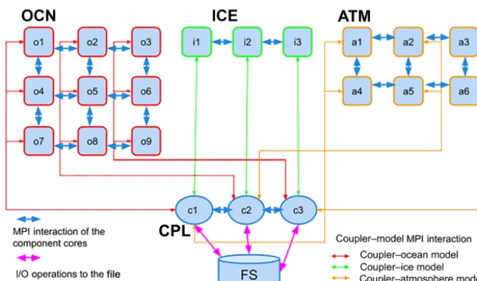
Figure 1.Architecture of the coupled model run under control of the CMF2.0. In this example there are three components (ocean, atmosphere, ice) connected by the 3-core coupler.
All events in the system are divided into a few classes (save diagnostics, save control point, read file data, send/receive mapping, etc.), defining different actions with data arrays. In the CMF2.0, we postulate that all events could be prede-fined before the start and occur with fixed periods. Thus, the coupler can take on the task of synchronizing models and avoiding deadlocks.
The sequence of events (time chain) is constructed in the main CMF program, which is the entry point of the cou-pled model. Also, at the registration stage, models provide the CMF system with pointers to the arrays that must be processed in the events. So, during the system operation, events are performed automatically and do not require ex-plicit calls from the user. As the information about the peri-ods of all events is known at the registration stage, the cou-pler can build a table of its actions. This allows one to ex-clude parallel synchronization of the coupler cores, which otherwise would be necessary when, for example, two com-ponents at the same time want to write data to the file sys-tem. When a certain time moment arrives, the coupler se-lects the next event from the chain and calls the appropri-ate handler function based on the type of this event, while the model components asynchronously send data. Moreover, it becomes possible to use persistent MPI operations (com-binations ofMPI_SEND_INITandMPI_STARTALL) for all events, thus saving time for repeated communications. The combination of predefined time chain, persistent commu-nications and pointer-based asynchronous sending provides high efficiency of parallel data gathering and distribution. 3.3 Coupler mapping
The interpolation algorithm uses SCRIP-formatted weight files built at the pre-run (off-line) stage by means of the
Cli-mate Data Operators (CDO) package (http://mpimet.mpg.de/ cdo, last access: 25 September 2018). At the beginning of the run stage, the weight files are read by the coupler in parallel. During the run, the data intended for mapping is sent by each component core to its master core asynchronously, without blocking.
The regridding process is performed in the coupler com-municator and is implemented as a sparse matrix – vector multiplication. It supports logically rectangular grids. We implemented the “source” and “destination” parallel map-ping algorithms (Craig et al., 2005), which correspond to the weights being distributed according to the destination or source grid decomposition, respectively. The former is usu-ally more efficient if the source grid has fewer points than the destination one, and the latter vice versa.
The SCRIP format is used to organize the mapping pro-cess, i.e., SCRIP-type links connect cells of destination and source grids with appropriate weights. Since every coupler core works only with a subdomain of the global model grid, it has only a part of the source grid data in memory. Other data should be gathered from neighboring cores during every interpolation event, which is functionally analogous to call-ing the “Rearranger” routines of Jacob et al. (2005). Both the component–component SCRIP links and intra-coupler rear-range routes are initialized at the beginning of the run and used at the run stage as persistent.
which could be the case when a source cell is used in a few destination cells. As a result, there is an overlap of compu-tations and communications, which, in conjunction with per-sistent MPI transactions, determines the high efficiency of the algorithm.
The performance rate of the CMF2.0 interpolation sys-tem was evaluated in several “ping-pong” tests, in which the coupler was ensuring component–component exchanges of the INMIO-SLAV ocean–atmosphere model with disabled solvers of physics equations (similarly to the ping-pong test of OASIS3 in Valcke, 2013).
In Test I, the ocean model sends three 2-D fields every 2 h to the atmosphere model and receives nine 2-D fields every 1 h. The ocean model has the 3600×1728 tripolar grid and the atmosphere model has the 1600×864 latitude– longitude grid (grids were taken from the current versions of ocean; Ibrayev et al., 2012; and atmosphere; Tolstykh et al., 2017; models). The mapping process consists of gath-ering data from the source component, regridding inside the coupler communicator and distributing the result to the des-tination component. The test was run for 10 model days, which corresponds to 120×3 ocean–atmosphere mappings and 240×9 atmosphere–ocean mappings. Sizes of commu-nicators for the ocean and atmosphere model components were fixed by 1152 and 288 cores, respectively. While not performing any computational work, they allow one to imi-tate real communication load of the overall system, reflecting packing, MPI sending and unpacking costs. Thus, the charts present a strong scalability of the coupler interpolation algo-rithm.
Results were obtained on four supercomputers: MVS-100k, MVS-10P, BlueGene/P and BlueGene/Q (characteris-tics are provided in the Appendix). On all supercomputers, the coupled system was compiled with a standard Intel For-tran compiler. Timing results of the 10-day Test I on MVS supercomputers are presented in Fig. 2. Two configurations, with 16 real and 32 virtual cores per node, are shown for the MVS-10P. The difference in the speed of their work is ex-pected and is a result of increased communication load for a larger number of cores per node. The graph shows good scalability with increasing size of the coupler communicator. The best result of 1 second is achieved at 288 coupler cores. It is clear that 20–40 coupler cores provide a satisfac-tory speed for such problems, because a cost of ∼10 s for 10 model days is a rather insignificant value for the high-resolution ocean–atmosphere coupled modeling. The figure also shows the ineffectiveness of the sequential algorithm: even on the fast MVS-10P processors the service activity takes about 200 s. Besides, the work of the sequential algo-rithm is only possible if all the node memory is allocated for the interpolation block, which is unlikely in practice (in our test we had to switch off physical model array allocation). Good coupler performance for one component–component connection is necessary for overall performance with a grow-ing number of components and their grid resolution.
Figure 2. Wall-clock time required for the 10-day ocean– atmosphere model run with disabled physics vs. number of coupler cores on MVS supercomputers (Test I for CMF2.0).
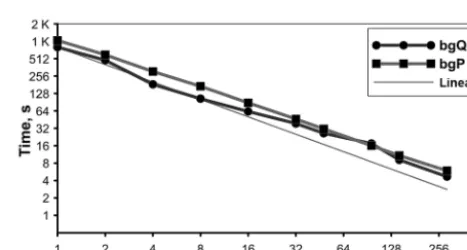
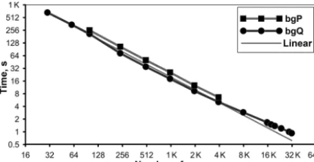
Figure 3. Wall-clock time required for the 10-day ocean– atmosphere model run with disabled physics vs. number of coupler cores on BlueGene supercomputers (Test I for CMF2.0).
Results of the same test for the BlueGene supercomputers are presented in Fig. 3. Timing of the algorithm is weaker than on the MVS-10P because of lower individual processor rate.
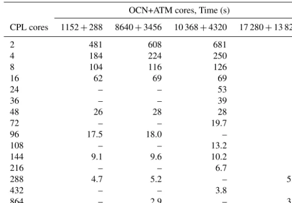
Test II was conducted for estimation of the increasing communication load associated with the growth of compo-nents’ communicator sizes. The timing still refers to the 10-day experiment with disabled physics. But the model grids were decomposed on a much higher number of subdomains, increasing the cost of the gather/distribute phase of the test (mapping process inside the coupler communicator remains the same). The results are shown in Fig. 4 (curves replaced by point symbols to improve the readability of the graph) and, for convenience, repeated in the Table 1. The number of cores used for the ocean and atmosphere models were equal to 8640 and 3456, 10 368 and 4320, and 17 280 and 13 824, respectively.
Table 1.The same data as in Fig. 4, with added BlueGene/Q data from Fig. 3.
OCN+ATM cores, Time (s)
CPL cores 1152+288 8640+3456 10 368+4320 17 280+13 824
2 481 608 681 –
4 184 224 250 –
8 104 116 126 –
16 62 69 69 –
24 – – 53 –
36 – – 39 –
48 26 28 28 –
72 – – 19.7 –
96 17.5 18.0 – –
108 – – 13.2 –
144 9.1 9.6 10.2 –
216 – – 6.7 –
288 4.7 5.2 – 5.0
432 – – 3.8 –
864 – 2.9 – 3.1
– denotes not tested or unsupported configurations
Figure 4. Wall-clock time required for the 10-day ocean– atmosphere model run with disabled physics vs. number of coupler cores on BlueGene/Q supercomputer, for different decomposition sizes of the ocean and atmosphere models (Test II for CMF2.0).
times for two coupler cores for model communicator sizes (8640, 3456) and (10 368, 4320) are correspondingly 26 % and 42 % higher than for Test I communicator sizes (1152, 288). For eight coupler cores this difference becomes 12 % and 21 %, correspondingly. Since every coupler core com-municates only with a subset of component cores, increas-ing of the coupler communicator size leads both to decom-posing of the interpolation computations and to decreasing of the component–coupler communication overhead, though slightly increasing intra-coupler rearrangement communica-tions. As a result, even a few tens of coupler cores are suit-able to provide good performance of high-resolution map-ping with huge sizes of model communicators.
3.4 Input/output scheme
Since the speed of I/O operations in supercomputers is often slow, writing large amounts of data (such as control points that include several 3-D arrays) can take an unacceptably long time. In the case of frequent data dumps or a slow file system, the time of calculations could be even comparable to the time of I/O, thus it is very important to optimize interac-tion with the file system. Its realizainterac-tion can be synchronous (blocking) or asynchronous (non-blocking) (e.g., see Balaji et al., 2017).
In the former case, I/O operations are performed by some subset of the processor cores of physical model components, thus inhibiting the physical equations solving.
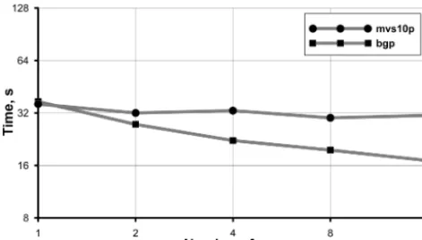
Figure 5.Wall-clock time of parallel writing of a model array of 4096×2048×50 size by different numbers of CMF2.0 coupler cores on MVS-10P and BlueGene/P supercomputers.
The asynchronous approach is generally more flexible, so it was chosen for the CMF. In the CMF2.0, all I/O actions are performed by the coupler. The realization is fully parallel, so one can work with any grid size by just increasing the number of coupler cores. Test results of the CMF2.0 I/O system for the case of writing a single-precision model array of 4096×
2048×50 size are shown in Fig. 5.
It can be seen that the writing speed of MVS-10P is ap-proximately constant. Moreover, the timing does not change when writing cores are allotted on one or several nodes. The reason is that MVS-10P has only one I/O node and all file operations are performed through it. On the other hand, the BlueGene/P system has several I/O nodes, so a reduction in the writing time is obtained when increasing the number of coupler cores. Nevertheless, the main advantage of the CMF I/O system is its asynchrony and memory scalability. The ac-celeration obtained with the BlueGene/P system is rather a nice particular result than a permanent CMF feature. It draws attention to the need of developing I/O infrastructure on su-percomputer systems. It is obvious that scalability graphs of a future exaflop machine with millions of cores become very artificial if one has to work with the file system through a single channel.
3.5 Additional features
Apart from the coupler, the framework also includes two helpful blocks. For the pre-run stage, the CMF2.0 has got the off-line block, which constructs SCRIP interpolation weights and prepares initial condition files. Like the run-stage CMF program, it is implemented in terms of abstract operations, which reduces all model configuration actions required from the user (e.g., grid definition) to realization of a few abstract interfaces in a user-derived class.
At the run stage, the user can call various utility mod-ules, like the HaloUpdater, which is needed in finite-difference models. It uses a 4-neighbor scheme of any length/dimension/type update on latitude–longitude and
tripolar grids, still handling diagonal cells. Impact of the HaloUpdater on performance of the INMIO WOM is de-scribed later.
Also, the CMF2.0 provides helpful tools for automatic building of various model combinations, makefile and skele-ton class generation, data preprocessing, and for other infras-tructure actions.
4 CMF3.0
4.1 PGAS abstraction
The CMF2.0 has shown itself as a suitable framework for high-resolution coupled modeling, allowing us to perform long-term experiments which would be impossible without it. But the CMF2.0 still has several points for improve-ment. First of all, although the pure MPI-based messaging is quite fast, it needs explicit work with sending and re-ceiving buffers. Additionally, development of nested regional models becomes quite difficult using only MPI routines. The CMF2.0 test results showed that we can easily sacrifice some performance and choose better (but perhaps less computa-tionally efficient) abstraction to simplify messaging routines. We have chosen the Global Arrays library (GA), which implements the Partitioned Global Address Space (PGAS) paradigm of parallel communication and provides an inter-face that allows one to distribute data while maintaining the type of global index space and programming syntax simi-lar to that available when programming on a single proces-sor (Nieplocha et al., 2006). The general idea is to give the user easy access to different parts of a distributed array. The PGAS abstraction assumes that there is a virtual huge array, which is accessible from any process involved in its creation. In fact, there is no global array, and its parts are stored lo-cally in the memory of processes. But the user does not know about it, since the library takes over all the details, due to which the simplicity is achieved. For example, the client on processXmay request an array element with indexes [i,j], as if it has direct access to it. Behind the scenes, GA learns which process holds this element (processY), executes MPI send–receive transfer and returns the result to the client.
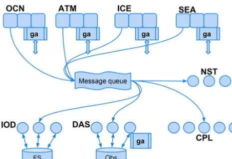
Figure 6. The architecture of the compact framework CMF3.0. There are four components in this example: ocean model (OCN), ice model (ICE), atmosphere model (ATM) and sea model (SEA). The components send requests to the common message queue, from where they are retrieved by the coupler (CPL), data assimilation (DAS), input and output data (IOD), and nesting (NST) services. The data itself is transferred through the mechanism of global ar-rays, which is also used for inter-processor communications in the components and services.
to/from the global array (this operation is local since the global arrays’ processor-wise allocation perfectly matches the model decomposition) and continues calculations. Ser-vice components get the array from the other side, but this time on their own decompositions. For example, the ocean component could store a global array on 5000 cores with some 2-D decomposition, while the I/O procedure outputting this array could utilize only four cores and a 1-D decompo-sition.
4.2 SOA architecture
As the complexity of coupled models is growing, we need an easy and convenient way of connecting model compo-nents together. The SOA, which was originally introduced for web applications, gives a good pattern for component in-teractions. In the CMF3.0, all model components send their requests to the common message queue. The service com-ponents only receive the messages they could process, then get data from appropriate global arrays and perform the re-quired actions. Such an architecture allows us to minimize dependencies between physical and service components, and makes development much easier. Moreover, since all services in the CMF3.0 are based on the same template (inherit the base class Service), it also allows the user to easily add new services to the system by filling only few abstract interfaces. Today, we have four completely independent services built into the CMF3.0: CPL (mapping), IOD (I/O service), NST (nesting service) and DAS (data assimilation service).
The CPL service represents the coupler from the CMF2.0 and serves all mapping requests. It receives data through the Communicator_GA class routines, performs interpola-tion and pushes data to the destinainterpola-tion global array (with-out a request from the receiving side). Although the central coupler architecture of CMF2.0 allows one to collect all ser-vice operations on one external component and to perform each of them in parallel, simultaneous requests can some-times lead to inefficient usage of processor time. For exam-ple, the CMF2.0 coupler can not perform parallel mapping and parallel I/O operations together. This is a disadvantage of all data transfer schemes that combine two or more ac-tions on one process.
In the CMF3.0, we decided to pick out a separate I/O ser-vice, only responsible for working with the file system. For example, when writing data to a file, on the component side it works as follows: the model component has to wait until the corresponding GA array is free, put the data into the GA array, mark the GA array as full and send request for the IOD service. On the IOD side, the request is read by the service, the service then takes the requested data from the GA array and marks the array as free; calls NetCDF routines (same as in the CMF2.0) for parallel writing to file. This approach, though not expected to perform faster than the CMF2.0 direct MPI messaging, provides a flexible and fully asynchronous data writing, limited mainly by the bandwidth of the file sys-tem.
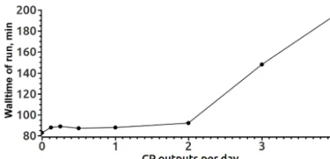
A performance test of the CMF3.0 I/O system in the IN-MIO World Ocean model of 0.1◦ resolution is shown in Fig. 7. In this test we compare the wall-clock times of 8-day ocean model runs (full physics equations solving) on 600 ocean and 10 IOD cores of the MVS-10P system with different frequencies of solution control point (CP) writing to file. The frequencies range from one CP per 6 model hours to one CP per 8 days, the case of no output is also exam-ined. One CP output (file of size 8 GB) takes about 5 wall-clock minutes, while one model day physics calculations take about 10 min, so one may expect that overlapping of compu-tation and output will be possible if CPs are written no more often than twice a model day. Indeed, we see that the graph shows linear growth of required run time if output frequency is greater than 2 CPs per day. This is a quite satisfactory value for long-term experiments such as in Earth climate studies (e.g., Marzocchi et al., 2015; where (1/12)◦ global ocean model outputs are stored as successive 5-day means).
It should be noted that one external I/O service solves only part of the problem, because in the case of writing large CP files and dumping frequent lightweight diagnostics the model still would be blocked by the former. Therefore, the service may be further split into two parts – fast and slow I/O-devices. Due to the abstract structure of the Service class this separation can be done via a few lines of code.
Figure 7.Wall-clock time of an 8-day run of INMIO World Ocean model with 0.1◦resolution vs. frequency of saving solution control points.
new DAS service, which implements the logic of parallel data assimilation (Kaurkin et al., 2016a, b).
4.3 The Communicator_GA class
The Communicator_GA is a CMF3.0 system class that rep-resents a kind of facade for the GA library. That is, it defines a high-level interface and hides some subtleties of the GA from the user. For example, the class allows one to create an array that will be distributed on one component, but still visible to another component. It can be a temperature array that is physically distributed over the ocean’s cores (and they can read and write data to it), but, in addition, the CPL ser-vice can also work with this array, although it does not store any part of it. Creation of such a global array in CMF3.0 will require just a few subroutine calls:
– request the CMF system for component identifiers and process lists of currently running ocean model and CPL service;
– register this joint group of processes, prescribing ocean as the holder and CPL as the subscriber;
– request the system for current ocean decomposition; – register the array, specifying the ocean as the holder and
passing its decomposition (so that GA distributes the mirror array in the same way as the model component does with the original one), and the coupler as the sub-scriber.
The GA put and get operations may now be called. For the holder side they will be local due to consistency of the de-composition. One of the benefits of this architecture is that now the model decomposition can be arbitrary. For example, it becomes easy not to reserve processor cores for subdo-mains of an ocean model that lay on land.
Every put/get operation must maintain explicit synchro-nization by setting the array status accordingly to “full” or “empty”. This is required since we are not allowed to “lose data”. That is, even if some component (e.g., ocean model)
is faster than another component (atmosphere model, or IOD in the case of too frequent data dumps), we must not lose an array. Accumulation of arrays in a queue also will not lead to success, since models usually work at constant speeds and, as a result, the queue will soon exhaust all available memory. So, if the “fast” model is ready to put/get data, but the GA array is still occupied/empty, the model is blocked.
4.4 Interpolation
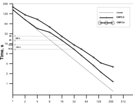
Since the logic of interpolation subroutines in the CMF3.0 remains the same as in the CMF2.0, we can greatly simplify it by use of GA abstractions. Now, all source data needed by the destination cell is collected directly by Communica-tor_GA routines. The optimizations regarding repeated cells are preserved. Disadvantage of using the GA is a decrease in performance, since it can not provide persistent operations, overlapping of computations and communication in one ser-vice, and obviously has its own overheads. We take the same parameters and input files as of the Test I to compare the CMF3.0 performance with that of the CMF2.0 (Fig. 8). Again, we measure the overall timing including costs of sending event request, sending data, interpolation process and pushing data into destination arrays. Therefore, this tim-ing reflects the overall system overhead against the timtim-ing of physical model components.
Tests were conducted on the MVS-10P supercomputer configuration with 16 cores per node. The graph shows that results are not as good as those for the CMF2.0 (Fig. 2 curve mvs10p_16 is repeated here), but the linear scalability trend is preserved. Moreover, the rate of 2–3 s per modeling day (on 20–50 CPL cores) is quite satisfactory for our practical purposes in high-resolution numerical experiments. The de-cline in performance is expected due to the overhead of using GA arrays (as an intermediate send/receive data representa-tion) and due to deprecated MPI_SEND_INIT procedures in the CMF3.0. This is a sacrifice for the compact code repre-sentation and for convenience of adding new features. 4.5 Additional features
Figure 8. Wall-clock time required for the 10-day ocean– atmosphere model run with disabled physics vs. number of cou-pler cores on the MVS-10P supercomputer (Test I for CMF2.0 and CMF3.0).
prescribed forcing referenced to the real calendar, e.g., the Drakkar forcing set; Dussin et al., 2016). Depending on cur-rent model time, these objects send requests or do nothing. Generators are realized by an abstract class, so for new spe-cific events generator subclasses could be easily added.
In case of unexpected behavior (like exceptions in model physics or changes in external data) the user can directly call the raise event routine, e.g., for emergency data dump or even to change the functioning of other model components by spe-cial messages.
The first to respond to an event is the model component itself – it looks at the event’s type and determines what to do (e.g., in the case of saving diagnostics: put the data into the GA array, mark it as full, send a request to the services and continue running). Then, the event is packed into an MPI message and sent as a request to all services (if the model has decided to send it). Services unpack the event, look at its name, and either process it, or ignore.
Other parallel utilities implemented in the CMF3.0 include – array operations, such as resizing, changing index order, converting to string and back, search for a particular el-ement;
– calculating global sums and area integrals over a de-composed model field, which is important in maintain-ing conservation in geophysical fluid models (e.g., to correct the precipitation, evaporation and runoff alge-braic sum in stand-alone ocean simulations like; Griffies et al., 2012);
– memory usage monitoring.
In the CMF3.0, we included all pre- and post-processing utility modules available in CMF2.0. It is not difficult to
mi-grate from the CMF2.0 to the CMF3.0. Only one adapter file, about 200 lines of code, should be rewritten. It contains sev-eral procedures (ini_main, make_step, finalize, etc), besides defining events and arrays (intended for I/O, remapping, etc.) registered in it.
5 CMF examples of usage
There are several examples of using CMF for various geo-physical numerical models:
1. Eddy-resolving ocean dynamics modeling using the INMIO WOM with 0.1◦ resolution, governed by the CMF2.0 (Ibrayev et al., 2012; Ushakov and Ibrayev, 2018).
2. Data assimilation of satellite observations and ARGO float measurements using the DAS service in forecast and reanalysis experiments with the INMIO WOM gov-erned by the CMF3.0 (Kaurkin et al., 2016a).
3. There is a set of works with coupled atmosphere– ocean models for climate change research and numer-ical weather prediction. The SLAV global atmosphere model (Tolstykh et al., 2017) and the INMIO WOM (Ibrayev et al., 2012) were coupled using the CMF2.0 and CMF3.0 (Fadeev et al., 2016). The results of numer-ical experiments with the coupled model demonstrate agreement with observational data and show a possibil-ity to use this model for probabilistic weather forecasts at timescales from weeks to year.
4. The nesting technology implemented in the CMF3.0 NST service has been tested for the local INMIO-based model of the Barents Sea with a resolution of 0.1◦and the INMIO WOM with a resolution of 0.5◦with differ-ent geophysical parameterizations (Koromyslov et al., 2017).
5. First results of the seasonal variability simulation for the Arctic and North Atlantic ocean waters and ice by the coupled INMIO WOM and a sea-ice CICE5.1 (Turner and Hunke, 2015) models were obtained under the CMF2.0 in Ushakov et al. (2016). The numerical ex-periments were performed in conditions of the CORE-II protocol.
5.1 INMIO World Ocean model
Figure 9. Wall-clock time of the 0.1◦ resolution INMIO WOM (governed by the CMF2.0) 10 model steps vs. model communi-cator size on the BlueGene/P supercomputer (Moscow State Uni-versity) and BlueGene/Q supercomputer (IBM Research Center Thomas J. Watson).
only local halo updates. Therefore, limitations in scalability can only be associated with halo update routines and external blocks (e.g., in the I/O system).
The latest version of INMIO WOM is distributed in an in-tegrated package together with the CMF2.0 and 3.0, all nec-essary libraries and a standardized folder structure facilitat-ing the addfacilitat-ing of new model components (includfacilitat-ing adapter files for the Los Alamos Community Ice CodE (CICE) sea-ice model). At present, the INMIO code consists of the hy-drodynamical solver, atmospheric boundary layer bulk for-mulae, the built-in thermodynamic ice model of Schrum and Backhaus (1999) (turned off in the case of coupling with the CICE model), and online data processing routines (e.g., av-eraging). The intra-model communications (halo exchanges on tripolar and latitude–longitude grids) and work with the file system are delegated to the CMF utilities module. For prescribed experiments with the CORE (Griffies et al., 2012) forcing, two data models (reading CORE data files) are also registered as separate atmosphere and land components, and the CMF coupler provides interpolation of their fields onto the ocean grid.
Scalability of the INMIO WOM of 0.1◦resolution driven by the CMF2.0 is shown in Fig. 9. The maximum number of BlueGene/Q cores utilized is 32 400 (32 000 for the ocean component and 400 for the coupler). The parallel efficiency of this configuration in relation to the configuration of 8100 cores (8000 for the ocean and 100 for the coupler) is 78 %. Obviously, at high core counts the parallel efficiency curve experiences some “flattening”. But assuming that the time step of the model is 5 min., the result of the experiment leads to, for example, quite satisfactory a rate of 5 simulated years per wall-clock day (SYPD) achieved on 20 000 cores of the BlueGene/Q supercomputer.
5.2 Coupled global atmosphere–ocean model
The second application of the framework was the numerical experiment with the global coupled INMIO ocean (Ibrayev et al., 2012) and SLAV atmosphere (Tolstykh et al., 2017) models. The SLAV model with horizontal resolution 0.9◦×
0.72◦and 28 vertical levels, and the INMIO WOM with res-olution 0.25◦and 49 vertical levels were coupled into a sin-gle program using the CMF2.0 system. The short- and long-wave radiation in the SLAV model were computed with the time step of 1 h. The spatiotemporal resolution was restricted by available computer resources but not by the CMF itself.
Prognostic coupled model calculations were carried out with a time step of 6 min for the oceanic component and 3.6 min for the atmospheric one. The initial state of the ocean was obtained by a spin-up of the stand-alone ocean model driven by the ERA-Interim atmospheric forcing. The atmo-sphere started from the objective analysis of the Hydromet-center of Russia. Every 72 min, nine 2-D arrays were trans-ferred from the atmosphere to the ocean (components of wind stress, short- and long-wave radiation, fluxes of sensible and latent heat, precipitation, evaporation and air tempera-ture at 2 m). Conversely, every 144 min three 2-D arrays were transferred from the ocean to the atmosphere (upper grid-box temperature, temperature and concentration of sea ice). The sea ice was simulated by the INMIO built-in ice thermody-namics model, while the land processes were incorporated into the SLAV atmosphere model. The coupled model works stably and, along with intra-annual distribution characteris-tics of monthly data fields, reproduces enough thin elements of atmospheric and oceanic circulation.
The model throughput on the MVS-10P supercomputer was equal to 0.75 SYPD for the configuration ocean (1152 cores) – atmosphere (288 cores) – coupler (16 cores). At that moment, the maximal communicator size available for the atmosphere model was limited due to the one-dimensional latitudinal grid decomposition.
5.3 Data assimilation using DAS
Figure 10. Scalability of the EnOI method in the context of the CMF3.0 DAS service at the assimilation of 104 points on the Lomonosov supercomputer (Moscow State University).
Due to the effective implementation of the EnOI method as the DAS parallel software service, the data assimilation prob-lem scales almost linearly (Fig. 10). So, assimilation of 104 observational points of satellite data on 16 processor cores takes about 20 s instead of 5 min on a single core, which would be comparable to the time spent on daily ocean model forecast for 200 cores.
6 Summary and conclusions
We present an original modeling framework CMF developed as our first step to high-resolution modeling. The key part of it, the coupler, in the initial version CMF2.0 has a suffi-ciently small code size for such programs (about 5000 lines of code including unit tests) and is able to manage the main parallel problems of the coupled modeling – synchroniza-tion, regridding and I/O. The coupled model follows the sin-gle executable design with the main program independent of components’ code, and the coupler dealing with all service operations. The new version, CMF3.0, utilizes the SOA de-sign, which allows one to divide the coupler responsibilities into small separate services, easily plug/unplug them and add new ones to the system, thus providing a further generaliza-tion to the coupling interface. The PGAS messaging greatly simplifies implementation of all model low-level interprocess communications.
Tests for CMF2.0 parallel mapping efficiency were car-ried out on four modern supercomputer architectures. They show a nearly linear scalability of the overall communication system and the regridding procedure. Satisfactory speed re-sults could be achieved already on 20–40 coupler cores even dealing with grids of high resolution (0.1◦for the ocean and 0.225◦for the atmosphere). I/O tests proved the ability of the coupler asynchronous I/O scheme to handle huge amounts of data. As expected, the new CMF 3.0 version has lower absolute performance, but still preserves the linear trend of scalability and suitable timing (2–3 s per modeling day on 20–50 coupler cores) for high-resolution modeling. The par-allel data output speed of CMF3.0 is about a half of that for CMF2.0, but still it is quite satisfactory for contempo-rary high-resolution climate experiments due to overlapping of computation and writing to the file system. Within the framework of the CMF3.0 architecture it was possible to ef-fectively implement nesting and data assimilation technolo-gies. This functionality is not yet common for other coupling platforms.
Originally designed for the INMIO World Ocean model support, the CMF has developed into a flexible and extensi-ble instrument providing means for high-resolution resource-demanding simulations in regional to global, stand-alone or coupled, and forecast and climate problems.
Appendix A: Supercomputer configurations used The MVS-100k and MVS-10P systems are installed at the Joint Supercomputer Center of the Russian Academy of Sciences (www.jscc.ru, last access: 25 September 2018). The MVS-100k consists of 1460 modules (11 680 processor cores). The basic computing module is an HP Proliant server, containing two quad-core Intel Xeon processors running at 3 GHz on 8 GB RAM. Computational modules are intercon-nected with Infiniband DDR. The MVS-10P system includes 207 nodes. Each node incorporates two Intel Xeon E5-2690 processors (16 cores on 2.90 GHz), 64 GB of RAM, and two Intel Xeon Phi 7110H coprocessors. Computing nodes are combined into an FDR Infiniband network.
Supercomputer BlueGene/P is located at the Faculty of Computational Mathematics and Cybernetics, Moscow State University, and consists of 2048 computing nodes. Each node has four PowerPC 450 cores (850 MHz) and 2 GB of RAM. Nodes are networked with the 3-D torus topology (5.1 GB s−1, DMA).
Supercomputer BlueGene/Q is located at the IBM Thomas J. Watson Research Center and consists of several racks. Every two racks have 2048 computational nodes, each with 16 cores. The core is a PowerPC A2 (16 GB RAM, 1.6 GHz). Nodes are networked with the 5-D torus topology (40 GB s−1, DMA).
Author contributions. VK was responsible for most aspects of the CMF2.0 and CMF3.0 development, including design, code writ-ing, and testing. RI and KU designed and developed the INMIO model and physical coupling algorithms. MK was the CMF3.0 co-developer and the author of the Data Assimilation Service. VK wrote the first draft of the article, and all co-authors contributed to software validation, performance tests, and the final version of the article.
Competing interests. The authors declare that they have no conflict of interest.
Acknowledgements. The research of Sections 1–3, 5.1 and 5.2 was supported by the Russian Science Foundation (project no. 14-37-00053) and performed at the Hydrometeorological Research Center of the Russian Federation. The research of Sections 4 and 5.3 was supported by the Russian Science Foundation (project no. 17-77-30001) and performed at the Federal State Budget Scientific Institution “Marine Hydrophysical Institute of RAS”.
Edited by: Steve Easterbrook
Reviewed by: Sophie Valcke and one anonymous referee
References
Balaji, V.: The Flexible Modeling System, Springer Berlin Heidel-berg, Berlin, HeidelHeidel-berg, 33–41, https://doi.org/10.1007/978-3-642-23360-9_5, 2012.
Balaji, V., Maisonnave, E., Zadeh, N., Lawrence, B. N., Biercamp, J., Fladrich, U., Aloisio, G., Benson, R., Caubel, A., Durachta, J., Foujols, M.-A., Lister, G., Mocavero, S., Underwood, S., and Wright, G.: CPMIP: measurements of real computational perfor-mance of Earth system models in CMIP6, Geosci. Model Dev., 10, 19–34, https://doi.org/10.5194/gmd-10-19-2017, 2017. CESM: CESM1.2 User guide, NCAR, available at: http://www.
cesm.ucar.edu/models/cesm1.2/cesm/doc/usersguide/ug.pdf (last access: 25 September 2018), 2013.
Craig, A., Valcke, S., and Coquart, L.: Development and performance of a new version of the OASIS coupler, OASIS3-MCT_3.0, Geosci. Model Dev., 10, 3297–3308, https://doi.org/10.5194/gmd-10-3297-2017, 2017.
Craig, A. P., Jacob, R., Kauffman, B., Bettge, T., Larson, J., Ong, E., Ding, C., and He, Y.: CPL6: The New Extensible, High Performance Parallel Coupler for the Community Cli-mate System Model, Int. J. High Perform. C., 19, 309–327, https://doi.org/10.1177/1094342005056117, 2005.
Craig, A. P., Vertenstein, M., and Jacob, R.: A new flex-ible coupler for earth system modeling developed for CCSM4 and CESM1, Int. J. High Perform. C., 26, 31–42, https://doi.org/10.1177/1094342011428141, 2012.
Dennis, J. M., Edwards, J., Loy, R., Jacob, R., Mirin, A. A., Craig, A. P., and Vertenstein, M.: An application-level parallel I/O li-brary for Earth system models, Int. J. High Perform. C., 26, 43– 53, https://doi.org/10.1177/1094342011428143, 2012a. Dennis, J. M., Vertenstein, M., Worley, P. H., Mirin, A. A.,
Craig, A. P., Jacob, R., and Mickelson, S.: Computational
per-formance of ultra-high-resolution capability in the Commu-nity Earth System Model, Int. J. High Perform. C., 26, 5–16, https://doi.org/10.1177/1094342012436965, 2012b.
Dussin, R., Barnier, B., Brodeau, L., and Molines, J.: The making of the Drakkar forcing set DFS5, Tech. rep., DRAKKAR/MyOcean Report 01-04-16, LGGE, Grenoble, France, 2016.
Fadeev, R. Y., Ushakov, K. V., Tolstykh, M. A., Ibrayev, R. A., and Kalmykov, V. V.: Coupled atmosphere–ocean model SLAV– INMIO: implementation and first results, Russ. J. Numer. Anal. M., 31, 329–337, https://doi.org/10.1515/rnam-2016-0031, 2016.
Gamma, E., Helm, R., Johnson, R., and Vlissides, J.: Design Pat-terns: Elements of Reusable Object-oriented Software, Addison-Wesley Longman Publishing Co., Inc., Boston, MA, USA, 1995. Griffies, S. M., Winton, M., Samuels, B., Danabasoglu, G., Yea-ger, S., Marsland, S., Drange., H., and Bentsen, M.: Datasets and protocol for the CLIVAR WGOMD Coordinated Ocean-sea ice Reference Experiments (COREs), WCRP Report No. 21/2012, Tech. rep., 2012.
Ibrayev, R. A.: Model of enclosed and semi-enclosed sea hydrodynamics, Russ. J. Numer. Anal. M., 16, 291–304, https://doi.org/10.1515/rnam-2001-0404, 2001.
Ibrayev, R. A., Khabeev, R. N., and Ushakov, K. V.: Eddy-resolving 1/10◦model of the World Ocean, Izv. Atmos. Ocean Phy., 48, 37–46, https://doi.org/10.1134/S0001433812010045, 2012. Ibrayev, R. A., Ushakov, K. V., Kalmykov, V. V., Kaurkin, M. N.,
and Dyakonov, G. S.: Ocean Supercomputer Modeling Labora-tory, available at: http://model.ocean.ru, last access: 25 Septem-ber 2018.
Jacob, R., Larson, J., and Ong, E.:M×NCommunication and Par-allel Interpolation in Community Climate System Model Version 3 Using the Model Coupling Toolkit, Int. J. High Perform. C., 19, 293–307, https://doi.org/10.1177/1094342005056116, 2005. Jones, P. W.: First- and Second-Order Conservative
Remap-ping Schemes for Grids in Spherical Coordinates, Mon. Weather Rev., 127, 2204–2210, https://doi.org/10.1175/1520-0493(1999)127<2204:FASOCR>2.0.CO;2, 1999.
Kalmykov, V. V. and Ibrayev, R. A.: A framework for the ocean-ice-atmosphere-land coupled modeling on massively-parallel archi-tectures, Vychisl. Metody Programm., 14, 88–95, available at: http://mi.mathnet.ru/vmp156 (last access: 25 September 2018), 2013 (in Russian).
Kaurkin, M., Ibrayev, R., and Koromyslov, A.: EnOI-Based Data Assimilation Technology for Satellite Observations and ARGO Float Measurements in a High Resolution Global Ocean Model Using the CMF Platform, Communications in Computer and In-formation Science, Springer International Publishing, 687, 57– 66 https://doi.org/10.1007/978-3-319-55669-7_5, 2016a. Kaurkin, M. N., Ibrayev, R. A., and Belyaev, K. P.: ARGO data
as-similation into the ocean dynamics model with high spatial res-olution using Ensemble Optimal Interpolation (EnOI), Oceanol-ogy, 56, 774–781, https://doi.org/10.1134/S0001437016060059, 2016b.
Larson, J., Jacob, R., and Ong, E.: The Model Coupling Toolkit: A New Fortran90 Toolkit for Building Multiphysics Paral-lel Coupled Models, Int. J. High Perform. C., 19, 277–292, https://doi.org/10.1177/1094342005056115, 2005.
Marzocchi, A., Hirschi, J. J.-M., Holliday, N. P., Cunning-ham, S. A., Blaker, A. T., and Coward, A. C.: The North Atlantic subpolar circulation in an eddy-resolving global ocean model, J. Marine Syst., 142, 126–143, https://doi.org/10.1016/j.jmarsys.2014.10.007,2015.
Nieplocha, J., Palmer, B., Tipparaju, V., Krishnan, M., Trease, H., and Aprà, E.: Advances, Applications and Perfor-mance of the Global Arrays Shared Memory Program-ming Toolkit, Int. J. High Perform. C., 20, 203–231, https://doi.org/10.1177/1094342006064503, 2006.
Redler, R., Valcke, S., and Ritzdorf, H.: OASIS4 – a coupling soft-ware for next generation earth system modelling, Geosci. Model Dev., 3, 87–104, https://doi.org/10.5194/gmd-3-87-2010, 2010. Schrum, C. and Backhaus, J.: Sensitivity of atmosphere–ocean heat
exchange and heat content in the North Sea and the Baltic Sea, Tellus A, 51, 526–549, https://doi.org/10.1034/j.1600-0870.1992.00006.x, 1999.
Shukla, J.: World Modelling Summit for Climate Prediction. WCRP-131, WMO/TD-No.1468, UK, European Centre for Medium-Range Weather Forecasts, 2008.
Theurich, G., DeLuca, C., Campbell, T., Liu, F., Saint, K., Verten-stein, M., Chen, J., Oehmke, R., Doyle, J., Whitcomb, T., Wall-craft, A., Iredell, M., Black, T., Silva, A. M. D., Clune, T., Fer-raro, R., Li, P., Kelley, M., Aleinov, I., Balaji, V., Zadeh, N., Ja-cob, R., Kirtman, B., Giraldo, F., McCarren, D., Sandgathe, S., Peckham, S., and IV, R. D.: The Earth System Prediction Suite: Toward a Coordinated U.S. Modeling Capability, B. Am. Mete-orol. Soc., 97, 1229–1247, https://doi.org/10.1175/BAMS-D-14-00164.1, 2016.
Tolstykh, M., Shashkin, V., Fadeev, R., and Goyman, G.: Vorticity-divergence semi-Lagrangian global atmospheric model SL-AV20: dynamical core, Geosci. Model Dev., 10, 1961–1983, https://doi.org/10.5194/gmd-10-1961-2017, 2017.
Turner, A. K. and Hunke, E. C.: Impacts of a mushy-layer ther-modynamic approach in global sea-ice simulations using the CICE sea-ice model, J. Geophys. Res.-Oceans, 120, 1253–1275, https://doi.org/10.1002/2014JC010358, 2015.
Ushakov, K. V. and Ibrayev, R. A.: Assessment of mean world ocean meridional heat transport characteristics by a high-resolution model, Russ. J. Earth Sci., 18, ES1004, https://doi.org/10.2205/2018ES000616, 2018.
Ushakov, K. V., Grankina, T. B., Ibrayev, R. A., and Gromov, I. V.: Simulation of Arctic and North Atlantic ocean water and ice seasonal characteristics by the INMIO-CICE coupled model, IOP Conference Series: Earth and Environmental Science, 48, 012013, https://doi.org/10.1088/1755-1315/48/1/012013, 2016. Valcke, S.: The OASIS3 coupler: a European climate
mod-elling community software, Geosci. Model Dev., 6, 373–388, https://doi.org/10.5194/gmd-6-373-2013, 2013.
Valcke, S., Balaji, V., Craig, A., DeLuca, C., Dunlap, R., Ford, R. W., Jacob, R., Larson, J., O’Kuinghttons, R., Ri-ley, G. D., and Vertenstein, M.: Coupling technologies for Earth System Modelling, Geosci. Model Dev., 5, 1589–1596, https://doi.org/10.5194/gmd-5-1589-2012, 2012.