https://doi.org/10.5194/gmd-12-4901-2019 © Author(s) 2019. This work is distributed under the Creative Commons Attribution 4.0 License.
WAVETRISK-1.0: an adaptive wavelet hydrostatic dynamical core
Nicholas K.-R. Kevlahan1and Thomas Dubos2
1Department of Mathematics and Statistics, McMaster University, Hamilton, Canada 2Laboratoire de Météorologie Dynamique, École Polytechnique, Palaiseau, France Correspondence:Nicholas K.-R. Kevlahan ([email protected])
Received: 12 April 2019 – Discussion started: 16 May 2019
Revised: 16 October 2019 – Accepted: 25 October 2019 – Published: 27 November 2019
Abstract. This paper presents the new adaptive dynamical corewavetrisk. The fundamental features of the wavelet-based adaptivity were developed for the shallow water equa-tion on the β plane and extended to the icosahedral grid on the sphere in previous work by the authors. The three-dimensional dynamical core solves the compressible hydro-static multilayer rotating shallow water equations on a mul-tiscale dynamically adapted grid. The equations are dis-cretized using a Lagrangian vertical coordinate version of thedynamicomodel. The horizontal computational grid is adapted at each time step to ensure a user-specified relative error in either the tendencies or the solution. The Lagrangian vertical grid is remapped using an arbitrary Lagrangian– Eulerian (ALE) algorithm onto the initial hybridσ -pressure-based coordinates as necessary. The resulting grid is adapted horizontally but uniform over all vertical layers. Thus, the three-dimensional grid is a set of columns of varying sizes. The code is parallelized by domain decomposition using mpi, and the variables are stored in a hybrid data structure of dyadic quad trees and patches. A low-storage explicit fourth-order Runge–Kutta scheme is used for time integration. Val-idation results are presented for three standard dynamical core test cases: mountain-induced Rossby wave train, baro-clinic instability of a jet stream and the Held and Suarez sim-plified general circulation model. The results confirm good strong parallel scaling and demonstrate that wavetrisk can achieve grid compression ratios of several hundred times compared with an equivalent static grid model.
1 Introduction
main added value of AMR is its ability to accurately cap-ture events that are highly localized in space and time at a relatively low computational cost. Jablonowski et al. (2009) evaluated a block-structured AMR method for scalar two-dimensional transport on the sphere. Refinement and coars-ening levels are constrained so that there is a uniform 2 : 1 mesh ratio at all fine-grid/coarse-grid interfaces. In a series of test cases, they find that the additional resolution helps pre-serve the shape and amplitude of the transported tracer while saving computing resources in comparison to uniform-grid model runs. Kopera and Giraldo (2014) evaluated the perfor-mance of AMR in a discontinuous Galerkin-based implicit– explicit (IMEX) model on a planar two-dimensional grid. They found that AMR could provide up to a 15×speedup with minimal overhead. Ferguson et al. (2016) analyzed the performance of an AMR model for the shallow water equa-tions on the cubed sphere. Their model is built using the gen-eral purpose Chombo-AMR toolbox of finite difference and finite volume methods for the solution of partial differential equations on block-structured adaptively refined rectangular grids. They test the model for one or two levels of refinement with refinement ratios of ×2, ×4 and ×8 between each level. In comparison,wavetriskcurrently uses a fixed re-finement ratio of×2, but has been tested for up to six levels of refinement. Ferguson et al. (2016) conclude that AMR can be effective provided that a sufficiently fine coarsest grid is selected.
Beyond its ability to accurately capture events that are quite localized in space and time at a low cost, several ad-ditional properties are required for AMR to be an attrac-tive option for atmospheric applications. Firstly, AMR must demonstrate its ability to accurately simulate complex three-dimensional flows, where a large number of important fea-tures such as cyclones and waves continuously appear, move and disappear. Wavetriskhas already demonstrated this ability for (two-dimensional) shallow water flows. Further-more, especially for applications to climate modelling, the robustness of the method over long timescales and its abil-ity to capture accurate statistics should be shown. Finally, an efficient parallel implementation must be developed in order to compete with state-of-the art operational models. Skamarock and Klemp (1993) presented pioneering initial results from area-limited two- and three-dimensional AMR codes. Popinet et al. (2012) reported results for a three-dimensional AMR code on the cubed sphere at a conference, and Ferguson (2018)’s thesis also describes the develop-ment of a global three-dimensional AMR code (based on the CHOMBO library). However, although these groups made significant progress in developing global three-dimensional AMR, to the best of our knowledge, no AMR for complex three-dimensional atmospheric flows has been fully docu-mented and analyzed in a peer-reviewed publication.
A key element to the robustness and accuracy of any AMR method is its refinement criterion, which decides when and where to coarsen or refine the computational grid.
Fergu-son et al. (2016) evaluate several ad hoc criteria and iden-tify appropriate ones for their numerical experiments. How-ever, they do not find any “clear strategy for establishing the best general refinement criteria”. In contrast,wavetrisk uses objective and clearly defined refinement criteria which control the multiscale relative error of the solution or of its tendencies as measured directly by the wavelet coefficients. Although this strategy is objective and clearly defined, since it is based solely on the normalized local approximation er-ror of the solution or tendencies, it is not sufficient to control more qualitative measures of error, such as the location of a vortex. In particular, this approach would need to be aug-mented when subgrid parameterizations are included, such as for cloud formation or turbulence. Other refinement indi-cators would be appropriate when consideringprefinement (Naddei et al., 2019).
In the following section, we review briefly the basic prop-erties and computational features of the wavelet-based dy-namical adaptivity laid out in Dubos and Kevlahan (2013) and Aechtner et al. (2015). Section 3 summarizes the dis-crete equations solved by the model and presents the arbi-trary Lagrangian–Eulerian (ALE) vertical coordinate. Sec-tion 4 applies the principle of wavelet-based adaptivity to the three-dimensional model. In Sect. 5, implementation details are given and the adaptive solver is evaluated using three test cases of increasing complexity. Section 6 concludes the pa-per.
2 The adaptive wavelet method 2.1 Wavelet adaptivity on the plane
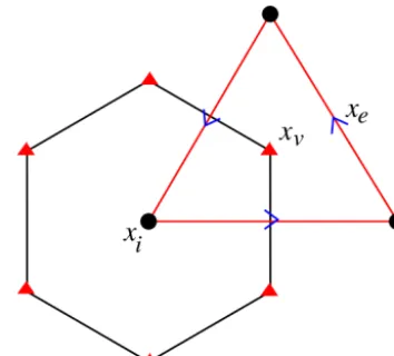
Figure 1.The regular C grid on the plane. Vorticity is located on the primal grid of triangles at points xv and mass located on the dual grid of hexagons at nodesxi. The velocities/fluxes are located on edges xe. A multiscale hierarchy of nested refined C grids is generated by bisecting the triangle edges.
Rµj◦divj+1=divj◦RjF conserves mass, (1) curlj◦Ruj=Rjζ◦curlj+1 conserves circulation, (2)
gradj◦RjB=Rju◦gradj+1 no spurious vorticity, (3)
whereRµ is mass density (or height) restriction,RF is the
flux restriction,Ru is the velocity restriction, Rζ is the
cir-culation (vorticity) restriction, andRBis the Bernoulli func-tion restricfunc-tion. The third commutafunc-tion relafunc-tion ensures that a flow with uniform potential vorticity remains uniform un-der the advection by an arbitrary velocity field (i.e. vorticity is advected like a tracer).
The C grid is a staggered grid where vorticity is located on triangles (the primal grid), and mass is located on the hexagons formed from the bisectors of the triangle edges (the dual grid). Velocity is located on the edges of triangles, which are also the perpendicular bisectors of the hexagonal edges. (Note that we have chosen the opposite notation to Ringler et al. (2010) and Dubos et al. (2015) since in the multiscale case the triangle grid is generated first by repeated bisection from the icosahedron and the hexagon grid is generated as the dual grid of the triangles.) The regular C grid is shown in Fig. 1. Starting with a coarsest grid, a multiscale hierarchy of primal grids is constructed by bisection of the triangle edges. The dual grid of hexagons is constructed from the perpendic-ular edge bisectors of the primal grid. On the plane, both the hexagons and triangles are nested and regular. We will see below that this is not the case for the sphere.
This hierarchy of computational grids leads to a so-called wavelet multiresolution analysis (MRA), i.e. the nested se-quence of approximation subspaces used to construct the second-generation biorthogonal wavelets (Sweldens, 1998) that are the basis of the grid adaptivity algorithm. The MRA
provides a sequence of smooth approximations of a function f (x)on each grid levelj and an associated sequence of “de-tails” which give the differences between the approximation at a fine levelj+1 and a coarse levelj. The details are ef-fectively the interpolation errors between scalesj+1 andj. The smooth approximation at scalej has a basis of scaling functions{φkj(x)}, while the details between scalesj+1 and jhave a basis of wavelets{ψkj(x)}.
If the wavelet coefficient at a particular position k and scalej is sufficiently small, i.e.|ψkj(x)|< ε, then the value of f (x)is well approximated by the function f≥(x) inter-polated from neighbouring scaling function values at the same scale. If the wavelet coefficient is large, the value of the wavelet coefficient (i.e. the details) must be retained and added to the interpolated value to obtain an sufficiently accu-rate approximation. Neglecting the small wavelet coefficients (and associated grid points) generates a multiscale hierarchy of adapted grids. The commutation relations (Eqs. 1–3) en-sure that the mimetic properties of the discretization are also satisfied on the adapted grid.
One can prove that this nonlinear wavelet filtering pro-vides error control:
||f (x)−f≥(x)||∞=O(ε), (4)
N=Oε−1/2N, (5)
||f (x)−f≥(x)||∞=O
N−2N, (6)
whereN is the number of grid points retained on the adapted grid andN is the order of interpolation. Thus, we can also estimate how many grid points (i.e. computational elements) are required to obtain an approximation with a desired error ε. Settingεtherefore determines the numerical error of the approximation (the tolerance) and also determines the num-ber of grid points in the adapted grid. In principle, it is not necessary to set a maximum resolution scaleJ since it is determined automatically byε. Note that an approximation f≥j(x)at each scalej is provided by the set of scaling func-tions{φjk}≥and their coefficients.
In previous work, we have shown that the CPU timeτnper
and Sreenivasan (2005) argue that temporal and spatial inter-mittency mean that turbulent flows require far higher resolu-tion than that found using the usual Kolmogorov-scale-based estimate,1x∼Re−3/4.
The above adaptive algorithm controls the error of the solution at each time step, but it does not allow for dy-namics. The solution can change over one time step from tn to tn+1t by translating at the same scale, coarsening (gradient weakens) or refining (gradient strengthens). If the Courant–Friedrichs–Lewy (CFL) criterion is 1, i.e. 1t < 1xmin/||u||∞, the solution can translate by a maximum of one grid point at the same scale over one time step. If the nonlinearities in the governing equations are quadratic, the active scale can increase by a maximum of a factor of 2 from j toj+1 over one time step. To allow for these changes, an “adjacent zone” is added to the set of active wavelet co-efficients{ψkj}≥that includes its nearest neighbours in both position and scale (Liandrat and Tchamitchian, 1990). The adaptive grid must also satisfy the perfect reconstruction cri-terion: there must be sufficient scaling functions (grid points) to construct the wavelets. There must also be sufficient grid points present at each scalejto construct the required TRiSK differential operators (by interpolation, if their associated wavelets are inactive). Once the new adapted grid has been constructed, the prognostic variables are interpolated onto the new grid by performing an inverse wavelet transform. After the solution is advanced, the wavelets on the union of the adapted grid and adjacent zone are again filtered using the thresholdεto obtain a new set of active wavelets at time tn+1t.
Because we use a staggered grid, the adaptive wavelet al-gorithm described above differs fundamentally from previ-ous adaptive wavelet collocation methods (e.g. Mehra and Kevlahan, 2008; Kevlahan and Vasilyev, 2005; Roussel and Schneider, 2010; Schneider and Vasilyev, 2010). Since mass and velocity are located at different points, we must construct two distinct wavelet transforms: a scalar-valued wavelet transform for mass density µ and a vector-valued wavelet transform for velocityu. To control the errors in the tenden-cies, the corresponding thresholdsεµandεu must be
prop-erly scaled. The details of these scalings in the inertia–gravity wave and geostrophic regimes are given in Dubos and Kevla-han (2013).
Finally, note that ideally the time step should also adapt to the local grid scale. In other words, the solution at each scale should be advanced on the time step1tj appropriate for that scale. Although this scale-dependent time stepping is optimal, in practice it does not provide much advantage unless only a small portion of the total active grid points is at the finest scale, which is not usually the case. Domingues et al. (2008) developed a second-order Runge–Kutta scale-dependent time stepping and McCorquodale et al. (2015) extended scale-dependent time stepping to arbitrary order. For simplicity, we have decided not to implement
scale-dependent time stepping inwavetrisk, although it could be added in the future.
The ability of the adaptive wavelet method to control the errors of the tendencies was verified in Dubos and Kevla-han (2013), and the computational performance and paral-lel efficiency of the method on the sphere were confirmed in Aechtner et al. (2015). Since the three-dimensional hy-drostatic code uses the multilayer shallow equations and horizontal adaptivity only, these properties are inherited by wavetrisk.
The prototypematlabserial implementation of the adap-tive algorithm in the plane is relaadap-tively straightforward be-cause the computational grid is uniform and we did not par-allelize the algorithm. In the following section, we review the extension of the algorithm to the sphere.
2.2 Wavelet adaptivity on the sphere
We have reviewed the essential elements of the adaptive wavelet method in the previous section; however, to be prac-tically useful for a dynamical core, the method must be ex-tended to the sphere and parallelized. The extension to the sphere presents numerous technical challenges. First, the grid is non-uniform, each computational element is geometrically unique, and the icosahedral grid on the sphere has 12 pen-tagonal dual grid cells (a sphere cannot be tiled uniformly). Secondly, the repeated bisection of the primal triangular grid used to generate the multiscale grid structure produces a grid that is increasingly distorted near the edges of the original icosahedron. Finally, the dual hexagonal grid is no longer nested between successive scales because the triangles used to generate it are not equilateral. This makes it complicated to construct the flux restriction from fine to coarse scales be-cause we must keep track of small overlapping regions. In the following, we focus on the most important modifications necessary to deal with the non-uniform geometry and to par-allelize the code in the following.
The wavelet transform on the non-adaptive primal (trian-gular) icosahedral grid is shown in Fig. 2. Table 1 gives the properties of the multiscale grids for each level of refinement J.
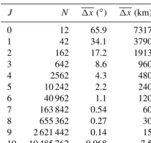
Table 1. Hierarchy of multiscale primal (triangle) grids derived by edge bisection from the icosahedron at scaleJ=0.N=10× 4J+2 is the number of computational elements (lozenges),1x= (4/
√
34π2a2/20/4J)1/2 is the average triangle edge length on Earth. Each computational element is made up of one node (for scalars), three edges (for velocities) and two triangles (circulation). Therefore, the total number of data elements is 5Nper vertical level. Note that there are two exceptional points to deal with the poles when the icosahedron is unfolded into 10 lozenges. Typically, the coarsest (optimized) level is 4≤J≤9 with three to five levels of refinement.
J N 1x(◦) 1x(km)
0 12 65.9 7317
1 42 34.1 3790
2 162 17.2 1913
3 642 8.6 960
4 2562 4.3 480
5 10 242 2.2 240
6 40 962 1.1 120
7 163 842 0.54 60
8 655 362 0.27 30
9 2 621 442 0.14 15
10 10 485 762 0.068 7.5
et al. (2013). As an alternative, we can also use the grid op-timization proposed by Xu (2006), although it produces less optimal grids.
A more fundamental challenge particular to this adaptive flux-based method on staggered grids is that the dual hexag-onal grids on two successive scales are no longer nested as they are on the plane. This means that we must keep track of the various configurations of small overlapping hexagons when computing the flux restriction (see Sect. 4.3 and Fig. 4 of Aechtner et al., 2015, for more details). Note that the pri-mal grid of triangles remains nested on the sphere, which means that the restrictions of velocity, Bernoulli and circula-tion are straightforward.
2.3 Parallelization and data structure
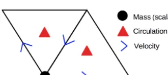
The parallelization and data structure must take account both the icosahedral geometry and topology of the spherical dis-cretization and the fact that the grid is adaptive and mul-tiscale. The C grid is stored as a regular data structure by grouping one node (mass and other scalars), two triangles (circulations) and three edges (velocities) into one computa-tional element, a “lozenge” as shown in Fig. 3. The icosahe-dron is composed of 20 triangles grouped into 10 lozenges. Therefore, a grid resulting from refining an icosahedron can be divided into 10 subgrids, each of which can be stored and accessed in a regular fashion. Note that at the edges of the lozenges the two adjacent regular grids of the origi-nal icosahedron are rotated with respect to each other. This is dealt with by surrounding the 10 lozenge subdomains by
ghost/halo cells. The halo cells are also used for parallel com-munication during boundary updates between cores.
The most natural way to store two-dimensional data with a dyadic multiscale structure is to use a quad tree, where each branching represents a new finer scale. However, in an adap-tive method, some branches are pruned and accessing neigh-bours would require wasteful traversing of the tree structure. We decided to use a hybrid data structure where each quad tree terminates in a patch. The patches are small 4×4 or 8×8 regular grids. This structure reduces the number of lev-els in the quad tree and makes it more computationally effi-cient to find neighbours. A similar hybrid approach was used by Behrens (2009) and Hejazialhosseini et al. (2010). Using patches increases memory slightly because inactive elements are stored. It is also possible to try to optimize the patch size for best computational performance for a particular problem, although 8×8 appears optimal in most cases. Note that the patches do not affect the results of the computation; they just improve computational efficiency.
The domain decomposition used for parallelizing the com-putation is based on distributing the lozenge subdomains on the coarsest levelJmin(and their associated children) to dif-ferent cores. Each core can compute several subdomains and having several small subdomains per core can improve cache efficiency. Note that there are 10×4Jmin−(P+1)subdomains at the coarsest level with a patch size of 2P×2P. For example, ifJmin=7 andP =2, the coarsest scale containsND=2560 subdomains. Because the number of coresNcore≤ND, large numbers of cores are usable only by largeJmin.
Figure 2.Wavelet transform on a non-adaptive icosahedral grid with three scales.
Figure 3. Lozenge: basic computational element containing one node (for mass and other scalars), three edges (for velocities) and two triangles (for circulation). Separate wavelet transforms are pro-vided for the nodes (scalar valued) and edges (vector valued). The adaptive grid consists of the significant nodes and edges, together with nearest neighbours in position and scale necessary for dynam-ics.
Every subdomain is extended to hold as many ghost/halo cells as necessary for the various required operators. The values at the halo cells are communicated as needed. Intra-core communication is done by copying and inter-Intra-core com-munication is done using mpi. During grid adaption, new patches are added and removed as required and grid con-nectivity between domains is updated (via mpi as neces-sary). Critical communications are carried out locally point to point rather than using global communication where possi-ble. Where possible, communication is non-blocking so that the computations can continue while communication is tak-ing place in the background.
This parallelization algorithm is reasonably efficient for at least several hundred or a few thousand cores. Dubos and Kevlahan (2013) found that good weak parallel efficiency is possible with as few as 1300 computational elements per core in adaptive runs. The three-dimensional code has better parallel efficiency because the column structure of the data produces a higher computational load for each active grid el-ement. We present some representative strong and weak par-allel scaling results in Sect. 5.1.
3 Hydrostatic dynamical equations and ALE vertical coordinates
As mentioned in the introduction, we use thedynamico discretization of the three-dimensional hydrostatic multilayer shallow water equations (Dubos et al., 2015) in compressible form. The discrete dynamical equations are derived from the discrete Hamiltonian, which allows the construction of en-ergy or potential enstrophy conserving equations. The prog-nostic variables aremik (mass),2ik (mass-weighted
poten-tial temperature) andvek(velocity), whereklabels a full
ver-tical level,lan interface (half level) between full vertical lev-els,ian hexagonal or pentagonal cell,va triangle andean edge. In terms of the Hamiltonian, their evolution equations are
∂mik
∂t +δi ∂H ∂vek
=0, ∂2ik ∂t +δi
θek∗ ∂H
∂vek
=0, (7) ∂vek
∂t + f
v+δvvk
mikv
∂H ∂vek
potential vorticity ⊥
+δe
∂H ∂mik
Bernoulli +θek∗δe
∂H ∂2ik
Exner =0,
(8) whereδi,δeandδvare discrete divergence, gradient and curl
operators yielding values at cells, edges and triangles, respec-tively,fvis the Coriolis parameter, andθek∗,mikvare values
ofθandmreconstructed at edges and triangles, respectively, by appropriate averaging. Indices than can be inferred may be omitted, as inδvvk≡δvvek. Evaluating the Hamiltonian
∂µik
∂t +δiUk=0, (9)
∂2ik
∂t +δi(θ ∗
ekUk)=0, (10)
∂vek
∂t +δeBk+θ ∗
ekδeπk+(qkUk)⊥e =0, (11)
whereµik=ρik1zik, and we have assumed Lagrangian
ver-tical coordinates (so the verver-tical mass fluxes are not present). Potential temperature θik=2ik/µik and θek=θik
e
.µik is
a pseudo mass density (equivalent to ρik1zik),Uek is the
horizontal mass flux, Bik is the Bernoulli function, πik=
π(αik, θik)is the Exner function,αik is the specific volume,
andqvkis the potential vorticity. In the compressible case we
consider here, the Bernoulli function is given by Bik=Kik+8il
k
, (12)
where Kik is the discrete kinetic energy computed from
u2ek using appropriate averaging, and 8il is the
geopoten-tial at vertical layer interfaces l. The discrete operators δi
(divergence with result at a node), δe (gradient with result
at an edge) and (·)⊥ (perpendicular flux) are defined as in Ringler et al. (2010) and the shallow water equation version ofwavetrisk.
Each evaluation of the trend requires integrating vertically down to find the surface pressure and then integrating up to find the Exner function and geopotential (and hence the Bernoulli function).
The choice of Lagrangian vertical coordinates (rather than mass based) is simple, computationally efficient and espe-cially well suited for ocean modelling since it virtually elim-inates numerical vertical diapycnal diffusion, unlike az co-ordinate. This will become important when we develop the ocean version of wavetrisk(see Kevlahan et al., 2015). The vertical coordinates are pressure based and may either be evenly spaced or hybrid (σ). As the flow develops, the vertical levels expand and contract, which can lead to loss of accuracy or even negative mass (if a layer collapses to zero thickness). To avoid this problem, we remap the vertical co-ordinates back to the original coco-ordinates either every time step or every 10 time steps or so. The remapping takes about 7 % of CPU time if done every time step.
Remapping Lagrangian vertical coordinates is a common technique in ocean modelling (e.g. Petersen et al., 2015), where the target grid is updated at each time step to optimize numerical accuracy and stability (e.g. the target grid may be based on approximately isopycnal or isentropic coordinates) and is referred to as an ALE coordinate system. Optimiz-ing the target grid inwavetriskwould add a sort of verti-calradaptivity in addition to the wavelet-based horizontalh adaptivity, where the number of vertical levels would remain constant but their locations would be chosen optimally. For example, Kavcic and Thuburn (2018) choose the target grid
levels at each time step to keep the vertical levels close to isentropic. This requires solving a small elliptic optimization problem at each grid level. In principle, it is also possible to include verticalhadaptivity by locally de-activating certain vertical layers if the vertical interpolation errors are small. We have testedwavetriskwith a variety of piecewise con-stant, piecewise linear, piecewise parabolic and piecewise quartic remapping schemes, modified from packages sup-plied by Shchepetkin (2001) and Engwirda and Kelley (2016, https://github.com/dengwirda/PPR, last access: 25 Novem-ber 2019). The user can select no limiter, a monotone limiter or a weighted essentially non-oscillatory (WENO) limiter. Any of these remapping algorithms can be selected simply by changing a parameter.
Mass densityµ, potential temperatureθ and velocitiesu, v,w are remapped onto the original hybrid pressure coor-dinates. This remapping scheme conserves mass, potential temperature and divergence and appears to perform well. We also tested Lin (2004)’s scheme, which remaps momentum and total energy, but it proved to be less stable.
We found that simple piecewise constant remapping gives qualitatively incorrect results for zonally averaged statistics in the Held and Suarez (1994) test case, but that it is sufficient for the mountainduced Rossby wave and baroclinic in-stability test cases. Piecewise linear and piecewise parabolic remapping give qualitatively accurate results. The target grid could be optimized at each remap, as in ocean models and as explored by Kavcic and Thuburn (2018) for theendgame general circulation model (GCM). However, the current pro-cedure gives good results in the test cases we have examined. The dynamical equations are advanced in time using the fourth-order four-stage low-storage Runge–Kutta rou-tine used indynamico(Dubos et al., 2015). Various strong stability-preserving schemes (e.g. the third-order three-stage scheme RK33ssp, RK45ssp) are also available as options (Spiteri and Ruuth, 2002).
In many cases, the code runs stably without any additional diffusion or filtering of small scales. However, in rare cases, the code crashes due to numerical instability. In order to im-prove stability, a regular or second-order hyperdiffusion term is added to the dynamical equations for the prognostic vari-ables to damp the largest wavenumbers (both the divergent and vortical modes of the momentum equation are damped). Using the discrete operator notation of Dubos et al. (2015), the diffusion terms for scalars, divergence and vorticity are, respectively,
Dφ=Kφδi l e de δe φ Ai , (13)
Dδ=Kδδe 1 Ai δi l e ld ve , (14)
Dω=Kωδe 1
Av
δv(ve)
where de is a triangle edge length (primal grid), le is a
hexagon edge length (dual grid),Aiis a hexagon area,Avis a
triangle area. These discretizations correspond to the contin-uous differential operators∇ ·∇(φ),∇(∇ ·u)and∇ ×(∇ ×u), respectively.
A generalpth-order hyperdiffusion operator is defined as an iterated Laplacian operator1pcorresponding toDpφ,Dδp, Dωp. We choose eitherp=1 (regular diffusion) orp=2
hy-perdiffusion. Diffusion may be applied at each time step or everyNdiff>1 time steps (whereNdiffis limited by viscous stability in time). The diffusion coefficient K is chosen to give the same amount of damping over a time step:
K=1x 2p
1t CNdiff, (16)
where1x=(4π a2/(10 4J+2))1/2is the average grid scale and C is an empirical constant chosen to ensure stability, which may be different for different variables.
Note that in addition to ensuring stability, adding diffu-sion can improve the efficiency of the adaptivity by damping out small fluctuations that might otherwise produce some lo-cal grid refinement. This effect is especially significant when adapting on the wavelets of the tendencies. We present results both with and without explicit diffusion.
4 Adaptivity
To extend the adaptive algorithm for the two-dimensional shallow water equations reviewed in Sect. 2.1 to the three-dimensional case, we simply apply the two-three-dimensional al-gorithm to each vertical layer in turn and then define the adapted grid to be the union of the adapted grids over all vertical layersk=1, . . ., N.
After the time step and vertical regridding have been com-pleted, the wavelet transforms of mass density µ, mass-weighted potential temperature2and velocityuare calcu-lated for each vertical level. Then, grid points are labelled active if their associated wavelet coefficient has a magni-tude greater than or equal to the appropriate relative error threshold. Nearest neighbours are added to the adjacent zone in position and scale. Note that a node is labelled active if any of its associated scalar wavelets (i.e. mass wavelet or mass-weighted potential temperature wavelet) is significant in any vertical layer. An edge is labelled active if its asso-ciated vector wavelet (i.e. velocity wavelet) is active in any vertical layer. Grid points are added as necessary to satisfy the perfect reconstruction criterion (so the grid points neces-sary to compute the wavelet coefficients are present). Finally, grid points required for the TRiSK operators are labelled. An inverse wavelet transform interpolates the solution conserva-tively onto the new adapted grid. The adaptivity algorithm is summarized in Algorithm 1.
The adaptive algorithm produces an adapted grid consist-ing of vertical columns of varyconsist-ing horizontal size. In practice, a maximum scaleJis usually set based on available compu-tational resources and user requirements. This “column adap-tivity” approach is not optimal for vertically tilted structures, but it provides much better load balancing and is far sim-pler than dealing with fully three-dimensional adaptivity. In addition, we can take advantage of an ALE formulation for the vertical coordinate which is often more flexible and ac-curate than az-coordinate system. We show in the results section that column adaptivity provides accurate results and good grid compression ratios. Note that the vertical grid is remapped (if necessary) before adapting the horizontal grid. The normalizations for the absolute tolerances εµ=
are determined dynamically by calculating the appropriate norms separately for each vertical layer at each time step.
The choice of normalization for the absolute thresholds εµ,ε2andεuis a crucial and sensitive part of the algorithm
since they guarantee the relative accuracy and efficiency of the method. In the shallow water case, we determined the tol-erances for mass and velocity based on dimensional analysis of the tendencies in the inertia–gravity and quasi-geostrophic regimes. This sort of dimensional analysis is not feasible for the three-dimensional equations, so we have developed two strategies to ensure uniform control of the relative error in the tendencies of the prognostic variables in each vertical layer.
As we mentioned earlier, in the first approach, these tol-erances are set by dimensional analysis using a knowledge of the appropriate scales for the test problem under consider-ation. This gives reasonable results for problems with fairly stationary evolution but can lead to less accurate results if the dynamics change significantly during the course of the sim-ulation. It also generally means that the tolerances are set to the same value for all vertical levels.
In the second approach, the relevant norms are calculated dynamically at each time step and at each vertical level to en-sure they are consistent with the actual state of the flow. This approach is more generally applicable and does not require the user to have any a priori knowledge of the solution.
In addition to determining how to calculate the normaliza-tion for the thresholds, we also need to decide which wavelets we are filtering. In the shallow water case, we always directly filtered the wavelets of the solution, which measure the inter-polation errors of the variables themselves between two grid levels at a given time step. Although this does not directly control the tendency error, analysis of a linearized problem suggests that it should provide some control of the tendency error provided the solution is smooth.
Consider a set of n coupled linear ordinary differential equations:
du
dt =A(u),u(0)=u0, (17)
whereAis an(n×n)constant coefficient matrix. Applying an Euler scheme gives the time stepun+1=un+1tAun. The
error (wavelet coefficient)eunsatisfies the same equation, so we have
eu
n+1=(I+1tA) eu
n,
||eun+1||
||un|| ≤(1+1t||A||)
||eun||
||un||,
where Iis the identity matrix and we have used the trian-gle inequality. Now, if we assume that ||
eu
n||/||un|| ≤ε by
wavelet filtering ofun, we have the following bound on the relative error:
|| eu
n+1||
||un|| ≤ε(1+1t||A||). (18)
If A is symmetric, then||A||2=ρ(A), where ρ(A) is the spectral radius of A (largest magnitude eigenvalue of A, |λ|max). Thus, we have that
|| eu
n+1|| 2 ||un||
2
≤ε(1+1t ρ(A)). (19)
However, a necessary condition for stability of the Euler method is that
1t ρ(A)≤2, (20)
which gives ||
eu n+1||
2 ||un||
2
≤3ε. (21)
We have therefore shown that wavelet filtering of the solution itself provides control of the relative error of the solution over one time step for symmetric discretizations. In general, for non-symmetricA, we have
|| eu
n+1|| 2 ||un||
2
≤ε(1+1t σ (A)), (22)
whereσ (A)is the largest singular value ofA. However, there exists an >0 such that ||A|| ≤ρ(A)+ for any matrix norm|| · ||. Thus, we can expect similar relation to Eq. (21) to hold for more non-symmetric discretizations. Although we have only considered the linear constant coefficient case, the results suggest that dynamic wavelet filtering of the solution, together with dynamic calculation of the normalization of the thresholds, should control the relative error of the solution over one time step.
Now, consider filtering on the wavelets of the tendenciesT themselves at the previous time step so that||eT
n
||/||Tn|| ≤ ε, whereeT is now the error (wavelet coefficient) of the ten-dency. To first order in1t, we have
e
Tn+1=eT n
+1t (JT(eu n, tn)
e Tn+∂T
∂t (eu
n, tn)), (23)
whereJT(eu
n, tn)is the Jacobian matrix of the tendency
eval-uated at the previous time step. In the case of an Euler method applied to a linear constant coefficient system of ordinary dif-ferential equations as we considered above, we haveT =Au and the errors in the tendencyTe(wavelets of the tendency) satisfy
e
Tn+1=(I+A)eT n
,
||eT n+1
|| ≤ ||eT n
|| + ||ATen||, ||eT
n+1 || ≤ ||eT
n
|| + ||A||||eTn||,
where we have used the triangle and Schwartz inequalities. Normalizing by||Tn||and recalling that wavelet filtering en-sures that||eT
n
||/||Tn|| ≤εgives the result ||eT
n+1 ||
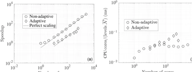
Figure 4.Strong scaling ofwavetriskon the Compute Canada machineniagarafor a simulation of the Held and Suarez (1994) general circulation experiment for a perfectly balanced (non-adaptive) run at a resolution ofJ=8 (1/4◦) and for a strongly unbalanced (dynamically adaptive) run at a maximum resolution ofJ=9 (1/8◦) resolution with trend-based error toleranceε=0.08.(a)Speedup compared with perfect (linear) scaling. The non-adaptive case has perfect linear scaling for more than eight cores, while the adaptive case has power law scaling of approximately 0.78.(b)Absolute strong scaling performance in milliseconds (ms) (wall-clock time per time step multiplied by the number of cores, i.e. CPU hours per time step, divided by the average number of active nodes over all vertical levels and all scales).Nis the average number of active nodes over all scales. Note that the absolute times shown in panel(b)are slower than equivalent times reported in Table 2 because we used a RK45ssp (with one additional trend evaluation) and code was compiled withgfortranrather thanifortfor the scaling runs.
Again, ifAis symmetric, we have||A||2=ρ(A), and using ρ(A) <1/1tfor the Euler method we find
||eT n+1
||
||Tn|| ≤
1+ 1 1t
ε≤Cε. (25)
Inequality (25) shows that filtering the wavelets of the ten-dencieseT
n
from the previous time step effectively controls the relative tendency error in the next time step up to a con-stant factor depending on the discretized system. Note that filtering the wavelets of the tendencies is slightly more ex-pensive since it requires an additional evaluation of the ten-dencies (or an additional inverse wavelet transform).
In the following section, we applywavetriskto solve three standard test problems for hydrostatic dynamical cores. The emphasis is on evaluating the adaptivity in the three-dimensional hydrostatic version, rather the basic accuracy of the method since the underlying discretization is the same as dynamicoand we have already assessed the basic features of the error control in previous work on the shallow water equations. We directly compare the options of nonlinear fil-tering the wavelets of the solution and wavelet filfil-tering the wavelets of the tendencies. Filtering the tendencies is more precise but more sensitive to the choice of threshold.
5 Validation test case results
5.1 Parallel and computational efficiency
The adaptive wavetrisk code has significant computa-tional overhead compared todynamico, which solves the same discretized equations. This overhead is required to deal with the local geometry of the grid (which is not
preputed), the multiscale grid structure and the parallel com-munication on the hybrid data structure. This overhead in-creases with the number of refinement levels and dein-creases for larger patch sizes. A lower bound on the overhead can be estimated by directly comparing wall-clock time for wavetriskanddynamicosince both codes are based on the same TRiSK discretization. The codes solved Dynami-cal Core Model Intercomparison Project (DCMIP) 2008 test case 8 (see Sect. 5.2) on the uniform grid J =6 (1◦ de-gree) with 27 Lagrangian vertical levels and 8×8 patches for wavetrisk. The codes were run on 160 cores. This limited test suggests that wavetrisk is approximately 50 % slower thandynamicoper active grid point. The ac-tual overhead depends on the number of refinement levels and the patch size (larger patch sizes are more computational efficient but limit the number of cores and increase mem-ory overhead). Note thatdynamicousually runs with mass-based vertical coordinates, which adds an additional 15 % to its CPU time.
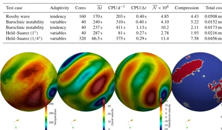
Figure 5.Adaptive Held and Suarez (1994) general circulation experiment att=500 h with maximum resolution of 1/8◦used for the strong parallel scaling results shown in Fig. 4. Results are shown at the vertical level corresponding to 850 hPa. The rightmost figure is the adaptive grid with a grid compression ratio of about 4.5.
of the cost, so remapping every 10 time steps decreases the overhead difference to about a factor of 3.7. Using RK33ssp instead of RK4 further reduces the overhead to about a factor of 2.8. Note that, unlikedynamico, we have not made a se-rious effort to optimize the performance ofwavetriskand it is certainly possible to reduce this overhead significantly. Nevertheless, we will show that compression ratios of up to 1000 times are achievable using the adaptive code and it is certainly much faster than the equivalent non-adaptive code for high-resolution intermittent problems.
In order to estimate strong parallel scaling performance, we ran two Held and Suarez (1994) general circulation ex-periments. The first run was non-adaptive at horizontal res-olution 1/4◦with 30 vertical levels for 10 time steps. This case is balanced and Fig. 4a shows that it has linear speedup from about 8 to at least 2560 cores (the lack of linear scaling for four or fewer cores is due to the intrinsic overhead of par-allel computations). Although speedup is a commonly used measure of parallel scaling, a more sensitive measure is CPU time per time step divided by the number of vertical columns per core. Perfect scaling is then a constant, and its value gives an indication of absolute performance. Figure 4b shows that this measure is indeed approximately constant from 4 to 2560 cores.
The second trial was fully adaptive using trend filtering, with a minimum horizontal resolution of 1/2◦and three lev-els of refinement to 1/8◦ and 18 vertical levels computed with a relative error toleranceε=0.08. This simulation was first run for 500 h to allow the climate dynamics to develop. Figure 5 shows the solution and adaptive grid at t=500 h. The grid compression ratio is a relatively modest 4.5. The simulation was then restarted and run for another 4 h (about 300 time steps) to estimate strong parallel scaling and tim-ing. The computational load was rebalanced on restart, but there was no further rebalancing. The load imbalance (ratio
of highest to average load) varied from 3 to 8 during this sim-ulation. This run therefore represents a very unbalanced case. Nevertheless, Fig. 4a shows close to linear speedup (power law exponent of 0.78) to at least 640 cores. The more precise measure of strong scaling in Fig. 4b is further from a constant (with a maximum variation of 3 times), although there is not a definite trend with increasing numbers of cores. Since weak scaling performance is a better indication of parallel perfor-mance than the strong scaling, these results suggest weak scaling should be good to much larger numbers of cores. In fact, the shallow water code on whichwavetriskis based showed 70 % weak scaling efficiency for as few as 1300 com-putational elements per core (Aechtner et al., 2015). The cur-rent three-dimensional code has better parallel performance since the subdomains are distributed to the cores as complete vertical columns, which means each core has a larger load.
Table 2. Summary of actual computational performance for each of the test cases considered here. All runs were done on the Compute Canada machineniagaraand the values shown are averages over the whole simulation. CPU is wall-clock time,Nis the average number of active nodes (over all vertical levels and all scales), total cost is wall-clock time per time step multiplied by the number of cores (i.e. CPU hours per time step) per active node per vertical level. (Note that total cost does not take into account the speedup due to parallelism or adaptivity: it measures CPU hours per active node.) The Rossby wave run is more expensive because it uses a smaller patch size (4×4 rather than 8×8) in order to run on 160 cores withJmin=5. Please see the discussion at the beginning of Sect. 5.1 for an explanation of the trade-offs involved in patch size versus number of domains.
Test case Adaptivity Cores 1t CPU d−1 CPU/1t N×104 Compression Total cost
Rossby wave tendency 160 170 s 203 s 0.40 s 4.85 4.43 0.0508 ms
Baroclinic instability variables 40 240 s 310 s 0.40 s 4.10 5.22 0.0152 ms Baroclinic instability tendency 40 237 s 411 s 1.13 s 10.2 2.11 0.0173 ms
Held–Suarez (1◦) variables 40 287 s 81 s 0.27 s 2.78 1.93 0.0216 ms
Held–Suarez (1/4◦) variables 320 66.5 s 375 s 0.29 s 11.4 7.58 0.0456 ms
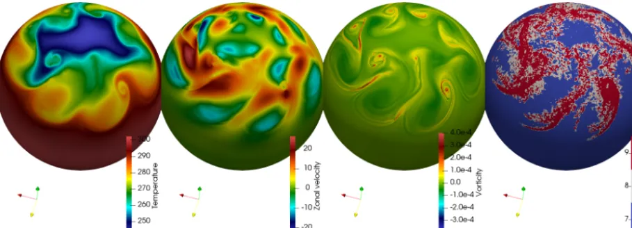
Figure 6.Results of the adaptive simulation of the mountain-induced Rossby wave case shown at 700 hPa at day 25.
5.2 DCMIP 2008 test case 5: mountain-induced Rossby wave train
The first validation we consider is the mountain-induced Rossby wave train used in DCMIP in 2008 (Jablonowski et al., 2008). This test case is relatively smooth and does not produce much small-scale structure. It is, however, a good test of the ability of the adaptive algorithm to track develop-ing wave instabilities. It is similar to the case described in Tomita and Sato (2004) but with a hydrostatic surface pres-sure. The simulation starts from smooth, balanced isothermal initial conditions and a Rossby wave train instability is gen-erated by an isolated Gaussian mountain over the course of the first 15 days.
The coarsest scale in the simulation is J=5 (2◦) and the finest scale is J=7 (1/2◦) with 27 vertical hybrid σ -pressure levels. The vertical grid is remapped when the thick-ness of a vertical level has dropped to 30 % of its initial value. There is no diffusion. The grid is adapted on the tendency wavelets. We run the simulation for a total of 30 days. The results are shown at day 25 on the sphere in Fig. 6.
Figure 7 shows equidistant cylindrical rectangular latitude–longitude projections of the results of the adaptive simulation at 700 hPa at day 25. The adaptive data are first interpolated to a uniform J=7 (1/2◦) grid, then interpo-lated to the desired pressure level and finally projected onto the plane. The results are in good qualitative agreement with those shown in the DCMIP 2008 report (Jablonowski et al., 2008). There is some difference in the weaker structures, which is inevitable given that the adaptive simulation neces-sarily resolves the more intense structures more highly than the weaker ones.
Figure 7.Latitude–longitude projections at 700 hPa of the adaptive simulation of the mountain-induced Rossby wave test case at day 25.
5.3 DCMIP 2012 test case 4: baroclinic instability of jet stream
Jablonowski and Williamson (2006) proposed a deterministic test case for dry dynamical cores of atmospheric general cir-culation models that simulates the evolution of a baroclinic wave in the Northern Hemisphere. Perturbation of an ana-lytic steady state solution triggers a baroclinic instability that generates a series of vortices. These vortices grow and in-teract, eventually producing a two-dimensional turbulence-like vorticity field of intense filaments and vortex cores. The rapid development of the vortical instability and its subse-quent evolution is a challenging case for an adaptive method. This baroclinic instability was test case 4 of DCMIP 2012.
With a sufficiently low relative tolerance (e.g. ε=0.03 when adapting on the solution), wavetrisksuccessfully captures the explosive cyclogenesis around day 8 and subse-quent breaking of the wave train around day 12 to produce a series of intense filamentary vortices (see Sect. 10). This calculation uses quadratic piecewise parabolic remapping at each time step Engwirda and Kelley (2016, https://github. com/dengwirda/PPR, last access: 25 November 2019).
Figure 8 shows the surface pressure and temperature at day 9, which agree reasonably well with the equivalent re-sults in Fig. 6 from Jablonowski and Williamson (2006). Note that we do not expect exact agreement since the adap-tive simulation does not resolve all regions uniformly. Be-yond day 12, the vortices interact to produce turbulence-like flow in both hemispheres. These results therefore validate the ability of the model to capture suddenly developing instabil-ities and track their evolution to a turbulence-like state.
Next, we compare the characteristics of the solution-filtered and trend-solution-filtered variants of wavetrisk. In both cases, the maximum scale isJ=7 (1/2◦) and we use 27 ver-tical hybridσpressure levels as specified in Jablonowski and
Figure 8.Latitude–longitude projections of surface pressure and temperature at vertical level 4 (about 867 hPa) of the adaptive sim-ulation of the baroclinic instability test case at day 9.
Williamson (2006). There is no explicit diffusion added to stabilize the dynamics or to damp out grid-scale oscillations and both simulations using RK45ssp time integration (Spiteri and Ruuth, 2002). It is important to note that, although this is a deterministic test case when simulated non-adaptively, adaptivity necessarily neglects some less dynamically impor-tant structures and so the details of flows with different tol-erances eventually diverge once they become turbulent (after roughly 12 days). This is, however, an optimal test case for adaptive methods, since at early times, only a small portion of the flow is active, which allows high compression ratios. In fact, until the instability develops, a very coarse grid and large time step are sufficient.
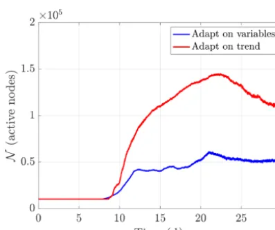
com-Figure 9.Comparison of the number of active nodesNfor the baro-clinic instability when adapting on the trend or adapting on the solu-tion. The relative error threshold was set toε=0.04 when adapting on the solution and ε=2.6 when adapting on the trend. In both cases, the active scales arej=5,6,7 and there is no additional dif-fusion. The tolerances were set to achieve similar compression ra-tios at 9 days. The total number of available grid points is 8.6×10⁵, and so the minimum grid compression ratio is 3.6 when adapting on the solution and 1.5 when adapting on the trend. The average com-pression ratio is 5.2 when adapting on the solution and 2.1 when adapting on the trend.
pression ratios at day 9 and were set based on dimensional analysis (i.e. they are fixed in time). Both options use similar numbers of grid points until about day 12 when the flow be-comes more turbulent. Once the flow is turbulent, adapting on the trend uses significantly more grid points. Although the number of grid points used by both options is similar un-til day 12, the methods distribute the same number of grid points quite differently.
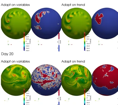
Figure 10 compares the vorticity fields and active grids at days 9 and 20. At day 9, adapting on the solution distributes the available grid points to track all the developing vortices. In contrast, adapting on the trend concentrates all grid points on the two strongest vortices. In addition, the peak vorticity when adapting on the solution, 5.2×10⁻⁴s−1, is higher than when adapting on the trend, 1.9×10⁻⁴s−1. Once the flow is turbulent, at day 20, adapting on the trend uses about 2.8 times more grid points than adapting on the solution.
Adapting on the solution appears to be more efficient since adapting on the trend is sensitive to grid-scale noise in the trend (the solution is smoother than the trend). Adapting on the trend uses fewer overall grid points when the tolerances are rescaled dynamically (i.e. when the trend norms are re-computed at each time step), but the resulting adapted grid is quite sensitive to local fluctuations in the trend. This ef-fect is much less pronounced when diffusion is added. Based on this and other examples we have investigated, adapting on the solution appears to be preferable when there is little or no diffusion added to damp out grid-scale noise.
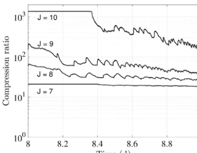
It is interesting to investigate how the grid compression ratios change as we increase the maximum allowed resolu-tion. The main advantage of adaptive methods is for inter-mittent problems that require very high local resolution not attainable using static grid methods. This requires that the grid compression ratio increases significantly with the maxi-mum allowed resolution. Figure 11 compares grid compres-sion ratios for four different maximum resolutions ranging fromJ=7 (1/2◦) toJ =10 (1/16◦) from day 8 to day 9 at the onset of the instability. The simulations have no diffusion and are adapted on the trends. Unsurprisingly, the compres-sion is very high at the onset of the instability at day 8, over 1300 atJ=10. At day 9, once the initial vortices have de-veloped, the compression ranges from about 20 atJ=7 to about 200 atJ =10. Note that we have found that we can also use a higher relative error threshold at higher resolutions which further increases the compression.
This scaling test suggests that the adaptive method should be especially advantageous at high maximum resolutions for vorticity-dominated flows. Although in this flow the insta-bility is highly localized, Aechtner et al. (2015) found com-pression ratios of about 20 for a homogeneous isotropic shal-low water turbulence case on the sphere with scales J= 5, . . .,10.
5.4 Held and Suarez general circulation experiment
Held and Suarez (1994) is a classic test case for dynamical cores of atmospheric general circulation models. It uses sim-plified “physics” (i.e. radiation and friction/drag models) that nevertheless produce realistic general circulation over rel-atively short timescales of O(102)days. For example, Liu and Schneider (2010) have used simple Held–Suarez-type physics to realistically model the general atmospheric circu-lation of Saturn. This model uses height-dependent Rayleigh damping to represent boundary-layer friction and a height-and latitude-dependent Newton cooling relaxation of poten-tial temperature to a prescribed radiative–convective equi-librium. The temperature relaxation includes parameters ac-counting for cooling at the surface and top of the atmosphere as well as a tropopause. The Held–Suarez general circula-tion experiment adds a qualitatively new aspect to the Rossby wave and baroclinic instability tests we considered above: it includes physics source terms for the temperature and mo-mentum equations. None of the previous simulations have included these sorts of physics terms, either in three dimen-sions or in two dimendimen-sions on the sphere or on the plane. Nevertheless, we expect the grid adaptation to track the ef-fect of the source terms either directly through their efef-fect on the trend or indirectly through their effect on the prognostic variables.
Figure 10.Comparison at days 9 and 20 of the grid compression ratios for the baroclinic instability when adapting on the trend or adapting on the solution. The relative error threshold was set toε=0.04 (fixed) when adapting on the solution andε=2.6 when adapting on the trend. In both cases, the resolution isj=5,6,7 and there is no additional diffusion. The tolerances were set to achieve similar compression ratios at 9 days. The vorticity field is shown at hybrid vertical level 4 (about 870 hPa).
low-resolution run has coarsest scaleJmin=4 and finest res-olutionJ=6 (about 120 km or 1◦) with toleranceε=0.04. The high-resolution run has coarsest scaleJmin=6 and finest resolution J=8 (about 30 km or 1/4◦) with toleranceε= 0.02. The low-resolution case is run on 40 cores and the high-resolution case is run on 320 cores. As in Wan et al. (2013), both cases start from the Jablonowski and Williamson (2006) zonally symmetric initial condition with random noise of magnitude 1 m s−1added to the zonal wind. In both cases, the simulations are first run non-adaptively for 200 days at the coarsest resolution and then restarted adaptively with the maximum resolution. The time step is adaptive with that of the CFL criterion. The maximum possible grid compression ratio for both cases is 21.
We use 19 vertical σ-pressure levels concentrated at the top and bottom of the atmosphere. The vertical grid is
remapped using a piecewise parabolic method with WENO limiting every 10 time steps.
Small-scale noise is damped with p=2 hyperdiffu-sion with diffuhyperdiffu-sion constantKφ=3.48×10¹⁵m4s−1,Kδ=
3.48×10¹⁶m4s−1andK
ω=2.17×10¹⁴m4s−1for the
low-resolution run and Kφ=2.33×10¹⁴m4s−1, Kδ=5.98×
1014m4s−1 andKω=1.46×10¹³m4s−1. The diffusion is
applied each time step in the main trend routine. The source terms for the potential temperature and the velocity repre-senting cooling and Rayleigh damping are implemented as a separate Euler step.
Figure 11.Grid compression ratios at the beginning of the baro-clinic instability for maximum resolutions J=7 (1/2◦), J=8 (1/4◦),J=9 (1/8◦) andJ=10 (1/16◦). In all cases, the coars-est resolution isJ=5 (2◦). The grids are adapted on the trend and there is no diffusion. Note that theJ=10 uses a higher relative er-ror thresholdε=4 than the others, which useε=2. Compression ratios increase significantly with increasing resolution, reaching as high as 200 times at day 9 for the maximum resolution case. Even at J=7, the code achieves a compression ratio of about 20 at day 9.
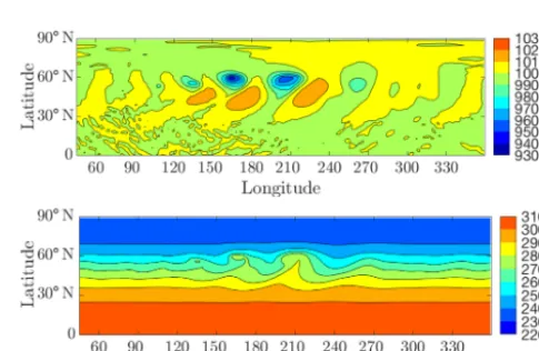
A typical low-resolution result is shown in Fig. 12 (top). The average grid compression ratio at this low resolution is only 1.9±0.1 withε=0.04. The adaptive algorithm is able to track the development and evolution of the fine-scale fil-amentary vortex structures over long times. Note that since the adapted grid is the union of adapted grids over all vertical levels, the adapted grid does not necessarily correspond ex-actly to the structures at the vertical level 11 (about 250 hPa) at the level of the upper atmosphere jets shown in the figure. Figure 13 shows standard first- and second-order statis-tics averaged zonally and over time for the low-resolution run. These statistics are qualitatively similar to those of Du-bos et al. (2015), Wan et al. (2013) and Lin (2004). (Lin, 2004 is the only one that uses Lagrangian vertical coordi-nates.) The main quantitative difference is in the slightly lower magnitude of the eddy kinetic energy. This difference is due partly to the use of Lagrangian vertical coordinates, where the remapping introduces additional dissipation, and partly to the additional dissipation generated by the adap-tivity at these relatively low resolutions. Lin (2004) did not show the eddy kinetic energy, but he reported a maximum variance of zonal wind of about 300 m2s−2, slightly larger than the 284 m2s−2we find here (not shown), and similar to the 301 m2s−2we find for the high-resolution case discussed below. Note that the original Held and Suarez (1994) paper did not present results for eddy kinetic energy.
The choice of remapping has a significant influence on the eddy kinetic energy. For example, we found that changing from a piecewise linear remapping to a piecewise parabolic remapping increases the maximum eddy kinetic energy by 53 m2s−2for a non-adaptive simulation with resolutionJ=
5 (240 km). Similarly, Lin (2004) found that including a monotonicity constraint in the remapping lowered the maxi-mum variance of the zonal velocity by about 20 m2s−2. We would also like to emphasize that piecewise constant remap-ping gives qualitatively incorrect results (e.g. zonal jets are too high), presumably because it is too dissipative and is not a good choice for this test case.
Larger tolerancesεeffectively increase dissipation, which decreases maximum eddy kinetic energy, while choosing a smaller tolerance leads to essentially no compression in the low-resolution run. (The other statistics are much less sensitive to ε.) Note that a fixed (non-adaptive) resolution Jmin=4 (4◦) gives a maximum eddy kinetic energy of only 280 m2s−2, much less than the published values of over 400 m2s−2at higher resolutions of 2 and 1◦. This suggests that the coarsest grid may be the main factor behind the lower eddy kinetic energy we observe here at higher compression ratios.
In contrast, Fig. 12 (bottom) shows typical results from the high-resolution simulation atε=0.02. The grid compression is clearly much higher than in the low-resolution run, and the fine scales are limited to a small neighbourhood of the high-intensity vorticity filaments. The average grid compression ratio for the high-resolution simulation is 7.6±0.5, exactly 4 times as large as in the low-resolution case. Both the com-pression and the fluctuations in the comcom-pression are much higher than in the low-resolution run. These results suggest that the adaptive method is useful primarily at higher reso-lutions and for more turbulent flows. This confirms our ear-lier observations for two-dimensional shallow water turbu-lence on the sphere (see Figs. 17 and 18 of Aechtner et al., 2015). The advantages of the adaptive method should be even greater for maximum resolutions higher thanJ=8 (1/4◦).
Figure 14 shows standard first- and second-order statis-tics averaged zonally and over time for the high-resolution run. The results are qualitatively very similar to the low-resolution run, with the main differences being more intense eddy momentum and eddy kinetic energy. The negative high-altitude zonal jet is also a bit stronger.
Figure 12.Typical results for the low-resolution (top) and high-resolution (bottom) Held and Suarez general circulation test case at 250 hPa. The grid is adapted on the solution with relative error toleranceε=0.04 in the low-resolution case andε=0.02 in the high-resolution case. The grid compression ratio is 2.0 for the low-resolution case and 7.5 for the high-resolution case.
6 Conclusions
This paper introduceswavetrisk: a new adaptive dynam-ical core.wavetriskuses the hydrostaticdynamico dis-cretization of Dubos et al. (2015) with a Lagrangian vertical coordinate. Second-generation discrete wavelet transforms provide control of the relative error of the solution in each vertical layer at each time step. The adaptive grid is uniform vertically and is composed of columns of varying horizon-tal sizes. In addition to the horizonhorizon-tal adaptivity, the vertical coordinates are remapped onto a hybrid σ-pressure coordi-nate using an arbitrary Lagrangian–Eulerian (ALE) scheme. In principle, ALE allowsradaptivity of the vertical coordi-nates by optimizing the target grid at each remap.h adaptiv-ity may also be possible in the future by deactivating some vertical layers (the so-called “dormant layers” used in ocean modelling).
The code is parallelized via domain decomposition us-ingmpiand the data are stored in a hybrid quad tree–patch data structure. The computational load is rebalanced at each checkpoint save. We demonstrate excellent strong parallel
scaling up to at least 2560 cores in the perfectly balanced case and close to linear scaling (exponent 0.78) up to at least 640 cores in an unbalanced case.wavetriskis 3– 4 times slower per active grid point than the non-adaptive dynamicocode, which suggests that we require a grid com-pression ratio of more than 4 for adaptivity to provide an ad-vantage in CPU time.
Figure 13.Time–zonal statistics for the low-resolution (Held and Suarez, 1994) test case with scalesJ=4,5,6 (maximum resolution of 1◦). The grid is adapted on the solution error with toleranceε=0.04. Statistics are averaged over 400 days after day 200 by interpolating saved data to the finest grid.
turbulent flow depends on the choice of error tolerance pa-rameter.
We have validated the code on three standard benchmarks: a mountain-induced Rossby wave train, baroclinic instabil-ity of a jet stream and the Held and Suarez general circu-lation experiment. These tests show thatwavetrisk cor-rectly captures the dynamics, including rapidly developing instabilities, with only a small portion of the total grid points available on a similar non-adaptive grid. The grid compres-sion ratio can reach over 200 in ideal cases (e.g. the start of the baroclinic instability with five levels of refinement) and is advantageous at sufficiently high resolutions even in more homogeneous flows like Held and Suarez.
Because adaptive climate simulation is a new field, we have deliberately included many options in our adaptive al-gorithm.wavetriskcan adapt on errors in the solution or on errors in the trend; it can run with no diffusion, Lapla-cian diffusion or hyperdiffusion. The vertical grid can be re-gridded (using a large selection of remapping schemes) each time step or only when a level becomes too narrow. And, of course, we can choose different relative tolerancesεand maximum and minimum grid resolutions. In many cases, the code is stable without diffusion and with grids adapted either on the solution or the trend. However, our test cases suggest that adapting on the solution (rather than the trend) generally gives more accurate and faster solutions for a given number of grid points. Including a small amount of diffusion stabi-lizes the code and reduces the number of active grid points by reducing grid-level noise.
It is clear that the main application of wavetrisk is for simulations at maximum resolutions unattainable by non-adaptive dynamical cores. In future work, we will use wavetriskto simulate simple Held–Suarez-type climates at much higher resolutions and for longer times and investi-gate the behaviour of more sophisticated physics parameter-izations in adaptive simulations. We are also developing an ocean variant ofwavetriskthat will improve the ALE for-mulation of the vertical coordinate and use penalization for bathymetry and coastlines. This work builds on the shallow water ocean model we presented in Kevlahan et al. (2015).
Code availability. WAVETRISK-1.0 is published under the Creative Commons 4.0 license at https://doi.org/10.5281/zenodo.3459710 (Kevlahan et al., 2019). The latest version of the code is WAVETRISK-1.1, which includes some bug fixes and two incompressible cases.
Author contributions. Both NKRK and TD have contributed to the research and paper preparation.
Competing interests. The authors declare that they have no conflict of interest.
Acknowledgements. Nicholas K.-R. Kevlahan would like to thank NSERC for Discovery Grant funding and Compute Canada for computing time and the Université Grenoble–Alpes and CNRS for visiting professorships. This work was supported by the French na-tional programme LEFE/INSU. The authors would like to thank Matthias Aechtner for his major contributions to the computational foundations ofwavetriskwhich are outlined in the papers on the shallow water equations version of the code on the sphere.
Review statement. This paper was edited by Paul Ullrich and re-viewed by two anonymous referees.
References
Aechtner, M., Kevlahan, N.-R., and Dubos, T.: A conserva-tive adapconserva-tive wavelet method for the shallow water equa-tions on the sphere, Q. J. Roy. Meteor. Soc., 141, 1712–1726, https://doi.org/10.1002/qj.2473, 2015.
Behrens, J.: Adaptive Atmospheric Modelling, Springer, 2009. Bryan, G. L., Norman, M. L., O’Shea, B. W., Abel, T., Wise, J. H.,
Turk, M. J., Reynolds, D. R., Collins, D. C., Wang, P., Skill-man, S. W., Smith, B., Harkness, R. P., Bordner, J., Kim, J.-h., Kuhlen, M., Xu, H., Goldbaum, N., Hummels, C., Kritsuk, An. G., Tasker, E., Skory, S., Simpson, C. M., Hahn, O., Oishi, J. S., So, G. C., Zhao, F., Cen, R., Li, Y., and Enzo Collaboration: ENZO: An Adaptive Mesh Refinement Code for Astrophysics, Astrophys. J. Suppl. S., 211, 19, https://doi.org/10.1088/0067-0049/211/2/19, 2014.
Chan, T., Golub, G., and LeVeque, R.: Algorithms for computing the sample variance: Analysis and recommendations, The Amer-ican Statistician, 37, 242–247, 1983.
Domingues, M. O., Gomes, S. M., Roussel, O., and Schneider, K.: An adaptive multiresolution scheme with local time step-ping for evolutionary PDEs, J. Comput. Phys., 227, 3758–3780, https://doi.org/10.1016/j.jcp.2007.11.046, 2008.
Dubos, T. and Kevlahan, N.-R.: Ann conservative adaptive wavelet method for the shallow water equations on staggered grids, Q. J. Roy. Meteor. Soc., 139, 1997–2020, 2013.
Dubos, T., Dubey, S., Tort, M., Mittal, R., Meurdesoif, Y., and Hour-din, F.: DYNAMICO-1.0, an icosahedral hydrostatic dynami-cal core designed for consistency and versatility, Geosci. Model Dev., 8, 3131–3150, https://doi.org/10.5194/gmd-8-3131-2015, 2015.
Engwirda, D. and Kelley, M.: A WENO-type slope-limiter for a family of piecewise polynomial methods, arXiv:1606.08188, 2016.
Ferguson, J.: Bridging Scales in 2- and 3-Dimensional Atmospheric Modeling with Adaptive Mesh Refinement, PhD thesis, Univer-sity of Michigan, 2018.
Ferguson, J., Jablonowski, C., Johansen, H., McCorquodale, P., Colella, P., and Ullrich, P.: Analyzing the Adaptive Mesh Re-finement (AMR) Characteristics of a High-Order 2D Cubed-Sphere Shallow-Water Model, Mon. Weather Rev., 144, 4641– 4666, https://doi.org/10.1175/MWR-D-16-0197.1, 2016. Harrison, E. J.: Three-Dimensional Numerical Simulations