COMPONENT MODE SYNTHESIS METHOD IN FEM BASED DYNAMIC ANALYSIS OF STRUCTURES

(1)

Available Online at www.ijpret.com 162

INTERNATIONAL JOURNAL OF PURE AND

APPLIED RESEARCH IN ENGINEERING AND

TECHNOLOGY

A PATH FOR HORIZING YOUR INNOVATIVE WORK

COMPONENT MODE SYNTHESIS METHOD IN FEM BASED DYNAMIC

ANALYSIS OF STRUCTURES

ROSHAN RAMDAS GADPAL

Deptt. of Applied Mechanics, Govt. Polytechnic Arvi , Dist Wardha

Accepted Date: 15/03/2016; Published Date: 01/05/2016

\

Abstract: Analyses in dynamics often require repeated operations, each involving the computational effort of a single static solution for a single load vector. To reduce the amount of computation it is helpful to reduce the size of matrices being manipulated. Reduction is accomplished by using a smaller set of degrees of freedom to represent the full set of degrees of freedom. The component mode synthesis method is a technique in finite element (FEM) analysis. This technique involves representing a system as an assemblage of components. In the system model, each component is represented in terms of its boundary and modal (generalized) degrees of freedom. Any loads applied at the interior of components need to be transferred to the boundary and generalized degrees of freedom. On the other hand, the response obtained is in terms of the boundary and vibration degrees of freedom of the component and needs to be transformed to obtain the response of the desired data recovery items. Thus component mode synthesis forms a reduced basis by assembling selected information from component substructures because design and control methods work best for the systems with a smaller number of degrees of freedom.

Keywords: FEM, Dynamic Analyses, D.O.F., Component Mode Synthesis.

.

Corresponding Author: MR. ROSHAN RAMDAS GADPAL

Access Online On:

www.ijpret.com

How to Cite This Article:

Roshan Ramdas Gadpal, IJPRET, 2016; Volume 4 (9): 162-171

(2)

INTRODUCTION

While performing dynamic analysis of structures using FEM, sometimes it becomes necessary to either to impose an elastic constraint or provide a reduced basis. A basis is a set of linearly independent vectors that can be combined in various proportions to represent or approximate other vectors. In view of structural vibration, other vectors imply the complete set of eigenvectors of FEM model. A basis is called reduced if it includes fewer vectors than the complete set.

Reduction can be accomplished by methods that range from intuitive to semi-rigorous. Few of the methods are Guyan reduction, Lanczos and subspace iteration methods, Response History Analysis using modal methods or Ritz vectors, Component mode synthesis method etc.

Component mode synthesis may be named as modal synthesis, substructuring synthesis and dynamic substructuring. The method is analogous to static substructuring , but dynamic substructuring does not preserve the full information content of the complete system. As in static analysis, motivations for use of component mode synthesis in dynamics are partly economic and partly managerial. Reduction order may be necessary for economical computation. Substructuring becomes all the more attractive when the structural form is repeated several times. After assembly of components, the reduced system can be used for the usual purposes of structural dynamics, that is, calculating frequencies and modes of the complete structure, response history analysis and so on.

Attachment d.o.f. are d.o.f. at nodes on lines or surfaces where substructure connected together. Component modes are vibration modes of individual substructures with their attachment d.o.f. fixed. Constraint modes are static displacement patterns of individual substructures produced by applying a unit displacement to each attachment d.o.f. in turn while all other attachment d.o.f. are kept fixed.

II. REVIEW OF LITERATURE

(3)

analysis. Furthermore, design and control methods work for systems with small number of d.o.f . To overcome these difficulties techniques for reduction of d.o.f. are required.

List of the publications is exhaustive and lot of literature on various methods of reduction of d.o.f. is available. There were two people who first felt the necessity of reduction of d.o.f in 1965. Guyan [1] and Irons [2] suggested that the relation between slaves (unwanted d.o.f) and masters (d.o.f. required to be retained in analysis) be dictated by stiffness coefficients. In 1973, Kidder [3] suggested that while performing Guyan Reduction, slave d.o.f. can be recovered after solving for masters. Shah V.N., et.al [4], 1982, Ong J.H. [5], 1987, Kim K. O., et.al. [6], 2001 discussed some numerical examples on reduced eigenvalue problem.

Response History Analysis can give the response (i.e. what are the accelerations, velocities and displacements of d.o.f. as functions of time) using Modal methods and related Ritz vector methods. In which, an alternative (and reduced) set of d.o.f. is solved as functions of time and then transformed back to the original physical d.o.f. If desired, the contribution to total response can be evaluated separately from the deformation response as reported by Craig R. R.[7] in his book on structural dynamics in 1981. He also reported Time-Domain and Frequency Domain Component Mode Synthesis Methods [8] in 1987.

In 1992, D. Hitchings [9] reported that there should be enough d.o.f. to represent the lowest vibration modes, as they are almost certain to be important. In 1994, Noor A. K. [10] enfocusssed on recent advances and applications of reduction methods. Shyu W.H. et.al.[11] presented a new Component Mode Synthesis Method: Quasi static Mode Compensation in 1997. Bertolini A.F. [12] reviewed eigensolution procedures for linear dynamic finite element analysis in 1998.

This paper summarize a component mode synthesis method, which is the method most widely used. To illustrate the method a numerical example has been solved and the results are compared with the standard results. This approach, along with the recommended check runs, has been shown to work successfully in this paper. The method is also shown to be extremely efficient.

(4)

In finite element analysis, a physical model of a structure with applied loads is represented mathematically as

M u’’ C u’ K u F t (1)

where M], C] and K] are the mass, stiffness and damping matrices, respectively.

u , u’ and u’’ represent the generalized displacements, velocities and accelerations at the physical degrees of freedom and F(t) represents the generalized forces at the physical degrees of freedom.

For an undamped free system, that is, in equations (1), C is assumed to be a null matrix and

F(t) is assumed to be a null vector. The eigenvectors so obtained are used to generate an eigenvalue problem of the form

([𝑲]_𝑪𝑴𝑺− 𝝎_𝒊𝟐 [𝑴]_𝑪𝑴𝑺 ) {𝒛′}𝒊 = {𝟎} …(2)

where, i is the mode number , [𝑲]_𝑪𝑴𝑺 & [𝑴]_𝑪𝑴𝑺 are the square size stiffness and mass matrices of the synthesized structure, and {𝒛′} is a vector of amplitudes of component modes and attachment d.o.f.

It is desired that the order of {𝒛′} be much less than the number of d.o.f. in original structure. Since, the constraints are imposed to obtain eqn. (2), it yields eigenvalues higher than corresponding eigenvalues of the original finite element structure for which all d.o.f. are obtained. Conceivably, all Ritz vectors used in obtaining the matrices of eqn. (2) are orthogonal to an eigenvector of the actual structure, in which case that mode will not be represented by eqn. (2). The possibility of missing an important lower mode will be minimized, if the number of component modes retained in analysis is increased.

Component modes of a typical substructure j are obtained by fixing all substructure attachment d.o.f. and solving the usual free vibrations we obtain,

([𝑲𝒏𝒏]𝒋− 𝝎𝒍𝟐 [𝑴𝒏𝒏]𝒋 ) {𝑫′}𝒋 = {𝟎}

[Φ]j = [D’1 D’2 D’3 … D’k]j …(3)

where suffix n is used to indicate those substructure d.o.f. that are not attachment d.o.f. suffix

l indicates a component mode and k is the number of modes retained in the modal matrix [Φ]j.

(5)

Constraint modes of substructure j are obtained by static analysis, using he stiffness matrix of the substructure with attachment d.o.f. included. Suffix a indicates attachment d.o.f., and suffix n indicates all other substructure d.o.f., which are regarded as internal d.o.f.

[ 𝐊𝑛𝑛 𝐊𝑛𝑎 𝐊𝑛𝑎𝐓 𝐊𝑎𝑎] 𝑗 [

𝛙

𝐈] j = [ 𝟎

𝐑] j …(4)

Here [I] is a unit matrix of size a x a and describes unit displacement of each attachment d.o.f. in turn while others are held fixed. For a unit displacement of mth attachment d.o.f., column m of [𝛙] is the resulting vector of internal d.o.f., and column m of [𝐑] is the resulting vector of reactions at attachment d.o.f. The upper partition of eqn. (4) yields

[𝛙]𝑗 = - [𝐊𝑛𝑛]_𝑗−1 [𝐊𝑛𝑎]𝑗 …(5)

The transformation between original d.o.f. { D }j of substructure j and substitute d.o.f. used

for synthesis is

{D }j ={𝐃_𝐃𝒏

𝒂} 𝒋 = [W] j{

𝒂

𝐃_𝒂} 𝒋 …(6)

where [W] j = [𝚽 𝛙 0 𝐈] 𝑗

and { a }j is a vector of modal coordinates analogous to {Z} which is relates accelerations, velocities and displacements in the following manner :

{D} = [Φ] {Z}; {D’} = [Φ] {Z’} and {D”} = [Φ] {Z”} ...(7)

(6)

Fig.1.Cantilever beam model of stepped cross-section

Example 1: A cantilever bar of stepped cross-section having geometrical and material properties as shown in fig. 1 is analysed for axial vibrations. Using standard finite element procedure, we obtain the stiffness and mass matrices by hand calculations:

K = 𝑨𝑬

𝑳

[

1 −1 0 0 0 −1 2 −1 0 0

0 −1 3 −2 0 0 0 −2 4 −2 0 0 0 −2 4 ]

…(8)

M = 𝝆𝑨𝑳

𝟐

[

1 0 0 0 0 0 2 0 0 0 0 0 3 0 0 0 0 0 4 0 0 0 0 0 4 ]

Solution: Two substructures are selected. The first consists of elements 1 and 2; the second of the elements 3, 4 and 5. Node 3 provides the only attachment d.o.f. With node 3 fixed, matrices for substructure 1 are:

[_𝐊𝒏𝒏]1= 𝑨𝑬

𝑳 [

1 −1 −1 2]

[_𝐌𝒏𝒏]1= 𝝆𝑨𝑳

𝟐 [

1 0

0 2 ] …(9)

With node 3 and right end fixed, matrices for substructure 2 are

[𝐊𝒏𝒏]2= 𝑨𝑬

𝑳 [

(7)

Available Online at www.ijpret.com 168 [𝐌𝒏𝒏]2= 𝝆𝑨𝑳

𝟐 [

4 0

0 4 ] …(10)

For sake of simplicity, if we assume that 𝐴𝐸

𝐿 = 1 and 𝜌𝐴𝐿

2 = 1 and for substructure 1 , the eigenproblem of eqn. (3) is solved with the matrices of eqns. (9), we obtain the solution as

ω₁2 = 0.293 {D’1 }1 = { 1 0.7071}

ω₂2_{= 1.707} _{D’

2 }1 = { 1

−0.7071} …(11)

where eigenvectors are normalized so that the first coefficient has unit amplitude. Similar solution can be obtained for substructure 2 with the matrices in eqn.(10)

ω₁2 = 0.500 {D’1 }2 = {1 1}

ω₂2 = 1.500 {D’2 }2 = { 1

−1} …(12)

Writing the first substructure stiffness matrix, partitioned as in eqn.(4) and using eqn.(5) to obtain eqn.(6) and appending labels u1 , u2 & u3 merely to indicate the d.o.f. involved we obtain:

[

1 −1 0

−1 2 −1

0 −1 1

] 𝑢₁ 𝑢₂ 𝑢₃

If we retain only first component mode

[𝛙]1 = − [ 1 −1 −1 2]

−1

{ 0 −1 } = {

1

1 } and

[𝐖]1 =[

1 1

0.7071 1

0 1

] …(13)

The first substructure has no fixed boundary. Therefore [𝛙]1, which appears in the second

column of [𝐖]1, represents a rigid body translation. The second substructure is treated

similarly. Attachment d.o.f. u3 now precedes internal dof u4 and u5.To construct [𝐖]2 the

submatrices in [𝐖]j of eqn.(6) are rearranged by interchanging the two rows and the two

columns. Again we elect to retain only the first component mode [

2 −2 0

−2 4 −2

0 −2 4

] 𝑢3

𝑢4

(8)

[𝛙]2= − [ 4 −2 −2 4]

−1

{−2 0 } = {

2/3

1 /3} and

[𝐖]2 = [

1 1

2/3 1 1/3 1

] …(14)

With no mode fixed, reduced stiffness and mass matrices of substructure 1 are respectively

[W]1T [

1 −1 0

−1 2 −1

0 −1 1

] [W]1 = [0.5858 0

0 0]

[W]1T[

1 0 0 0 2 0 0 0 1

] [W]1=[2.000 2.414

2.414 4.000] ..(15)

With only rightmost mode fixed, reduced stiffness and mass matrices of substructure 2 are respectively

[W]2T [

2 −2 0

−2 4 −2

0 −2 4

] [W]2 = [2/3 0 0 4]

[W]2T[

2 0 0 0 4 0 0 0 4

] [W]2=[4.222 4.000

4.000 8.000] . . (16)

Node 3 is shared by the two substructures, whose matrices are assembled by overlapping them as the common d.o.f. u3 . Vibration of the synthesized structure, Eqn. (2) is described by the following equation, in which the first matrix is diagonal because there is only one attachment d.o.f. in this example

([

0.5858 0 0

0 0.6667 0

0 0 4.0

] − ω_i2[

2.00 2.414 0 2.414 8.222 4.00

0 4.00 8.00

]) { 𝑎₁ 𝑢₃ 𝑎₁} = {

0 0 0

}..(17)

If we were retain both component modes of both substructures the transformation matrices would become, instead of eqns.(13) and (14).

[W]1=[

1 1 1

0.7071 −0.7071 1

0 0 1

] [W]2=[

1 0 0

2/3 1 1

1/3 1 −1

(9)

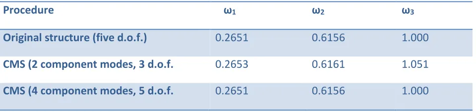
Results of analysis are summarized in table1

Table 1: Natural Frequencies of the structure shown in fig.1

Procedure ω1 ω2 ω3

Original structure (five d.o.f.) 0.2651 0.6156 1.000

CMS (2 component modes, 3 d.o.f. 0.2653 0.6161 1.051

CMS (4 component modes, 5 d.o.f. 0.2651 0.6156 1.000

V. CONCLUDING REMARKS

In this paper, the application of component mode synthesis method was studied with its prominent features and a numerical example is solved to get natural frequencies and mode shapes which give us the needed data concerning what excitation frequencies should be avoided. As expected, the reduced model yields the higher frequencies than the original model. Of course , there is no practical reason for retaining all modes, because the reduced problem is then of same size as the original, but it is reassuring that in this case component mode synthesis incurs no loss of accuracy.

REFERENCES:

1. Guyan R. J.,“ Reduction of Stiffness and Mass Matrices”, AIAA Journal, Vol. 3, No.2, February, 1965.

2. IronsB.,“Structural Eigenvalue Problems: Elination of unwanted Variables”, AIAA Journal, Vol. 3, No.5, pp 961-962, 1965.

3. Kidder R.L.,“Reduction of Structural Frequency Equations”, AIAA Journal, Vol. 11, No.6, p 892, 1973.

4. Shah V.N., Raymund M., “Analytical Selection of Masters for the Reduced Eigenvalue Problem” IJNME, Vol.18, No.1 pp89-98, 1982,

5. Ong J.H. , “Improved Automatic Masters for Eigenvalue Economization”, Finite Elements Analysis and Design , Vol 3, No. 2 , pp149-160, 1987,

6. Kim K. O. and Kang M.K., “Convergence Acceleration of Iterative Modal Reduction Methods”, AIAA Journal, Vol. 39, No.1, pp 134-140, 2001.

(10)

8. Craig R. R. Jr., “A review of Time-Domain and Frequency Domain Component Mode Synthesis Methods”, International Journal of Analytical and Modal Analysis, Vol.2, pp 57-72, 1987.

9. Hitchings D,“A Finite Element Dynamics Primer”, NAFEMS, Glasgow. U.K., 1992,

10. Noor A. K., Recent Advances and Applications of Reduction Methods, ASME ,Applied Mechanics Reviews, Vol.47, No.5, pp 125-146, 1994.

11. Shyu W.H., Ma Z.-D and Hulbert G.M. “A New Component Mode Synthesis Method : Quasi static Mode Compensation”, Finite Elements in Analysis and Design,Vol.24, No.4, pp 271-281, 1997.