Study on According to Modeling and Stability
of Single-Inverted-Pendulum Fuzzy Control
System Based on Petri net
Yuefeng Fang
1, Ran Jin
1,2,
Lingze Hu
31,2,3
School of Electronics and Computer, Zhejiang Wanli University, Ningbo, China) 2
School of Computer Science and Technology, Zhejiang University, Hangzhou, China)
ABSTRACT
This paper introduces the basics of fuzzy control and Petri nets. The Petri net models of the fuzzy control systems of balancing an inverted pendulum have been built. The simulation analysis is given to verify Petri net Modeling and stability theory of fuzzy control systems, and the simulation results demonstrate the validity of modeling methods and stability theorem presented in this paper.
Keywords: Single-Inverted-Pendulum; Fuzzy Control; Petri Net Modeling; Stability
I.INTRODUCTION
Stability is one of the most important indexes in control system. Petri net describe not only the variation of control process, but also the transference of data. It can be used to analyse the stability of the single-inverted-pendulum fuzzy control system. We can use Petri net as a modeling tool to make the Petri net model of the single-inverted-pendulum fuzzy control system. It shows the stability theory of the system, and does test and simulation as well[1][2][3]. [4]presents two new approaches for linguistic modeling which are suitable for stability analysis of linguistic models.[5]issue a hybrid system, which is integrated with the fuzzy system and Petri net models. We exploit the characteristics, imprecise or ambiguous information, of fuzzy theory to map the algorithm of crisp inputs and outputs, furthermore, model problems, product a nonlinear function, and final predict the next state transition of Petri net graphs. Tanaka[6]presents a sum of squares (SOS) approach to stability analysis of polynomial fuzzy systems. Our SOS approach provides two innovative and extensive results for the existing LMI approaches to Takagi-Sugeno fuzzy systems. [7] is concerned with the problem of quadratic stability analysis of nonlinear continuous-time control systems given by Takagi-Sugeno (T-S) fuzzy models. A new quadratic stability condition for the class of fuzzy control systems is presented in terms of solvability of linear matrix inequalities (LMIs).
II. PETRI NET Basic Concept
Petri net is a graphical modeling tool. It can describe the sequent, subsequent or synchronous relationship among the systems accurately, and the complex dynamic process of the system. Moreover, the Petri net model can be tested and verified by mathematical methods and tools.
Petri net is a kind of reticular information flow model, which can be classified as event and condition joints. Token Distribution which describes the state information is added based on the directed bipartite graphs of event and condition joints. The event - driven state evolves according to the initiating rules to reflect dynamic running process of the system. Normally, small rectangular is used to represent the event joints,i.e. transition joints, and small circular is to represent the condition joints, i.e. place joints. Directed arc can not appear among the transition joints or the place joints, but appears between the two. This kind of directed bipartite graphs are called nets. Some place joints of the nets are marked with Token to constitute the Petri net.
The following four structures are used to represent the Petri net graph:
Place, which is represented as a small circular O, i.e. P Element, is an area in which certain resources are placed. place is a information carrier always related to state concept. transition, which is represented as a small rectangular , i.e. T Element, is used to describe the transitions of resource consumption and the use and production of state elements. It describes the transition of the conditions involved in events, i.e. the new information derives from the existing information.
Directed Arc, which is represented as an arrow →, is used to connect place and transition. We cannot connect places or transitions directly. The arrow describes the causalities among places and among transitions. A transition can include many Input places and Out places. They are connected by Directed Arc.
Token, which is represented as a black dot, is an identification symbol. Token is also called Tokens in the place. Their variations in the place show the different state of the system. If a condition is represented in a place, it may include a Token or it may not. If the Token is included in the place, the condition is true, otherwise, the condition is false. If a place identifies a state, the state is fixed by the numbers of the Token in the place.
Definition of the Petri net
Definition 1. place/transition net, abbr. P/T net, is a 4-tuple. It can be described as N= (P, T, F, W). P is the place set.
T is the transition set.
p and T are nonempty finite and disjoint sets. Here, PT , PT .
F PT YP
is the Directed Arc set. W is the weight of the arc in F.
Definition 2. Petri net can be divided as a 5-tuple, i.e. P, T, I O,Mo.
1, 2 , n
P P P P
is the place set.
1, 2 , m
T T T T
is the transition set.
F PT YP
is the Directed Arc set. :
I PT Z is an input function. It identifies the set of the weight or the number of repetitions of Directed
Arc from P to T. And Z 0 , 1, is the set of nonnegative integers. :
O PT Z is an output function It identifies the set of the weight or the number of repetitions of
Directed Arc from T to P.
0
M
is an initial marking, i.e. the initial distributions of Token in each place.
Definition 3. Let P T I O, , , be Petri net structure. T is to identify the set of all input places of t. t
is to identify the number of all input places of t.
p
and p
are to represent the set of fore-and-aft conversions between input and output of P respectively.
The number of them are represented as p
and p
.
the procedures, for example, a machine is dealing with a component. transition describes the start and end of behaviors. The input and output functions of the arc places, transitions and Definitions from place to transition or from transition to place constitute the Petri net . The state of Petri net are presented by identifications, an identification is a vector, the length of which is the same as the number of place, i.e. the Kth element describes
the number of the Tokens in the Kth place. The initial marking of Petri net is M0. Token flows along the input and output arc among the places. The flows of the Token are determined by the activation of transition, so as to imitate the dynamic behavior of the system. The state of transition is changed with the activation of it, represented by identification. The activation of transition leads that Token flows among each place to imitate the dynamic behavior of the system. Thus the dynamic characteristics of the system is reflected.
Running Rules of Petri net
A dynamic behavior of the Petri net model is determined by its running rules. The Petri net runs according to the number and distribution of Token in the net. Tokens in place control the running of transitions. If each input place, which connects to the transition and whose arc is from the place to the transition, of the transition has at least one Token, the transition can be activated. Under this condition, the transition is called enability. The enability of an active table transition leads that each input place omits a Token, and each output place, which connects to the transition and whose arc is from the place to the transition, produces a Token. If the arc weight used is over 1, the number of Token in the input place of the transition should be at least equal to that of the arc weight. Then, the transition of the enability produces a corresponding number of Tokens in each output place according to the arc weight connected. The transition is actually an atomic operation. To remove the old Tokens from each input place and reinstall the new-produced Tokens in the output place is a indivisible complete operation.
The marking M of P N P T I O M, , , , 0 in Petri net is a function from set P to the non-negative integer set Z. M is an n-vector, in which, n p . The marking shows the number of Tokens in each place pi in Petri net.
The number and the distribution of Token change with the movement of Petri net. Petri net operates its system by firing the transition. And the marking is changed constantly. Burning in oxygen, iron wire can produce a black magnetic material, which can be uses as the raw materials of audio tapes and telecommunication apparatus,
and consists largely of F e O3 4. The chemical reaction equation that produces F e O3 4 is 3F e2O2 F e O3 4. It can be shown by Petri net as the following Figure1 and Figure2. Figure1 shows that there are three Fes and two
2
O
s before the reaction. Figure2 shows the state of the system after the transition being activated. Three Fes and
two O2s form one F e O3 4 .
Figure 1 Before the Transition Being Activated Figure 2 After the Transition Being Activated Definition 4. To the given marking M of Petri net. If the number of Token in each input place of the transition t is no less than the weight of the input arc, i.e.
t T, Pi t M, P W P ti ,
(1) then, transition t is enabled.
Definition 5. When a enabled transition t of marking M is activated, a new Marking M' is produced.
' ( ) ( ) ( ) ( ) , ( ) ( ) ( ( )
M p W p t p t t M p W p t p t t p P M
M p W p t W t p p t t M p o th e r
, , , , ) (2)
Definition 6. To the initial state M0 of system, if several transitions exist, then different transitions occur. and the reachable markings of M0 are different. The set of all reachable markings of M0 is called reachable set, marked as R N ,M0.
Definition 7. To the Petri net initial marked as M0, reachable graph describes all the reachable markings of Petri net. The reachable graph is a directed graph V,E. Here,V R N ,M0is a nodes set of directed graph, and E is a set of directed arc.
Those definitions are the common ones of Petri, based on which the Petri net is described in this paper. Besides those, there are some more complex Petri net, such as activated threshold one.
Basic Properties of Petri net
Petri net is a mathematical tool with many properties, which can generally be classified into two groups, i.e. behavioral and structural properties. The former are the properties related to initial markings of Petri net. Otherwise, those who are based on the initial markings are called structural properties, they are related to the topological structure of system only. Here we only consider those that are closely related to behavioral properties. After foundation of the model, we can make sure if the system contains some certain functional characteristics according to those properties.
Definition 8. In the P N P T I O M, , , , 0 of Petri net, if a transition sequence exists, M0 can be transferred into M by activation of the sequence, i.e.
M R N, M0 (3) M can be called reachable M0.
Reachable property is the reachable appointed running state of the system, which decides if a given marking M
belongs to R N ,M0 of Petri net. The reachable property is proved to be decidable, but usually exponent-complexed. Reachable property is the basis to analyse any dynamic characteristic of Petri net. An activation of enabled transition can change the marking, i.e. an activated sequence makes a marking sequence.
Definition 9. To a transition tT and all M R N ,M0 , if a transition sequence exists, the activation of which makes the transition enabled, then the transition is called Live. If all the transitions in Petri net are live, then the Petri net is live. The liveness of Petri net is related to that whether its disperse event dynamic system has deadlock. If the Petri net is live, then there is no deadlock when the system runs. Otherwise, the deadlock exists. Dead-transition and deadlock show the liveness of Petri net in a negative manner. If the
0
M R N,M
exists and the transition sequence does not exist, the activation of the sequence will enable t,
then the transition is dead transition. If the M R N ,M0 exists and no transition enability exists under M, then the Petri net includes a deadlock, the marking is a dead marking.
Definition 10. In P N P T I O M, , , , 0 of Petri net, if M R N ,M0 and k〉, (0 M pi) k, are
satisfied, then the place is called Pi p, and it is k bounded under initial M0. If Pi p is bounded, then the
Petri net is bounded. If K=1, then Pi p is safe. If Pi p is safe, then the Petri net is safe.
The security of Petri net is a special condition of boundedness.
Security ensures that the number of tokens in the place be only less than or equal to 1. If a certain place in the Petri net means a certain operation in the system, and the place is safe, then another operation cannot occur at the same time. For example, a place means a machine tool which can only make one work piece at the same time, then the place is safe. The security makes sure that no other work piece can be made before the present one is made.
Definition 11. In P N P T I O M, , , , 0 of Petri net, ifM R N ,M0and M0R N ,M0 are satisfied, then the Petri net with initial state is invertible. Reversibility ensures the system return to the initial state from any state, including failed state.
Definition 12. In Petri net, the matrix C:PT Z whose order set is PT is the incidence matrix, matrix
element is
i i i i i i
C p,t W( , )t s W s,t
(4)
In this function, i1 2,, ,n,j =1 2,, , m,m,z is a set of integers. The incidence matrix C which has n places and m transition is annm set of integers. Each row of matrix C corresponds to the transition, and each
column corresponds to the place.
Definition 13. In Petri net, the column vector whose order set is transition T is U:T Z , The initial marking
of Petri net is M0. By transition sequence,we get M R N ,M0 and 0
M M C U
(5)
Function 5 is the state equation of Petri net.
The Structures and Characteristics of Petri Net Model
1. The Structures of Petri Net Model
The common basic structure of Petri net model includes sequential structure, concurrency structure, conflict structure, synchronizing structure, merged structure and composite structure, and so on.
a. Sequential Structure b. Concurrency Structur c. Conflict Structure d. Synchronizing Structur e. Merged Structure f. Composite Structure
Figure3. Basic Structures of Petri Net
In sequential structure, transition t2 should be activated after transition t1, shown as 3a.
In concurrency structure, the activation of anyone of the transition t1, t2 and t3 enable the other two be activated, shown as 3b.
In synchronizing structure, only when the resources are all equipped, can the transition be activated, shown as 3d.
In merged structure, the activations of transition t1, t2 and t3 affect the same resource, shown as 3e. In composite structure, it is a state includes both concurrency and conflict, shown as 3f.
2 The Characteristics of Petri Net Model
Petri net can present the system structure well. It describes the concurrent, conflicting, synchronizing and
sequential relations in system. The composite models which are shown as graphs are more intuitive, understandable and practical. For describing the conflict and concurrency, it is extremely excellent. Meanwhile,
as a mathematical object which is strictly defined, the Petri net has a solid theoretical foundation in Mathematics. the modeling capability of Petri net is proved to be equal to the Turning Machine.
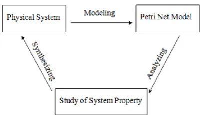
Figure 4 Modeling and Analyzing of Petri Net System
Petri net is a modeling tool of the system, it is used to design and analyze the system. It focuses on the variations
and their conditions, influences and relations. The modeling and analyzing processes of Petri net are shown as Figure4.
The system model of Petri has the following characteristics.
A. It simulates system according to organization structure, control and management, and excludes the physical
and chemical principles that the system relays on.
B. It describes the dependency and independency among the events in the system accurately, which exist
objectively among the events, and are independent of the way we observe. C. It applies to describe the system characterized by the rules of behaviors. D. It describes the structure and the behaviour of system a unified language.
E. The network system is an independent research object, and possesses the dynamical behaviors which have nothing to do with the application environments.
F. In different field, network system has different functions, so as to bridge various fields. G. Network system applies to describe the synchronizing concurrent systems.
The Analytical Methods of Petri Net
After being built up according to the physical meaning of the system, the Petri net model can analyze the net with its theory. General speaking, the analytical methods include the followings.
A. Reachable Tree
It is the most intuitive method, which represents all the state reachable in a tree view. The reachable tree method describes the state that the system can reach under the initial state, and produces a given network system.
series of transitions. And each new marking can then produce more new markings by different transitions. By that analogy, such a process can produce a marking tree. And then a tree diagram, which is called reachable tree,
is formed with the root of initial marking M0. With those reachable trees, the marking start from the initial one can be described as joints, and each arch represents the activation of the enabled transition. It ensure that the
network transit from one marking into another. The reachable tree describes the dynamical behavioral characteristics of the system. To a bounded Petri net, it can represent the system behaviors actually, and corresponds to the finite state. While, to boundless Petri net, it can only partly reflect. The reachable tree method
can be used to present the security, boundness, conservativeness and coverability. It has some disadvantages either, it can neither solve reachable and activity problems nor judge the activation queue of the transitions. It is
for a certain initial marking, and a new initial marking means a new reachable tree is needed. When many concurrency conflict transitions occur in the system, state space explosion will happen. It has no regard for the concurrency issues, and cannot distinguish the concurrencies and conflicts in the transitions. Due to the
characteristic of explosivity, the reachable tree method is not suitable for the large scale system. The complexity of the reachable tree changes exponentially according to the scale of the system, so it is usually used in the small
scale network.
B. Incidence Matrix and State Equation
In engineering, the dynamical behaviorus characteristics can usually be described by the difference equation and
differential equation. Similarly in Petri net, behavior characteristics of the system can be described by incidence matrices and state equations. The application of state transition equation can avoid occurring reachable state in
the system. By relevant knowledge of linear algebra, it presents some characteristics of the Petri net briefly, especially the structural characteristics. But this method cannot well present the dynamic characteristics of the system. Generally speaking, it is only a necessary condition but not a sufficient condition to describe the
reachable characteristics. It is sufficient only to describe the conflict-free subclass. Moreover, while modeling the system, the Petri net has its inherent uncertainty and the solution of the state equation should be nonnegative,
so state equation should apply only to partial subclasses of the network.
To Petri net which is not a pure network, if the place is the input and output place of the same transition, the
offset will occur in the incidence matrices, which can not present the real structure of the Petri net then. So these non-pure-networks should be changed or reduced into pure networks to be identified by the incidence matrices.
C. Analysis and Reduction Technique
Analysis and reduction technique simplifies the system by certain rules, with the original characteristics unchanged. It is used to analyze some large-scale net systems. It can reduce the scale of the net systems while
retaining partial behavioral characteristics, such as activity, security and boundness. Reduction is a homomorphic transformation process. It reduces a complex Petri net into a simple one with some of the characteristics unchanged. It reduces the space of the reachable state and provides various information to grasp
the characteristics of the initial network by analyzing the simple one.
D. Linguistic Method of Petri Net
the sequence of events can be controlled to schedule the resources reasonably and effectively. Petri net can be regarded as a kind of automaton, the languages produced by which can be use to define their calculating and modeling abilities. And the system behaviors can be analyzed by the sequences raised. This method applies to
theoretical qualitative study, but has poor operation in practice.
III. MODELING AND SIMULATION ANALYSIS OF SINGLE-INVERTED-PENDULUM FUZZY CONTROL SYSTEM PETRI NET
A. Single-Inverted-Pendulum Fuzzy Control System
In this paper, we describe how to use Petri net to model the fuzzy control system by the traditional questions of
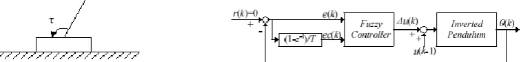
balancing inverted pendulum. Shown as Figure 5, is the clockwise flip angle from the pendulum rod to the vertical direction, marked by Radian, and the clockwise direction is positive. is the torque pressing counterclockwise on the rod, marked by Newton Meter, and counterclockwise direction is positive, and u(t) is the controlled variable. The differential equation of the system is the following.
2 2
2
( )
lg s in ( ) ( )
d t
m l m t u t d t
(6)
In function 6, m is the weight of the rod, marked by newton, l is the length of the rod, marked by meter, t is the time, marked by second. Our aim is to balance the inverted pendulum.
Figure 5. Single-Inverted-Pendulum System Figure 6.Single-Inverted-Pendulum Fuzzy Control System
In order to control the inverted pendulum, we can set up a digital fuzzy control system, shown as Figure 6. And r(k) is the anticipating angle of the rod at sampling time k. The initial angle between inverted pendulum and the
vertical direction is nonzero, i.e. ( 0 ) 0. Our aim is to balance the inverted pendulum, and make the rod
vertical, i.e. k, r k( ) 0. The inputs of the fuzzy controller are e(k) and ec(k). Here e(k) is the error between
r(k) and ( )k , and ec(k) is the variation of the error. The output of the fuzzy controller is △u(k). It is the increment of the control input to single inverted pendulum.
B. Petri Net Model of Single-Inverted-Pendulum Fuzzy Control System
Most of the actual operations in the fuzzy control system adopt single fuzzy model. And the membership function of the set E is defined as the following.
1 x = e ( )
0
e x
o t h e r w i s e
(7)
A. The linguistic variables of the input e(k) and ec(k) in the fuzzy controller are set as E and EC respectively. The fuzzy subsets of E and EC are both {N, Z, P}, and the membership function of the fuzzy subset in the
B. The linguistic variables of the output △u(k) in the fuzzy controller is set as △U, with the universe of {-0.6,
-0.3, 0, 0.3,0.6 }. The fuzzy subsets of △U is classified as {NB, N, Z, P, PB}, and each membership function of the fuzzy subset in the universe is presented as the following Figure8.
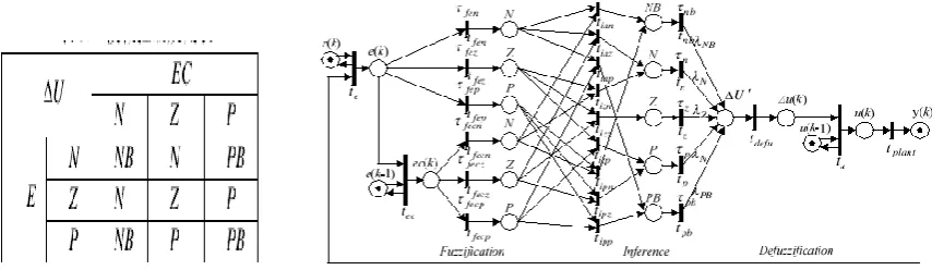
C. The fuzzy control rule database of the single-inverted-pendulum fuzzy control system is established as
Figure9. In the rule database, rule R1 is necessary, and here,
1:
R If E Z and EC=Z Then U Z
. That is to say, the moment presses on the rod keeps
constant when is in the vertical state.
Figure 7. input e(k) and ec(k) membership function Figure 8 Membership Function of Output △u(k)
Figure 9. Fuzzy Control Rule Table Figure 10. Petri Net Model of Single-Inverted-Pendulum Fuzzy Control System
The Petri net of single-inverted-pendulum fuzzy control system in Figure6 can be shown in the form of Figure10.
In the Petri net model of fuzzy control system shown as Figure10, to all k, the order of transition activation should satisfy the following transition sequence.
k t te e c tfe x tfe c y tip qt ts d e fut tu p la n t
( & )
(9)
In which,
fex fen fez fep fecy fecn fecz fecp s n b n z p p b ip q i n n in z in p izn izz izp ip n ip z ip p t t t t ,t t t t ,t t t t t t ,t t t t t t t t t t ,
& is the AND operation, and is the OR operation.
Modeling has the following transition-activating sequences.
e k r k k
( ) ( ) ( ).
Step 2. When the input place has tokens and transition te c has been activated, ec(k) can be gotten by
calculating e c k( ) ( ) ( e k e k 1).
Step 3. Deviation e(k) is fuzzed into the fuzzy language variable E, the membership function based on deviation
e(k) depends on the the transitions activated in the tfe ntfe z tfe p
. If the place e(k) has tokens whose value is over
the threshold value f e n,f e z,f e p of those transitions, then the corresponding transitions can be activated.
After activation, the the value of the token in the output place represents the membership of the each linguistic value corresponding. In the same way, deviation ec(k) is fuzzed into the fuzzy language variable EC, the
membership function based on ec(k) depends on the the transitions activated in the tfe c ntfe c z tfe c p
. If the place ec(k)
has tokens whose value satisfies the threshold value f e c n,f e c,zf e c p of those transitions, then the
corresponding transitions can be activated.
Step 4. Based on the fuzzy-control rule shown as Table 1, the fuzzy inference can be realized by the inference synthesis algorithm. First, the conclusion of each rule can be gotten according to the rule table. Its value can be linguistic value of fuzzy output control quantity , which are NB N, Z, P, B. It depends on the transitions
activated in the fuzzy control rule in n in z in p iz n iz z iz p ip n ip z ip p
t t t t t t t t t
. Only if the output place has tokens, and
the membership function of output △u(k) satisfies the threshold value tn b,tn,tn,tp,tp b
, can the transition
n b n z p p b
t t t t t
be activated. The weight after activation is N B N P P B 1, the corresponding fuzzy
conclusion of each rule can be defined. The fuzzy inference can be realized by the fuzzy set output according to inference synthesis.
Step 5. If the output fuzzy set has tokens and transition td e f u is activated, the fuzzy result can be changed in to
exact value △u(k).
Step 6. If the input place u(k)has tokens and the transition is activated, the control input u(k) of the inverted pendulum can be calculated by ( ) (u k u k1) u k( ).
Step 7. If place u(k) has tokens and transition tp l a n t is activated, the angle ( )k that deviate from rod to the
vertical position can be measured.
Then starting from Step 1, a new cycle recommences. So on, the whole Petri net runs under this transition activation sequence.
Next, we will analyze the stability of the system by the Petri net model built.
C. Simulation Analysis on Stability of Single-Inverted-Pendulum Fuzzy Control System Petri Net
The Petri net model of single-inverted-pendulum fuzzy control system is shown as Figure9. Let the state
variable be x1 and x2 d /d t, in which x1 is the angular value of Figure5, marked by radian, x2 is the angular speed, marked by radians/second. We can know the followings.
2 1
2 2 ( / ) s in 1 (1 / )
x x
x g l x m l u
(10)
If x1 is very small, we get
s inx1 x1 (11)
2 1
2 2 ( / ) 1 (1 / )
x x
x g l x m l u
(12)
In Equation 12, x1 is marked by radian and x2 is marked by radians/second. Let l g and 2
1 8 0 / ( )
m g
, the linear discrete state space of Equation 12 can be described by the following differential equations, in which k is the sampling interval.
1 1 2
2 1 2
( 1) ( ) ( )
( 1) ( ) ( ) ( )
( 1) ( ) ( 1)
x k x k x k x k x k x k u k u k u k u k
(13)
The fuzzy controller is designed with the input x1 and x2, By fuzzing the membership function shown in Figure 7, the inference machine produces inferences based on the fuzzy control rule database shown as Table. 1.
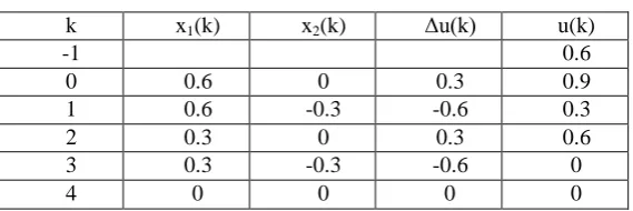
Combining the defuzzification of Fig. 8 and the result of Equation 13, we can get the simulation result shown as Table 1
Table 1. Simulation Result
k x1(k) x2(k) Δu(k) u(k)
-1 0.6
0 0.6 0 0.3 0.9
1 0.6 -0.3 -0.6 0.3
2 0.3 0 0.3 0.6
3 0.3 -0.3 -0.6 0
4 0 0 0 0
In this table, u( 1) , which is meaningless, can be gotten by Equation 10. x1( 0 )0 .6 and x2( 0 ) 0 are the initial state that the rod deviates from the vertical position. By Table 2, we know that a nonnegative integer 3
exists. When k>3, the simulation result of x1( )k x2( )k 0 shows that the fuzzy control system shown by Figure 6 is stable. And when k>3, it always exists that Z C Z. And the activation sequence of transition
Z C Z is always k t te e c(tfe x&tfe c y)tiz zt tz d e fut tu p la n t
. It verifies the stability theorem of the fuzzy control system.
CONCLUSIONS
Taking for example the control of the single-inverted-pendulum control, and employing the modeling method proposed, we establish the Petri net model according to the fuzzy control system, and do a detailed analysis of which. We also use Matlab to do the simulation, by analyzing which the modeling method and the stability theorem are verified. The simulation result shows that the modeling method and the stability theorem are effective.
This paper focuses on the control of the single-inverted-pendulum control, to discuss the modeling method and the stability of fuzzy control system based on Petri net. There are still some problems need to be studied further.
A. The stability theorem of fuzzy control system is mainly put forward by analyzing the system stability based on simulation. While in actual system analysis, how to judge and analyze the stability of fuzzy control system more intuitively needs a further study. Those such as the stability criterion of traditional control should be given.
B. In this paper, the stability of system is judged by the activation sequences of the transition. The activation sequences of the transition are actually more than those given ones. Moreover, those sequences are activated circularly. In this case, the system can still be judged as stable. a further study is needed to improve the theorem.
research on other characteristics of the fuzzy control system is needed to be solved in further research.
ACKNOWLEDGMENT
This Work is Supported by Public welfare technology research project of Zhejiang Province, under grant by no. 2013C31080, and by the Ningbo Natural Science Foundation under grant No.2015A610141, and by the Zhejiang Postdoctoral Project, and by the National Undergraduate Training Programs for Innovation and Entrepreneurship under grant No. 201610876004, and by the the new-shoot Talents Program of Zhejiang Province under grant No. 2016R420021.
REFERENCES
[1]. Zhi-Hong Xiu and Guang Ren. Stability analysis and systematic design of Takagi-Sugeno fuzzy control systems. Fuzzy Sets and Systems. April 2005, 151(1).119-138
[2]. Gui-Chen Zhang, Song-Tao Zhang, Guang Ren. A Piecewise Fuzzy Lyapunov Function Approach to Stability Analysis of Discrete T-S Fuzzy System. Proceedings of the 4th International Conference on Fuzzy Systems and Knowledge Discovery. August 2007, 1。316-320
[3]. Xiaojun Ban, X.Z. Gao, Xianlin Huang and A.V. Vasilakos. Stability analysis of the simplest Takagi-Sugeno fuzzy control system using circle criterion, Information Sciences. August 2007, 177(20). 4387-4409
[4]. A. A. Suratgar and S. K. Nikravesh. Stability Analysis of Variation Model for Linguistic Fuzzy Modeling. The 12th IEEE International Conference on Fuzzy Systems. May 2003, 1。108一113
[5]. Rong-Hou Wu, et.al. A Hybrid System with Petri Net and Fuzzy Theory. Proceedings of the 9th Joint Conference on Information Sciences. October 2006. 1269-1272
[6]. Kazuo Tanaka, Hiroto Yoshida, Hiroshi Ohtake and Hua O. Wang. A Sum of Squares Approach to Stability Analysis of Polynomial Fuzzy Systems. 2007 American Control Conference. July 2007. 4071-4076
[7]. Guang-Hong Yang and Jiuxiang Dong. Quadratic Stability Analysis of Fuzzy Control Systems. 2006 American Control Conference. June 2006. 4344-4349
[8]. Chih-Peng Huang andYau-Tarng Juang. A projection scheme to stability analysis of discrete T-S fuzzy models. Mathematics and Computers in Simulation. March 2004,64(6). 643-648
[9]. Wu, W.J., Yue, B.Z., Huang, H.: Coupling dynamic analy-sis of spacecraft with multiple cylindrical tanks and flexibleappendages. Acta Mech. Sin. 32, 144–155 (2015). doi:10.1007/s10409-015-0497-3
[10]. Miao, N., Wang, T.S., Li, J.F.: Research progress of liquid slosh-ing in microgravity. Mech. Eng. 38, 229-236 (2016). doi:10.6052/1000-0879-15-185
[11]. Farid, M., Gendelman, O.V.: Internal resonances and dynamicresponses in equivalent mechanical model of partially liquid-filledvessel. J. Sound. Vib. 379,191-212 (2016). doi:10.1016/j.jsv.2016.05.046