INTERFACIAL HEAT TRANSFER COEFFICIENT ESTIMATION
DURING SOLIDIFICATION OF RECTANGULAR ALUMINUM ALLOY
CASTING USING TWO DIFFERENT INVERSE METHODS
R. Rajaraman
a, L. Anna Gowsalya
b*and R. Velraj
ca Professor, Department of Mechanical Engineering, School of Mechanical Sciences, SRM Institute of Science and Technology, Vadapalani Campus,
Chennai, Tamilnadu, India- 600 026. Email: [email protected]
b Assistant Professor, Department of Mechanical Engineering, School of Mechanical Sciences, B.S. Abdur Rahman Crescent Institute of Science and
Technology, Vandalur, Chennai, Tamilnadu, India- 600 048, E-mail: [email protected]
c Professor and Director, Institute for Energy Studies, College of Engineering Guindy, Anna University, Chennai, Tamilnadu, India- 600 025,
Email: [email protected]
A
BSTRACTTo get accurate results in casting simulations, prediction of interfacial heat transfer coefficient (IHTC) is imperative. In this paper an attempt has been made for estimating IHTC during solidification process of a rectangular aluminium alloy casting in a sand mould. The cast temperature and mould temperature are measured during the experimental process at different time intervals during the process of solidification. Two different inverse methods, namely control volume and Beck’s approach are used to estimate the heat flux and temperature at the mould surface by using the experimentally measured temperatures. In the case of control volume technique, the partial derivative of one dimensional transient heat conduction equation for the rectangular geometry is modified into an ordinary differential derivative with respect to time. These equations are solved sequentially to get the heat flux and temperature at the mould surface. The same partial derivatives are solved using the function specification method in Beck’s approach. The IHTC values obtained by these two approaches are in good agreement with the results cited in literature.
Keywords: Control volume, inverse heat conduction, interfacial heat transfer coefficient, rectangular geometry, solidification.
1. INTRODUCTION
The microstructure and the absence of defects influence the quality of casting metals and alloys during solidification. This in turn depends on the process of solidification. Increased competitiveness in the casting industry requires reduced scrap and lower design cycle time. To meet this requirement, computer simulation to the casting solidification is considered as an appropriate tool.
The input parameters mainly influence the accuracy of the casting simulation results. The heat transfer coefficient, particularly at the casting–mould interface is one of the key input parameters, which plays a key role in the precise modeling of the solidification process. An air gap is formed between the solidifying metal and the mould inner wall due to the shrinkage of molten metal and the release of metal oxide gases during solidification. This air gap acts as a thermal barrier for the heat flow and hence influences the cooling rate. This resistance causes considerable difference in the temperature of the mould surface compared with the cast surface.
The drop in temperature from the surface of the cast to the surface of the mould as well as heat transfer is represented by a parameter called interfacial heat transfer coefficient ‘h’ (IHTC). The ‘h (IHTC)’ determines the heat flow from the metal to the mould at any time and is represented by equation (1).
𝑞(𝑡)= ℎ(𝑡)[𝑇𝑐(𝑡)− 𝑇𝑚𝑠(𝑡)] (1)
*Corresponding author:Email:[email protected]
The following two approaches are generally used to determine the IHTC, at the metal-mould interface during casting process.
1. Air gap measurement technique 2. Inverse method
In air gap measurement technique, the size of the gap measured by a linear transducer is used to estimate the IHTC (Ho and Pehlke, 1984, 1985). Many factors such as molten metal temperature, its flow properties, properties of mould materials, riser height etc. are found as the influencing parameters for the IHTC. The increased riser pressure was found to be another parameter that accelerates the heat transfer due to increased contact of metal-mould after pouring (Lukens et al., 1990). In the second approach, the temperatures at certain locations of the metal and the mould are measured experimentally and the value of IHTC is estimated by the application of inverse method. The IHTC is calculated based on the measured cast temperature, the estimated mould surface temperature, and the estimated mould surface heat flux. It is very difficult to calculate the surface heat flux and surface temperature of the mould and this leads to the inverse heat conduction problem (IHCP) or Ill-posed problem. The Ill-posed nature of the IHCP makes it more difficult to solve than the direct heat conduction problems (DHCP).
The ill posed problems (IHCP) are solved by a variety of solution techniques (Burggraf, 1964; Beck, 1970 & 1985; Hsu et al., 1992; Masanori, 2000). Taler and Zima (Taler and Zima, 1999) developed control volume technique as one of the solution procedures for multidimensional IHCP. The authors assumed same thermal conductivity
Frontiers in Heat and Mass Transfer
for both the metal and the mould, which was one of the insights of a source for deviation.
The determination of IHTC by the inverse method can be accomplished by two different approaches. The first approach is based on the specification of an objective function and it maximizes or minimizes the function in order to get the exact value of surface heat flux or surface temperature at the mould. This method is known as Beck’s function specification method. The other approach is based on energy balance applied to different control volumes for the estimation of the heat flux and temperature at the surface of the mould. This approach is known as control volume approach.
Many researchers considered various geometries, materials and solution techniques for the estimation of IHTC. Lau (Lau et al., 1998) characterized the variation of the IHTC with time into three stages. Kuo ( Kuo et al., 2001) measured the IHTC at the interface between aluminum alloy casting and metallic mould with various coatings. They studied the effects with two types of metallic mould and different coating materials with three coating thicknesses. The molten metal melt superheats have a significant role on the peak heat flux in the initial stages of solidification (Narayan Prabhu and Ravishankar, 2003). Narayan Prabhu and Suresha (Narayan Prabhu and Suresha, 2004) investigated the heat transfer during solidification of an Al-Cu-Si alloy and commercial pure Ti in single steel, graphite, and graphite-lined metallic moulds. The experiments showed that increased melt superheats and higher thermal conductivity of the mould material led to an increase in the peak heat flux at the metal-mould interface.
Basil and Stavros (Basil and Stavros, 2007) developed a unique and versatile approach to measure the IHTC and observed that the higher temperature of liquid metal produced higher values of IHTC. The surface roughness of the mould impacts inversely on the value of IHTC and the formation of the air gap. The authors established a correlation between the IHTC and air gap size.
The thickness of the cast section has significant effect on IHTC. Woodbury (Woodbury et al., 2000) determined the IHTC by direct coefficient approach during resin-bonded sand casting of aluminum (A356) for three different section thicknesses. Narayan Prabhu (Narayan Prabhu et al., 2005) studied the heat flow at the casting-mould interface during the solidification of Al-Cu-Si alloy (LM 21) plates on thick and thin moulds. The interfacial heat flux transients estimated by inverse approach had higher values for thin moulds, although the solidification time was lower.
A few research papers are available for the comparison of the value of IHTC obtained by the air gap and the inverse approach. In a comparative study of these two approaches of estimating IHTC, Hwang (Hwang et al., 1994) observed the IHTC estimated by the air gap method to be around 10 times smaller than the IHTC value obtained by the inverse approach. The estimation of IHTC for the air gap method is basically assumed conduction heat transfer in the gap between metal and mould. This assumption gives deviated results of IHTC, since the heat transfer by other modes are also possible in the gap. The unevenness of the surface and the irregularities present may render the method ineffective.
Ramesh (Ramesh et al., 2009) carried out thermo mechanical simulation for Al-Si alloy using commercial code. They validated the simulated cooling curves for a cylindrical casting with the experimental data from the literature. Rajaraman and Velraj (Rajaraman R and Velraj R, 2009) estimated and compared IHTC for a cylindrical aluminum alloy casting with sand mould using two different inverse methods, namely control volume (CV) technique and Beck’s algorithm approach. They reported that the control volume technique gave accurate and reliable results since this approach did not involve any complex iteration for the calculation of IHTC.
Lazar Kovacevic (Lazar Kovacevic et al., 2012) estimated IHTC by an iterative algorithm based on function specification method by using
thermal history obtained from the experiment and solving the inverse heat conduction problem (IHCP) for rectangular geometry. He described IHTC as a function of casting surface temperature and proposed a correlation to compare the estimated IHTC values. Zhang (Zhang et al., 2017) estimated the IHTC at the metal mould interface by applying non-linear estimation method during the solidification of low pressure sand casting for a plate shaped casting with different thickness for an aluminum alloy. They observed that the value of IHTC first increased to a maximum and then decreased and after that it remains constant.
Vaisleiou (Vaisleiou et al., 2017) developed a Genetic Algorithm (GA) approach to determine the value of heat transfer coefficient (HTC) between Al-Si cast and steel mould, considering two different geometries. The GA simulated the temperature by getting the different values of HTC as input and the simulation continued until there was a small difference between the simulated and the actual measured temperatures obtained.
The study of the literature has revealed that most of the researchers used the inverse method for the estimation of IHTC and their results differed significantly based on the geometry and boundary conditions adopted. However, the accuracies of the different inverse solution methodologies were not compared by many authors with the same boundary conditions. Only limited papers are available for the comparison of IHTCs estimated using different inverse methods. Hence in order to check the accuracies of the inverse methods, in the present work two different approaches (i) Beck’s approach and (ii) control volume approach have been applied for the rectangular geometry and the results obtained have been compared.
In this work, heat flux and temperature at the mould surface have been estimated by both the approaches for rectangular geometry castings. The calculation of IHTC requires the temperature values at cast and at some convenient locations marked inside the mould, which have been measured experimentally. The IHTC values have been estimated for the rectangular geometry casting by both the approaches using computer programs. The estimated IHTC values for the rectangular geometry casting by the control volume techniques have been compared with those values obtained by Beck’s approach.
2. INVERSE MODELING FOR RECTANGULAR
GEOMETRY CASTING
2.1 Inverse heat conduction problem
All Dimensions are in mm
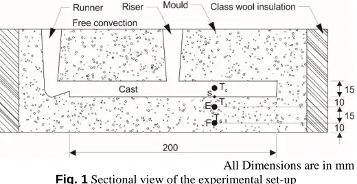
Fig. 1 Sectional view of the experimental set-up
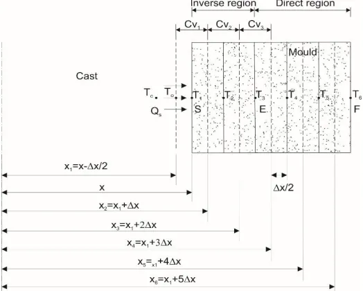
(calculated surface heat flux and temperature) at metal mould interface are not known at the location S which is calculated from the known (temperature measured) direct region. There are three control volumes being taken in the inverse region for the analysis and energy balance is applied over the individual control volume to obtain the unknown boundary condition (temperature at mould surface and heat flux at mould surface) at location ‘S’.
Fig. 2 1-D Inverse heat conduction problem showing control volume grid in the inverse region
The governing 1-D transient heat conduction equation for solidification process of a rectangular geometry is given in equation (2):
𝜕2𝑇
𝜕𝑥2=
1 𝛼
𝜕𝑇
𝜕𝑡 (2)
2.2 Initial conditions
1. The mould is maintained at constant temperature when t = 0 i.e., T(x,t) = Tini (Known value when t = 0)
2. A known small value of heat flux is applied at the mould interface when t = 0 and this small value of heat flux is corrected
i.e., q(x = x1 + , 0) = small assumed heat flux value
2.3 Boundary condition at direct region
1. The temperature at any time t is known at location E (Measured temperature)
i.e., T(x = x3 + , t) = T3
2. The temperature at any time t is known at location F (Measured temperature)
i.e., T(x = x6 + , t) = T6
Table 1 Properties of Aluminum alloy and Green sand
Material Density
kg/m3
Specific heat J/(kgK)
Thermal conductivity W/mK
Cast metal (Al 6061) 2650 1200 150
Green sand 1700 950 0.45
3. SOLIDIFICATION OF RECTANGULAR GEOMETRY
CASTING
3.1 Experimental set-up
The sectional view of experimental set-up for rectangular pattern along with cope and drag is shown in figure 1. A solid pattern of size 150 mm 200 mm x 15 mm was used for the preparation of the cast. To achieve one dimensional heat transfer, the four side walls of the mould were insulated using glass wool with wall of thickness 20 mm. The heat transfer was allowed only in a direction perpendicular to the longer face of the rectangular plate.
There were three K type chrome-alumel thermocouples used to measure the temperature at the cast and the mould. One thermocouple (Tc) was directly placed in the mould cavity to measure the cast temperature. The other two thermocouples were placed at location E (T3) and F (T6) in the mould at distances of 10 mm and 25 mm from the bottom of the mould surface respectively. To minimize the error due to the presence of riser, the thermocouples T3 and T6 were positioned on the opposite side of the riser. The positions of the thermocouples are shown in figure 1. A data acquisition system with 16-channel along with thermocouples was used to measure the temperature of the cast and mould for every 10 second intervals. The data acquisition system was interfaced with a computer to record the temperature data.
3.2 Experimental procedure
A 15 kW electric arc furnace was used for the melting of Aluminum alloy. A controller provided in the furnace was used to monitor the temperature of the alloy material. Once the set temperature reached in the furnace, the molten metal at 840oC, was poured into the rectangular cavity through the runner. During the pouring of the metal, it is always melted above its melting point to ensure the good fluidity of the molten alloy and for the filling. Since the mould wall was insulated, the heat transferred from the cast to the mould ensured one dimensional heat transfer. After pouring the temperatures were recorded and the high temperature molten metal cast was allowed to cool. This was continued till the difference in the temperature of the cast and mould was low. The temperatures at the cast and mould were recorded by the thermocouples placed using the 16 channel computer integrated data acquisition system for every 10 seconds. The temperature history measured experimentally with respect to time at the cast (Tc) and at the two locations E and F (T3 and T6) in the sand mould were plotted in figure 3.
Fig. 3 Variations of the cast temperature and sand mould temperature with respect to time during solidification
2 x
2 x
2 x
0
150 300 450 600 750 900
0 150 300 450 600 750 900
T
em
p
era
tu
re
(
ºC)
Time (s)
4. EVALUATION OF INTERFACIAL HEAT TRANSFER COEFFICIENT BY CONTROL VOLUME APPROACH
4.1 Control volume approach
The main principle of control volume approach is based on the application energy balance over different control volumes surrounded by the known grid points. In this method, the mould is divided into a number of grid points and each nodal point is surrounded by a control volume. At each nodal point, the energy balance is applied to determine the unknown mould surface temperature and surface heat flux. The control volumes used for the rectangular geometry casting is illustrated figure 2.
4.2 Energy balance for the rectangular casting
In this approach the measured temperatures at T3 and T4 were used as known values at discrete time intervals. The energy balance was first applied to the nodal point 3 or control volume 3 (CV3) partly in the inverse region and partly in the direct region as per figure 2. The unknown surface temperature (T2) in the inverse region was evaluated using the measured temperature (T3) and the calculated heat flux QE in the direct region at nodal point E. Further, the mould surface temperature at T1 location was found by applying energy balance at the control volume 2 (CV2). All the unknown temperatures were determined in terms of measured values at T3. The boundary conditions at the mould surface i.e., the heat flow (QS) and the temperature (T1) were determined by the energy balance applied over the control volume.
Eq. (3) gives the one dimensional heat conduction equation for a rectangular geometry at point E where the temperatures are measured with respect to time (known).
𝑄𝐸= 𝑘𝑚 𝐴 (𝑇3∆𝑥−𝑇4) = 𝑘𝑚 𝑏 𝑙(𝑇3∆𝑥−𝑇4) (3)
Re-arranging the Eq. (3), we obtain Eq. (4):
𝑇4= 𝑇3−𝑄𝑘𝐸 ∆𝑥
𝑚 𝑏𝑙 (4)
The heat flow QE was determined from the experimental temperatures T3 and T4 using Fourier’s law of heat conduction at any instant; this region was called direct region and it was treated as the direct heat conduction problem (DHCP). At nodal point E the measured temperature (T3) and the heat flux were known values for various time steps but the boundary conditions at point S (mould surface), were not known. The unknown values at S were calculated from the known point E. Utilizing the heat conduction equation at the mould surface S, Eq. (5) was obtained:
𝑄𝑠= 𝑘𝑐 𝐴 (𝑇0∆𝑥−𝑇1)= 𝑘𝑐 𝑏𝑙 (𝑇0∆𝑥−𝑇1) (5)
On re-arranging the Eq. (5), we get Eq. (6):
𝑇0= 𝑇1+ 𝑄𝑘𝑠∆𝑥
𝑐 𝑏𝑙 (6)
To start with control volume approach, the energy balance was made over the control volume 3, where the temperature was known from the experimentally measured data and Eq. (7) gives the energy balance:
(𝑥4− 𝑥3)𝜌𝑚𝑐𝑚𝑑𝑇𝑑𝑡3=𝑘𝑚(𝑇∆𝑥2−𝑇3)− 𝑘𝑚(𝑇∆𝑥3−𝑇4) (7)
From Eq. (4) substituting T4 and rearranging, Eq. (8) is arrived:
𝑇2= 𝑇3+∆𝑥
2
𝛼𝑚
𝑑𝑇3
𝑑𝑡+ 𝑄𝐸∆𝑥
𝑘𝑚 𝑏𝑙 (8)
Eq. (9) is obtained by applying energy balance equation from the control volume 2:
(𝑥3− 𝑥2)𝜌𝑚𝑐𝑚𝑑𝑇𝑑𝑡2=𝑘𝑚(𝑇∆𝑥1−𝑇2)− 𝑘𝑚(𝑇∆𝑥2−𝑇3) (9)
On substitution of T2 and in Eq. (9) and on rearrangement, Eq. (10)
is obtained:
𝑇1= 𝑇3+3 ∆𝑥
2
𝛼𝑚
𝑑𝑇3
𝑑𝑡 + ∆𝑥4
𝛼𝑚2
𝑑2𝑇 3
𝑑𝑡2 +
2 𝑄𝐸∆𝑥
𝑘𝑚 𝑏𝑙 +
∆𝑥3
𝑘𝑚𝛼𝑚 𝑏𝑙
𝑑𝑄𝐸
𝑑𝑡
(10)
By applying energy balance at control volume 1, Eq. (11) is obtained:
{[𝑥2− (𝑥2−∆𝑥2)] 𝜌𝑚𝑐𝑚+ [(𝑥2−∆𝑥2) − 𝑥1] 𝜌𝑐𝑐𝑐 }𝑑𝑇𝑑𝑡1= 𝑘𝑐(𝑇∆𝑥0−𝑇1)− 𝑘𝑚(𝑇1−𝑇2)
∆𝑥 (11)
After rearrangement, Eq. (11) can be written as
(𝜌𝑚𝑐𝑚+ 𝜌𝑐𝑐𝑐)∆𝑥
2
2 𝑑𝑇1
𝑑𝑡 = 𝑘𝑐(𝑇0− 𝑇1) − 𝑘𝑚(𝑇0− 𝑇1) (12)
On substitution of T0, T1, T2 and in Eq. (12) and on rearrangement,
Eq. (13) is obtained:
𝑄𝑠= 𝑄𝐸+∆𝑥2 𝑏𝑙 (5 𝜌𝑚𝑐𝑚+ 𝜌𝑐 𝑐𝑐)𝑑𝑇𝑑𝑡3+ ∆𝑥
3
2𝛼𝑚 𝑏𝑙 (5 𝜌𝑚𝑐𝑚+ 3𝜌𝑐𝑐𝑐)𝑑
2𝑇3
𝑑𝑡2 +
∆𝑥5
2𝛼𝑚2 𝑏𝑙 (𝜌𝑚𝑐𝑚+ 𝜌𝑐𝑐𝑐)
𝑑3𝑇3
𝑑𝑡3 +
∆𝑥2
𝑘𝑚((2 𝜌𝑚𝑐𝑚+ 𝜌𝑐 𝑐𝑐)𝑑𝑄𝑑𝑡𝐸+ ∆𝑥
4
2 𝑘𝑚𝛼𝑚(𝜌𝑚𝑐𝑚+ 𝜌𝑐 𝑐𝑐)
𝑑2𝑄𝐸
𝑑𝑡2 (13)
Eq. (13) was used to quantify the surface heat flow from the cast to the mould wall surface as a boundary condition and the IHTC was determined using Eq. (1). In Eq. (13), the derivatives of temperature and heat flow (QE) were determined using Sterling’s interpolation formula (Veerarajan and Ramachandran, 2004). The Sterling’s interpolation formula was expanded up to the fourth order difference and the higher orders were neglected.
5. SOLUTION FOR INTERFACIAL HEAT TRANSFER
COEFFICIENT
5.1 Beck’s approach
During the solidification of casting, the boundary conditions, the mould surface temperature and the surface heat flux are unknown. Therefore the heat conduction problem for solidification is highly ill posed. Beck’s approach is used for solving ill posed problems. It is based on Beck’s function specification method. It was originally developed to solve the problem of estimation of the heating history experienced by a shuttle or missile reentering the earth’s atmosphere from space which is an inverse heat conduction problem (Beck, 1985). This function specification approach involves the determination of the surface heat flux and the mould surface temperature.
5.2 Determination of surface heat flux using Beck’s method
The surface heat flux ‘qms’ was determined at the mould surface boundary, based on the estimated temperature ‘Test’ and the measured temperature ‘Tmea’ of the mould. The initial temperature distribution in the mould inner surface was used for the calculation of temperature distribution at the boundary of the mould for the initial time step. Initially the temperature distribution in the mould was obtained as per the initial conditions mentioned in section (2.2). The measured temperatures were obtained from the experimental values at every time step. Initially,
dt dT2
a suitable value of ‘qms’ was assumed which was kept constant for a subsequent ‘u’ time step. The temperature variation for the next time step in each interval of time ‘Test’ was determined with the initial assumption of ‘qms’. During the computation there was a small change in the assumed value of ‘qms’ being noted as ‘є qms’ where ‘є’ is a fractional value and the new estimated value of Test corresponding to qms (1+є) was obtained. The estimation of temperature for the next time step was carried out as per the section (5.3). The above values were used for the sensitivity coefficient calculation for all the iterations using Eq. (14).
𝑋𝑛+𝑗−1=𝑇𝑒𝑠𝑡𝑛+𝑗−1[𝑞𝑚𝑠𝑛 (1+𝜀)]−𝑇𝑒𝑠𝑡𝑛+𝑗−1[𝑞𝑚𝑠𝑛 ]
𝜀𝑞𝑚𝑠𝑛 (14)
Eq. (15) gives the corrected assumed value of ‘ ’:
∆𝑞𝑚𝑠𝑛 =
∑𝑢 (𝑇𝑚𝑒𝑎𝑠𝑛+𝑗−1−𝑇𝑒𝑠𝑡𝑛+𝑗−1) 𝑋𝑛+𝑗−1
𝑗=1
∑𝑢 (𝑋𝑛+𝑗−1)2
𝑗=1 (15)
where ‘j’ is the intermediate time step.
Equation (16) was used to get the corrected surface heat flux.
(𝑞𝑚𝑠𝑛 )𝑛𝑒𝑤= (𝑞𝑚𝑠𝑛 )𝑜𝑙𝑑+ ∆𝑞𝑚𝑠𝑛
(16)
This corrected value of ‘ ’ was used for the initial temperature
distribution calculation for each nodal point and was used for the next cycle calculation. This computation continued till the solution converged as per the condition given by Eq. (17) was satisfied.
|∆𝑞𝑚𝑠𝑛
𝑞𝑚𝑠𝑛 | < 0.001 (17)
5.3 Determination of mould surface temperature
The boundary conditions at the mould surface temperature and interior temperature distribution for the mould were determined using finite difference method. The finite difference approximation to an inverse region or domain might be derived using the Taylor series expansion for
the 1 D transient heat conduction problem for the derivatives𝜕 2𝑇
𝜕𝑥2
,
𝜕𝑇 𝜕𝑡. The dependent variable values in a transient heat conduction problem for the future time steps could be evaluated from the known set of initial conditions using explicit method. The values of temperature available at the current time step‘t’ were denoted by the superscript ‘j’ as𝑇𝑖𝑗 . The next calculated temperature values for the next time step‘t+t’ were represented by the superscript ‘j+1’ as𝑇𝑖𝑗+1 (Christopher, 2001).
Fig. 4 Finite difference grids to find the temperature distribution in the mould
The finite difference grid points for the estimation of the future time step temperature distribution in the mould are shown in figure 4.
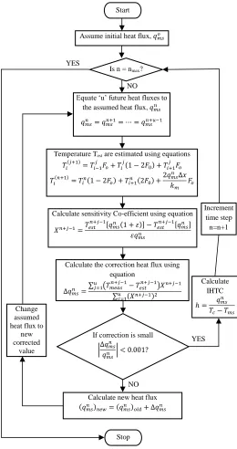
Fig. 5 Flow diagram for the estimation of IHTC by Beck’s approach
The finite difference approximation for the governing equation
at any interior node in the mould using the explicit scheme
was given in Eq. (18).
𝑇𝑖(𝑗+1)= 𝑇𝑖−1𝑗 𝐹𝑜+ 𝑇𝑖𝑗(1 − 2𝐹0) + 𝑇𝑖+1𝑗 𝐹𝑜 (18)
Eq. (18) was used for the determination of the inside nodal point temperatures of the mould for the next time step with known value of the temperature in the previous time step. The estimated temperature ‘Test’ for the calculation of sensitivity coefficient and surface heat flux was determined by the Eq. (18). The mould surface temperature for the next intermediate time step with the known values of the assumed constant heat flux and the previous time step temperature using the explicit scheme is given by Eq. (19).
n ms
q
n ms
q
2 2 T 1 T
x t
Increment time step n=n+1
Calculate IHTC
ℎ = 𝑞𝑚𝑠𝑛 𝑇𝑐− 𝑇𝑚𝑠 Equate ‘u’ future heat fluxes to
the assumed heat flux, 𝑞𝑚𝑠𝑛
𝑞𝑚𝑠𝑛 = 𝑞𝑚𝑠𝑛+1= ⋯ = 𝑞𝑚𝑠𝑛+𝑢−1
Temperature Test are estimated using equations 𝑇𝑖(𝑗+1)= 𝑇𝑖−1𝑗 𝐹
𝑜+ 𝑇𝑖𝑗(1 − 2𝐹0) + 𝑇𝑖+1𝑗 𝐹𝑜
𝑇𝑖(𝑛+1)= 𝑇𝑖𝑛(1 − 2𝐹𝑜) + 𝑇𝑖+1𝑛 (2𝐹0) +
2𝑞𝑚𝑠𝑛 ∆𝑥
𝑘𝑚 𝐹𝑜
Calculate sensitivity Co-efficient using equation
𝑋𝑛+𝑗−1=𝑇𝑒𝑠𝑡𝑛+𝑗−1[𝑞𝑚𝑠𝑛 (1 + 𝜀)] − 𝑇𝑒𝑠𝑡𝑛+𝑗−1[𝑞𝑚𝑠𝑛 ]
𝜀𝑞𝑚𝑠𝑛
Calculate the correction heat flux using equation
∆𝑞𝑚𝑠𝑛 =
∑𝑢𝑗=1 𝑇𝑚𝑒𝑎𝑠𝑛+𝑗−1− 𝑇𝑒𝑠𝑡𝑛+𝑗−1 𝑋𝑛+𝑗−1
∑𝑢 (𝑋𝑛+𝑗−1)2 𝑗=1
If correction is small
∆𝑞𝑚𝑠𝑛
𝑞𝑚𝑠𝑛 < 0.001?
Calculate new heat flux
(𝑞𝑚𝑠𝑛 )𝑛𝑒𝑤= (𝑞𝑚𝑠𝑛 )𝑜𝑙𝑑+ ∆𝑞𝑚𝑠𝑛 Change
assumed heat flux to
new corrected
value
Is n = nmax?
Start
Assume initial heat flux, 𝑞𝑚𝑠𝑜
Stop YES
NO
YES
𝑇𝑖(𝑛+1)= 𝑇𝑖𝑛(1 − 2𝐹𝑜) + 𝑇𝑖+1𝑛 (2𝐹0) +2 𝑞𝑚𝑠
𝑛 ∆𝑥
𝑘𝑚 𝐹𝑜 (19)
where ‘ i’ is the nodal point Fo is the Fourier number =
∝ ∆𝑡 𝑥2
The flow chart for the determination of surface heat flux ‘ ’ and the interfacial heat transfer coefficient for the rectangular casting using the Beck’s algorithm is given in figure 5.
6. RESULTS AND DISCUSSION
The IHTC was numerically calculated by both control volume technique and Beck’s approach for the solidification of Al alloy casting with sand mould in a rectangular geometry with the help of the measured and calculated temperatures. The experimental cast temperature variation with respect to time is shown in figure 3. During the solidification of casting it was observed that immediately after pouring, the high temperature of the cast started decreasing and at the same time, the sand mould surface temperature increased initially only for 130 seconds beyond which it started decreasing as shown in figure 3. The rise in temperature in the mould was due to the high initial thermal inertia in the mould immediately after the metal was poured in the cavity.
Fig. 6 Mould surface temperature variation estimated by Beck’s and control volume approaches
The mould surface temperature was estimated by the Beck’s approach as shown in figure 6. It is seen from the figure that four distinct stages exist during the process of solidification. In the initial period until 130 seconds the mould surface temperature falls steeply from 744oC to 479oC. The steep fall can be due to (i) the formation of small air gap between the cast and the mould inner surface (ii) the high heat absorption rate by the moulding sand due to its higher heat capacity and (iii) the presence of high temperature glide between the cast and the mould. During the second stage of solidification (130 to 340 seconds), the sudden steep fall has not been not observed. This may due to (i) low heat absorption rate of the moisture present in the sand mould (ii) The pressure exerted by the liquid metal from the riser and runner causes the solidified layer to move towards the mould wall for the directional solidification and establishes a contact with the mould surface. These two factors might be the reason for the gradual decrease in the mould surface temperature. Further, during this stage the heat flow occurred at almost constant high temperature difference maintained between the mould’s inner and outer surfaces.
The third stage of solidification was identified from 340 seconds to 460 seconds and the mould surface temperature was maintained almost constant initially and then started decreasing. The temperature difference between the mould’s inner and outer surfaces in this stage decreased.
This resulted in a decrease in the mould’s inner surface temperature, as the outer surface temperature of the mould was maintained constant. In the final stage of solidification after 460 sec to 750 sec, an almost constant temperature was seen in the entire mould inner surface. This might be due to the transfer of heat from the moulding sand to the surrounding and it was evident from the decreased experimental temperature readings after 460 seconds.
The mould surface temperature estimated from the control volume approach also had four stages similar to Beck’s algorithm but the time spans over which these trends seen were different as shown in figure 6. Both the techniques were compared for the rectangular geometry casting. The mould surface temperature calculated by Beck’s approach had higher values than the calculated values from the control volume approach for the entire time range.
Neglecting the initial high thermal inertia, the calculated temperature at the mould surface through Beck’s and Control volume approach had observable deviation which was around 46% at about 170 seconds. However, it decreased at 340 sec and it was about 15 %. Beyond 340 seconds, the difference between the mould surface temperatures calculated by two approaches reduced progressively and was almost negligible at the end of the experimentation, i.e., at about 750 seconds.
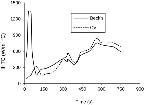
The estimated values of IHTC over time using the two different techniques are shown in figure 7. It is seen from the figure that the IHTC calculated by Beck’s approach has a higher value during the initial stage and suddenly decreases, but for the control volume approach such higher value of IHTC is not observed during the initial stage of solidification. The following reason could be identified for such a high value of IHTC by Beck’s approach. Although there is a very high heat flux at the metal mould interface, the initial presumed low value of heat flux prevails in Beck’s approach before it reaches the thermocouple. This approach overcorrects the initial assumption before the heat is conducted into the thermocouple measurement and this leads to a larger value of IHTC at the initial stage. The green sand having very low thermal diffusivity further accelerates this effect. These might be some of the reasons for the higher value of mould surface heat flux and mould surface temperature during the initial stage of solidification than the control volume approach. Neglecting the initial thermal inertia period of 130 seconds, the estimated IHTC values by Beck’s approach vary in the range of 750- 285 W/m2oC and control volume approach has a range of 840–180 W/m2 oC.
Fig. 7 IHTC variation with time estimated by Beck’s and control volume approaches
The IHTC values calculated by both techniques are almost close values for the entire duration except in the initial thermal inertia period. Disregarding this initial effect, the IHTC calculated by control volume approach has a maximum deviation of 36% at about 230 seconds from
n ms
q
0 150 300 450 600 750 900
0 150 300 450 600 750 900
M
o
ld
s
u
rf
a
c
e
t
e
m
p
e
ra
tu
re
(
ºC
)
Time (s)
Beck's
CV
0 300 600 900 1200 1500
0 150 300 450 600 750 900
IHT
C
(W
/m
2ºC)
Time (s) Beck's
Beck’s approach. The estimated IHTC values from Beck’s approach and control volume approach are closer values at the later stages of solidification and followed by the same cooling curve. Moreover, the overall trend of the IHTC plot agrees well with similar plots reported in the earlier works (Kuo et al., 2001, Woodbury et al., 2000).
7. CONCLUSIONS AND REMARKS
This work estimated and compared the mould surface temperature and IHTC for rectangular geometry aluminum alloy casting during solidification with sand mould through Beck’s and control volume approaches. The following conclusions were reached.
The calculated IHTC and mould surface temperature by Beck’s and control volume approach has almost identical trend. The results obtained by control volume approach are accurate and
reliable, and also it does not have much iteration like Beck’s approach.
A high variation of IHTC with respect to time is observed during the entire period of solidification process. This is due to the complex phenomenon of solidification and shrinkage of materials that causes varying interfacial gap between the mould and the metal surface. Hence a constant value for the heat transfer coefficient cannot be given as an input when the analysis is carried out using the commercial software used for casting process. An average heat transfer coefficient at four different stages as observed from the present work can be given as input for IHTC for the analysis.
NOMENCLATURE
∆x control volume elemental width in x direction (m) A heat flow area (m2)
b breadth of the rectangular plate (m) c specific heat (J/kg C)
Fo Fourier number
h interfacial heat transfer coefficient (W/m2C) k thermal conductivity (W/m C)
l length of the rectangular plate (m) Q heat flow (W)
q heat flux (W/m2) T temperature (C) t time (s) x distance (m) X sensitivity coefficient ε incremental value
Greek symbols
thermal diffusivity (m2/s) ρ density (kg/m3)
Superscripts j time step
u number of future time steps for which ‘qms’ is constant
Subscripts c cast
E thermocouple location at the mould est estimated
i nodal point considered ini initial
m mould mea measured ms mould surface
S thermocouple location at the surface
REFERENCES
Basil Coates, A. Stavros. Argyropoulos, 2007. “The effects of surface roughness and metal temperature on the heat transfer coefficient at the metal mold interface”, Metallurgical and Materials Transactions B, vol. 38B, pp.243-255.
Beck, J.V., Ben Blackwell, Charles, R., St. Clair, 1985. “Inverse heat conduction: Ill-Posed problem”, A Wiley-Interscience Publication, New York.
Beck, J.V., 1970. “Nonlinear estimation applied to the nonlinear inverse heat conduction problem”, International Journal of Heat Mass Transfer, vol. 13, pp.703-716. http://dx.doi.org/10.1016/0017-9310(70)90044-X
Burggraf, O.R., 1964. “An exact solution of the inverse problem in heat conduction theory and applications”, Journal of Heat Transfer, vol. 86C, pp. 373-382. https://dx.doi.org/10.1115/1.3688700
Christopher A Long, Essential heat transfer, Addison Wesley Longman (Singapore) Private Limited, Indian Branch, Delhi, 2001.
Ho, K., Pehlke, R.D., 1985. “Metal–mold interfacial heat transfer”, Metallurgical Transactions B vol.16B, pp. 585-594.
Ho, K., Pehlke, R.D., 1984. “Mechanisms of heat transfer at a metal-mold interface”, AFS Transactions, vol. 61, pp. 587-598.
Hsu, T.R., Sun, N.S., Chen, G.G., Gong, Z.L., 1992. “Finite element formulation for two-dimensional inverse heat conduction analysis”, Journal of Heat Transfer, vol.114, pp.553-557.
http://dx.doi.org/10.1115/1.2911317
Hwang, J.C., Chuang, H.T., Jong, S, H., Hwang, W.S., 1994. “Measurement of heat transfer coefficient at metal/mold interface during casting”, AFS Transactions, vol.144, pp.877-883.
Kuo, J.H., Hsu, F.L., Hwang, W.S., Yeh, J.L., Chen, S.J., 2001. “Effects of mold coating and mold material on the heat transfer coefficients at the casting/mold interface for permanent mold casting of A 356 Aluminum alloy”, AFS Transactions, vol. 61, pp.469-485.
Lau, F., Lee, W.B., Xiong, S.M., Liu, B.C., 1998. “A study of the interfacial heat transfer between an iron casting and metallic mould”, Journal of Material Processing Technology, vol. 79, pp. 25-29.
http://dx.doi.org/10.1016/S0924-0136(97)00449-4
Lazar Kovacevi, Pal Terek, Damir Kakas, Aleksandar Miletic, 2012. “A correlation to describe interfacial heat transfer coefficient during solidification of Al–Si alloy casting”, Journal of Materials Processing Technology, vol. 212, pp.1856–1861.
Lukens, M.C., Hou, T.X., Pehlke, R.D., 1990. “Mold/metal gap formation of Aluminum alloy 356 cylinders cast horizontally in dry and green sand”, AFS Transactions, vol.03, pp.63-70.
Masanori, 2000. “Analytical method in inverse heat transfer problem using Laplace Transform techniques”, International Journal of Heat and Mass Transfer, vol.43, pp. 3965-3975.
Narayan Prabhu, K., Bheemappa Chowdary, Venkatraman, N., 2005. “Casting/mold thermal contact heat transfer during solidification of Al-Cu-Si alloy (LM 21) plates thick and thin molds”, Journal of Materials Engineering and Performance, vol.14, pp.604-609.
Narayan Prabhu, K., Ravishankar, B.N., 2003. “Effect of modification melt treatment on casting/chill interfacial heat transfer and electrical conductivity of Al-13% Si alloy”, Material Science and Engineering, vol. 360, pp.293-298. http://dx.doi.org/10.1016/S0921-5093(03)00467-2
solidification in graphite-lined permanent molds”, Journal of Materials Engineering and Performance, vol.13, pp.619-626.
Rajaraman, R., Velraj, R., 2007. “Comparison of interfacial heat transfer coefficient estimated by two different techniques during solidification of cylindrical aluminum alloy casting”, HMT, vol.44, pp.1024-1034.
http://dx.doi.org/10.1007/s00231-007-0335-7
Ramesh K., Nayak and Suresh Sundarraj, 2009. “Selection of Initial Mold–Metal Interface Heat Transfer Coefficient Values in Casting Simulations—A Sensitivity Analysis” Metals & Materials Society and ASM International, vol.41B, pp.151-160
Taler, J., Zima, W., 1999. “Solution of inverse heat conduction problems using control volume approach”, International Journal of Heat and Mass Transfer, vol. 42, pp.1123-1140.
https://doi.org/10.1016/S0017-9310(98)00280-4
Vasileiou, A.N., Vosniakos, G.C., and Pantelis, D.I., 2017. “On the feasibility of determining the Heat Transfer Coefficient in casting simulations by Genetic Algorithms”, Procedia Manufacturing, vol.11, pp.509 – 516. http://dx.doi.org/10.1016/j.promfg.2017.07.144
Veerarajan, T., Ramachandran, T., 2004. “Theory and problems in numerical methods with programs in C and C++”, Tata McGraw-Hill Publishing Company Limited, New Delhi.
Woodbury, K.A., Ke, Q., Piwonka, T.S., 2000. “Mold-metal interfacial heat transfer coefficients during resin-bonded sand casting of Aluminum A356”, AFS Transactions, vol.129, pp.259-264.
Zhang, A., Liang,S., Gu, Z., Xiong,S., 2017. “Determination of the interfacial heat transfer coefficient at the metal-sand mold interface in low pressure sand casting” Experimental Thermal and Fluid Science, vol.88, pp.472–482.