Application of Model-Based Estimation to Time-Delay Estimation of Ultrasonic Testing Signals

Journal of Theoretical and Applied Vibration and Acoustics 1(1) 10-20 (2015)

* Corresponding Author: Farhang Honarvar, E-mail: [email protected]

I S A V

Journal of Theoretical and Applied

Vibration and Acoustics

journal homepage: http://tava.isav.ir

Application of Model-Based Estimation to Time-Delay Estimation of

Ultrasonic Testing Signals

Ali Gholami

, Farhang Honarvar

*, Hamid Abrishami Moghaddam

a _{Faculty of Mechanical Engineering, K.N. Toosi University of Technology, Tehran, Iran}

b _{Faculty of Electrical Engineering, K.N. Toosi University of Technology, Tehran, Iran}

K E Y W O R D S

A B S T R A C T

Ultrasonic

Time-Delay-Estimation

Model-based

SAGE algorithm

Time-Delay-Estimation (TDE) has been a topic of interest in many applications in the past few decades. The emphasis of this work is on the application of model-based estimation (MBE) for TDE of ultrasonic signals used in ultrasonic thickness gaging. Ultrasonic thickness gaging is based on precise measurement of the time difference between successive echoes which reflect back from the back wall of the test piece. The received echoes are modeled by Gaussian pulses and the desired system response is estimated using Gauss-Newton and Space Alternating Generalized Expectation Maximization (SAGE) algorithms. In addition to the model-based estimation approach, five other TDE techniques including peak-to-peak measurement, cross-correlation, cross-correlation with interpolation, phase-slope, and cross-correlation with Wiener filtering are also considered and compared with the SAGE. The main advantage of the SAGE algorithm, in addition to its higher accuracy, is its ability to deconvolve the overlapping echoes.

©2015 Iranian Society of Acoustics and Vibration, All rights reserved

1. Introduction

There is increasing interest in faster and more accurate thickness measurement techniques. One of the advanced methods used for thickness gauging is ultrasonic technique which is flexible enough to measure parts with complex shapes and different thickness ranges and materials. Some of the advantages of ultrasonic thickness gauging compared to other methods are: 1) high penetration power which allows it to measure very thick parts, 2) can be used in both contacting and non-contacting approaches (suitable for special cases like hot surfaces), 3) can be used for almost all materials from biological to metals and ceramics, 4) poses no environmental or health risks. Ultrasonic thickness gaging is usually done using the well-known pulse-echo technique (Shull 2002).

11 Another method that enables extracting ultrasonic testing echoes is Model-Based Estimation (MBE) method. (Demirli and Saniie 2001) modeled ultrasonic backscattered echoes in terms of superimposed Gaussian echoes corrupted by noise. They were able to resolve closely-spaced overlapping echoes by using space alternating generalized expectation maximization (SAGE) algorithm. Their proposed model consisted of five parameters one of which was TOF. Hajian and Honarvar (2011) applied the SAGE algorithm to signals obtained from adhesively bonded joints in order to estimate their reflectivity.

It is essential to estimate the parameters of the model accurately and quickly. (Demirli and Saniie 2001) tailored a fast Gauss Newton algorithm in order to estimate ultrasonic nondestructive testing echoes. The main shortcoming of their algorithm was its dependence on an initial guess. In order to solve this problem, Gholami et al. (2015) proposed a combined algorithm of particle swarm optimization and Gauss Newton which was independent from the initial guess to some extent. (Zhou, Zhang et al. 2015) proposed a parameter method based on artificial bee colony (ABC) algorithm which was able to estimate parameters of ultrasonic testing model accurately.

The methods used to estimate TOF in ultrasonic applications are mostly based on cross-correlation (CC). However, there are a number of shortcomings in the CC technique due to the assumptions made. In the CC technique, the received echo is realized to be a copy of the original echo with time shift, amplitude scale and noisy conditions. Therefore, CC is efficient as far as 1) the additive noise is white Gaussian noise (WGN), and 2) the received echo is a copy of the original echo with time difference and amplitude scale. Consequently, any situation that crosses these conditions would degrade accuracy of the estimated TOF. Moreover, CC cannot discriminate overlapping echoes and echoes have to be completely separated from one another (Demirli and Saniie 2001).

In this paper, we will use a model-based estimation (MBE) method for estimating the time delay of ultrasonic signals. This MBE method can be used for both non-overlapping and overlapping echoes. The method is first applied to simulated and then to measured ultrasonic testing signals and the results are compared with those obtained by the cross-correlation technique.

2. Ultrasonic thickness gaging

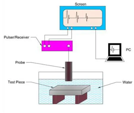
One of the applications of ultrasonic nondestructive testing is thickness measurement of industrial materials. The possibility of measuring the thickness without needing to reach both sides of a test piece makes this technique very popular. The basic principles of ultrasonic thickness gauging are as follows. A transducer transforms a voltage pulse generated by an ultrasonic pulsar into an ultrasonic pulse. The ultrasonic pulse is then sent into the test piece and when it reaches the back wall of the test piece, some part of the energy is reflected back. The reflected energy is received by the same transducer and is transformed formed into voltage and displayed on the screen. This technique is known as pulse-echo technique in which the ultrasonic probe acts as both transmitter and receiver. Immersion version of this method, in which the probe and test piece are immersed in water, is schematically shown in Figure 1.

12 The thickness of the part is determined by measuring the time it takes for the ultrasonic pulse to travel from the probe through the material to the backwall of the test piece and return back. In order to estimate the TOF between echoes more accurately, different signal processing techniques have been developed. Knowing the wave velocity of the test piece, the TOF can be directly related to the thickness as follows:

𝑐 =2𝐷

𝜏𝑑 (1)

where D is the thickness, td is travel time and c is wave velocity.

3. Model-based estimation

3.1. Gaussian echo model

In ultrasonic testing, the reflected signal from a flaw or a surface can be presented by a Gaussian model which is given as (Demirli and Saniie 2001):

𝑔(𝜃; 𝑡) = 𝛽𝑒−𝛼(𝑡−𝜏)2_{cos(2𝜋𝑓}

𝑐(𝑡 − 𝜏) + 𝜑)

𝜃 = [𝛼, 𝜏, 𝑓𝑐, 𝜑, 𝛽]

(2)

The parameters of the Gaussian echo are: α - bandwidth factor in MHz2_{, τ - arrival time in μs, fc- center frequency in}

MHz, 𝜑- phase in radians, and β = amplitude in arbitrary units. Each of these parameters represents one of the characteristics of the reflected echo. Time of arrival, τ, is related to the location of the reflector. The bandwidth factor,α, determines the bandwidth of the echo in frequency domain. The center frequency, fc, is directly related to the center frequency of the transducer. Amplitude and phase are also related to impedance, size, and orientation of the reflector (Sandell and Grennberg 1995).

In order to make the echo more realistic, the effect of noise should also be taken into account. The additive noise in this paper is white Gaussian noise (WGN). Finally, the actual echo could be presented as:

𝑥(𝑡) = 𝑔(𝜃; 𝑡) + 𝑛(𝑡) (3)

where 𝑔(𝜃; 𝑡)is a Gaussian echo and 𝑛(𝑡) is WGN.

In real ultrasonic testing signals, there are usually more than one single echo in the received signal. These echoes are reflected back from different reflectors having various sizes and being in various positions along the propagation path. By taking this point into account that each reflected echo can be modeled by a Gaussian echo, the model for M reflectors can be given as:

ℎ(𝑡) = ∑ 𝑔(𝜃𝑚, 𝑡) +

𝑀

𝑚=1

𝑛(𝑡) (4)

The parameters of each echo can be expressed as a vector 𝜃𝑚= [𝛼𝑚𝜏𝑚𝑓𝑐𝑚𝜑𝑚𝛽𝑚]. Each echo is defined completely and uniquely by its parameter vector.

3.2. Parameter estimation of a single echo

For estimating parameters of a single echo such as x, first, an objective function should be defined. Our goal is to estimate the parameter vector 𝜃 from the observation x. For doing so, we should minimize the following objective function which only uses the observed data x and the model g (θ),

13 The parameter vector which causes the Gaussian echo to nicely fit the observed echo (x) is the intended parameter vector. In other words, the parameter vector which minimizes the Mean Squares Error (MSE) between the observed echo (x) and the modeled echo (g) is the solution of this problem. This optimization problem is recognized as an unconstrained nonlinear Least Square (LS) problem. Many different algorithms can be used to solve this problem each of which may have its own pros and cons. However, in this study, due to its high speed, the Gauss Newton (GN) algorithm is used for solving this problem. GN is an iterative algorithm which works as follows:

𝜃𝑘+1= 𝜃𝑘+ (𝐻(𝜃𝑘)𝐻(𝜃𝑘))

−1

𝐻𝑇_(𝜃

𝑘)(𝑥 − 𝑠(𝜃𝑘)) (6)

Where k is the count of iteration and H(θ) is the gradient of the model given by:

𝐻(𝜃) = [𝑑𝑠(𝜃)

𝑑𝛼 𝑑𝑠(𝜃)

𝑑𝜏

𝑑𝑠(𝜃)

𝑑𝑓𝑐

𝑑𝑠(𝜃) 𝑑𝜑

𝑑𝑠(𝜃)

𝑑𝛽 ] (7)

For estimating this gradient matrix, both numerical and analytical methods can be used. However, to increase the speed of the computation, the analytical method is used. To facilitate the computation process, the following two kernel functions are introduced:

𝑓(𝜃) = 𝑒−𝛼(𝑡−𝜏)2_{cos{2𝜋𝑓}

𝑐(𝑡 − 𝜏) + 𝜑}

(8)

𝑔(𝜃) = 𝑒−𝛼(𝑡−𝜏)2

sin{2𝜋𝑓𝑐(𝑡 − 𝜏) + 𝜑}

The analytical derivatives are calculated as:

𝑑𝑠(𝜃)

𝑑𝛼 = −𝛽(𝑡 − 𝜏)2𝑓(𝜃)

(9)

𝑑𝑠(𝜃)

𝑑𝑓𝑐 = −2𝜋𝛽(𝑡 − 𝜏)𝑔(𝜃)

𝑑𝑠(𝜃)

𝑑𝑡 = −2𝛼(𝑡 − 𝜏)𝑓(𝜃) + 2𝜋𝑓𝑐𝛽𝑔(𝜃)

𝑑𝑠(𝜃)

𝑑𝜑 = −𝛽𝑔(𝜃)

𝑑𝑠(𝜃)

𝑑𝛽 = 𝑓(𝜃)

The algorithm will keep computing gradient vectors in each iteration till the improvement in the parameter vectors is smaller than a predefined tolerance. The GN algorithm for parameter estimation of a Gaussian echo can be implemented in the following computational steps:

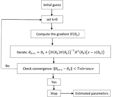
Step 1. Make an initial guess for the parameter vector 𝜃 (0) and set k=0 (iteration number).

Step 2. Compute the gradients 𝐻(𝜃(𝑘)) and the model 𝑠(𝜃(𝑘))

.

Step 3. Iterate the parameter vector: 𝜃(𝑘 + 1) = 𝜃(𝑘) + (𝐻𝑇 (𝜃(𝑘))𝐻(𝜃(𝑘)))− 1𝐻𝑇 (𝜃(𝑘))(𝑥 − 𝑠(𝜃(𝑘)))

.

Step 4. Check convergence criterion: If ‖𝜃(𝑘 + 1) -𝜃(𝑘)‖ <tolerance, then stop.

Step 5. Set 𝑘 → 𝑘 + 1 and go to Step 2.

14

Fig 2: The flowchart of the GN algorithm used for estimating parameter vector of ultrasonic echoes

3.3. Parameter estimation of multiple echoes

In the previous section, the parameters of a single echo were estimated. In this section the parameter vectors of multiple echoes will be estimated. Estimating M parameter vectors is more sophisticated and more time consuming than estimating the parameter vector of a single echo. The direct LS approach to this problem requires the minimization of the following term:

‖ℎ(𝑡) − ∑ 𝑔(𝜃𝑚)

𝑀

𝑚=1

‖ 2

(10)

Where h(t) is the observed signal consisting of M Gaussian echoes. In this M dimensional optimization problem, M parameter vectors should be optimized. It means that for a signal consisting of three echoes, the algorithm should optimize 15 parameters which is not an easy task and it is very likely that the algorithm could not converge. As an alternative way, the expectation Maximization (EM) algorithm can be used; however, the EM algorithm suffers from low speed. In order to increase the speed of the EM algorithm, the Space Alternating Generalized EM (SAGE) algorithm can be used to overcome the aforementioned problem. An ultrasonic signal consisting of M unobserved Gaussian echoes can be written as:

ℎ(𝑡) = ∑ 𝑥𝑚

𝑀

𝑚=1

(11)

Where, 𝑥_𝑚 is an unobserved echo and h(t)is the ultrasonic signal. 𝑥_𝑚Cannot be directly estimated and instead its expectation is used to play its role. The expectation of 𝑥𝑚 is estimated as follows (This step is known as E-Step) (Feder and Weinstein 1988):

𝑥̂𝑚(𝑘)(𝑡) = 𝑔(𝜃𝑚(𝑘); 𝑡) +

1

𝑀[ℎ(𝑡) − ∑ 𝑔(𝜃𝑖(𝑘); 𝑡)

𝑀

𝑚=1

] (12)

Now in order to find the parameter vector of 𝑥̂

,

𝜃𝑚(𝑘+1)= 𝑎𝑟𝑔𝜃𝑚𝑚𝑖𝑛‖𝑥̂𝑚

(𝑘)_{− 𝑔(𝜃}

𝑚; 𝑡)‖

2

15 The GN algorithm is now used for solving this problem. This algorithm will be repeated for each of the M-superimposed echoes till all parameters are appropriately estimated. In summary, the SAGE algorithm for parameters Imation of M-superimposed Gaussian echoes with WGN can be implemented through the following steps:

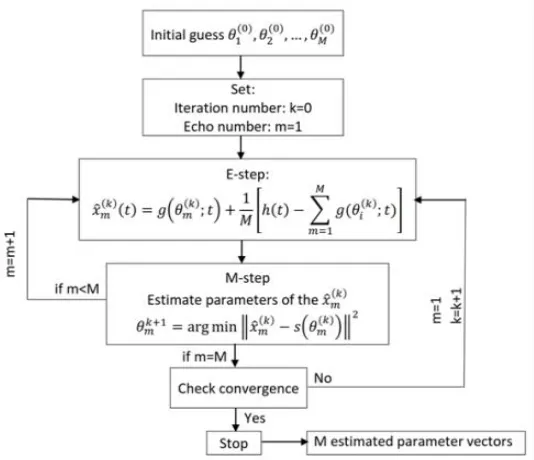
Step 1. Make initial guesses for the parameter vectors and form

𝜃

number) and m = 1 (echo number).

Step 2. Compute the expected signal for the 𝑚th echo (E-Step):

𝑥̂𝑚(𝑘)= 𝑔(𝜃𝑚(𝐾)) +

1

𝑀{ℎ(𝑡) − ∑ 𝑔(𝜃𝐿(𝐾))

𝑀

𝑙=1

}

Step 3. Iterate the 𝑚th parameter vector (M-Step): 𝜃_𝑚(𝑘+1)= 𝑎𝑟𝑔𝜃_𝑚𝑚𝑖𝑛‖𝑥̂𝑚(𝑘)− 𝑔(𝜃𝑚)‖

2

, and set 𝜃_𝑚(𝑘)= 𝜃_𝑚(𝑘+1)

Step 4. Set 𝑚 → 𝑚 + 1 and go to Step 2 unless 𝑚 > 𝑀.

Step 5. Check convergence criterion: If ‖𝜃(𝑘+1)− 𝜃(𝑘)‖ < tolerance, then stop.

Step 6. Set 𝑚 = 1, 𝑘 → 𝑘 + 1, and go to Step 2.

The flowchart of the SAGE algorithm is given in Figure 3:

Fig 3: The flowchart of the SAGE algorithm used for multiples echoes

4. Simulated ultrasonic signal

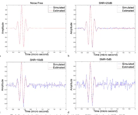
In order to examine the performance of the GN algorithm, a simulated ultrasonic signal including one single echo is used. The parameters of this echo are estimated by the GN algorithm. The parameters of the assumed echo are as follows: bandwidth factor 𝛼= 55 (MHz)2, arrival time 𝜏= 0.5 μs, center frequency 𝑓𝑐 = 7 MHz, phase φ = 0.5 rad, and amplitude 𝛽= 1. The GN algorithm needs an initial guess to start. The initial guess for this echo was

[𝛼 𝜏 𝑓 𝜑 𝛽] = [25 0.8 4 2 0.5]. The algorithm was tested with different levels of signal-to noise-ratio (SNR)

16

Table 1: Estimated and real parameters of the simulated echoes

According to the obtained results, the GN algorithm has succeeded in estimating the parameter vector of the simulated echo in all four situations with the same imputed initial guess. The SAGE algorithm was then tested on some simulated multiple Gaussian echoes. Three non-overlapping echoes and three overlapping echoes having a SNR of 10 dB were used for this purpose, see Figure 5.

a b

c d

Fig 4: Simulated echo (blue) and estimated echo (red) with different SNR’s.a) Noise free, b) SNR = 20dB,

c) SNR = 10 dB, d) SNR = 5 dB. Bandwidth

factor (MHz2)

Arrival time (μs)

Center frequency (MHz)

Phase

(rad) Amplitude

Mean square error

Actual parameters 55 0.5 7 2 1

Initial guess 25 0.8 4 2 0.5

Estimated parameters

Noise free 55.0002 0.5000 7.0000 -5.7832 1 6.0519× 10−12

SNR=20dB 54.7797 0.5011 6.9979 -5.7367 1.0053 3.3734× 10−4

SNR=10dB 50.1188 0.5020 6.9652 -5.6884 0.9470 0.0041

17

Fig 5: Estimating the parameters of a) the three non-overlapping echoes with SNR = 10 dB,

and (b) the three overlapping echoes with SNR = 10 dB.

The SAGE algorithm was used to extract the parameter vectors of these simulated echoes. Similar to estimating the parameter vector of a single echo, an initial guess is needed to be introduced to the SAGE algorithm. The initial guess, the simulated and estimated parameter vectors, and the corresponding MSE of these three non-overlapping echoes are given in Table 2.

Table2: Estimated parameters of three non-overlapping echoes with SNR of 10dB

Echo parameter Bandwidth factor

(MHz2)

Arrival time (μs)

Center frequency (MHz)

Phase (rad) Amplitude

Actual parameters 55 1 9 0 1

82 2 10 1 0.8

100 4 11 2 0.6

Initial guess 10 0.5 7 0 0.5

10 2.5 7 0 0.5

10 3.5 7 0 0.5

Estimated parameters 50.6218 1.0006 8.9647 25.1556 0.9689

82.7104 1.9969 10.0222 -24.3221 0.8428

103.6489 3.9991 10.9204 20.7990 0.5945

Similar data for the three overlapping echoes are tabulated in Table 3.

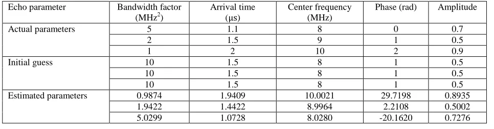
Table 3: Estimated parameters of three overlapping echoes with SNR of 10dB

Echo parameter Bandwidth factor

(MHz2)

Arrival time (μs)

Center frequency (MHz)

Phase (rad) Amplitude

Actual parameters 5 1.1 8 0 0.7

2 1.5 9 1 0.5

1 2 10 2 0.9

Initial guess 10 1.5 8 1 0.5

10 1.5 8 1 0.5

10 1.5 8 1 0.5

Estimated parameters 0.9874 1.9409 10.0021 29.7198 0.8935

1.9422 1.4422 8.9964 2.2108 0.5002

18 In Figure 5, the SAGE algorithm was able to estimate the parameters of both the overlapping and non-overlapping echoes. The mean square errors between the estimated and simulated echoes were 0.003 for non-overlapping echoes

and 0.0175 for overlapping echoes. The main advantage of the SAGE algorithm is its ability to discriminate the

overlapping echoes.

5. Measured ultrasonic signal

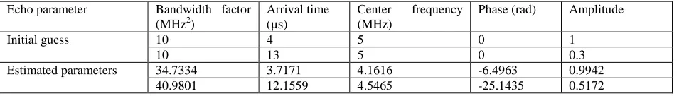
In this Section, first, a single ultrasonic echo is measured by using the pulse-echo ultrasonic testing technique. This is a back wall echo received from a 20 mm thick steel block tested by a 4 MHz ultrasonic probe. The measured echoes sampled at 100 MHz with a resolution of 12 bit. The initial guess was [𝛼 𝜏 𝑓 𝜑 𝛽] = [35 0.6 3.5 20.5]. The measured echo and its corresponding estimated echo are shown in Figure 6. The estimated parameter vector is also tabulated in Table 4.The results given in Figure 6 and Table 4 show that the GN algorithm has been able to successfully and accurately reconstruct the measured echo. In the next experiment, two consecutive back wall echoes of the same steel block are analysed by using the SAGE algorithm. All settings are the same as the first experiment. The acquired signal is shown in Figure 7. Along with its corresponding model-based estimated signal. The model obtained for this signal is a good match with a mean square error of 2.8869 × 10−4. The estimated time-of-arrival betwean the two echoes is 8.4388 μs.This signal is also examined by five other time delay estimation (TDE) methods. These five methods are: peak-to-peak, cross-correlation (CC), CC-interpolation, phase slope and CC-Wiener. The estimated times are tabulated in Table 5. Comparison of the results reported in Table 5 shows that the SAGE algorithm has been able to estimate the time delay pretty accurately.

Fig 6: A single experimental echo (blue) and its corresponding Gaussian echo estimated by the GN algorithm (red)

Table 4: Initial guess and estimated parameters of the measured signal

Echo parameter Bandwidth factor (MHz2)

Arrival time (μs)

Center frequency (MHz)

Phase (rad) Amplitude

Initial guess 10 4 5 0 1

10 13 5 0 0.3

Estimated parameters 34.7334 3.7171 4.1616 -6.4963 0.9942

40.9801 12.1559 4.5465 -25.1435 0.5172

0 0.1 0.2 0.3 0.4 0.5 0.6 0.7 0.8 0.9 1 -1

-0.8 -0.6 -0.4 -0.2 0 0.2 0.4 0.6 0.8 1

Time (micro second)

A

m

pl

it

ude

19

Fig7: Measured (blue) and estimated (red) echoes obtained from a 20 mm thick steel block

Table 5: TOF of the experimental signal measured by different methods

CC-Wiener Phase slope

CC-interpolation Cross correlation

Peak to peak TDE method

8.4328378 8.4484485

8.4326911 8.43

8.43 TOF (μs)

In addition to time delay estimation capability of the SAGE algorithm, it can also extract other valuable information from ultrasonic echoes such as frequency and phase each of which reveals some momentous characteristics of the test piece. Moreover, the SAGE algorithm can be used for discriminating echoes which have overlapped and this is very useful in ultrasonic testing of thin layers.

6. Conclusion

In this study, we used a model-based estimation method for analysis and system identification of ultrasonic back scattered echoes. The method is based on the Gaussian echo model whose parameters represent certain signal characteristics (TOF, bandwidth, frequency, phase, and amplitude) of an ultrasonic echo. The received echoes can be represented by a sum of Gaussian echoes whose parameters are accurately estimated. The SAGE algorithm was then applied to both overlapping and non-overlapping simulated echoes. The algorithm was also applied to a real ultrasonic signal and its parameters were estimated. The TOF measured by the SAGE algorithm was compared with other TDE techniques and showed to be in good agreement with them. By using the SAGE algorithm, not only can the TOF between two echoes be measured, but also other characteristics of the signal are identified. Another advantage of the SAGE algorithm over other methods is its ability to estimate overlapping echoes, while other methods do not have such capability. Because of this advantage, it can be used for testing thin sheets as well as adhesively bonded joints whose back wall echoes usually overlap.

References

1 . Demirli, R. and J. Saniie, Model-based estimation of ultrasonic echoes. Part I: Analysis and algorithms. Ultrasonic, Ferroelectrics and Frequency Control, IEEE Transactions on 48(3) (2001)787-802.

20 3 .Feder, M. and E. Weinstein), Parameter estimation of superimposed signals using the EM algorithm. Acoustics, Speech and Signal Processing, IEEE Transactions on 36(4) (1988) 477-489.

4 .Jacovitti, G. and G. Scarano, Discrete time techniques for time delay estimation. Signal Processing, IEEE Transactions on 41(2) (1993) 525-533.

5 .Matz, V, R. Smid, S, Starman and M. Kreidl , Signal-to-noise ratio enhancement based on wavelet filtering in ultrasonic testing. Ultrasonics 49(8) (2009) 752-759.

6 .Sandell, M. and A. Grennberg , Estimation of the spatial impulse response of an ultrasonic transducer using a tomographic approach. The Journal of the Acoustical Society of America 98(4) (1995) 2094-2103.

7 .Shull, P. J, Nondestructive evaluation: theory, techniques, and applications, CRC press, (2002).

8 .Zhou, J., X. Zhang, G. Zhang and D. Chen , Optimization and Parameters Estimation in Ultrasonic Echo Problems Using Modified Artificial Bee Colony Algorithm. Journal of Bionic Engineering 12(1) (2015)160-169. 9 .F. Honarvar, F. Salehi, V. Safavi, A. Mokhtari, and A. N. Sinclair, Ultrasonic monitoring of erosion/corrosion thinning rates in industrial piping systems, Ultrasonics, vol. 53(2013)1251-1258.

10 .F. Honarvar, M. Iran-Nejad, A. Gholami, and A. Sinclair, Estimation of Uncertainty in Ultrasonic Thickness Gauging and Improvement of Measurements by Signal Processing, in Annual Conference, ed. Toronto, Canada: Canadian Institute of Nondestructive Evaluation (CINDE), 2014.

11 .M. Hajian and F. Honarvar, Reflectivity Estimation using an Expectation Maximization Algorithm for Ultrasonic Testing of Adhesive Bonds, Materials Evaluation, 2011.