Combining Unsupervised and Supervised
Classification to Build User Models for Exploratory
Learning Environments
SALEEMA AMERSHI
[email protected], University of Washington and
CRISTINA CONATI
[email protected], University of British Columbia
________________________________________________________________________
In this paper, we present a data-based user modeling framework that uses both unsupervised and supervised classification to build student models for exploratory learning environments. We apply the framework to build student models for two different learning environments and using two different data sources (logged interface and eye-tracking data). Despite limitations due to the size of our datasets, we provide initial evidence that the framework can automatically identify meaningful student interaction behaviors and can be used to build user models for the online classification of new student behaviors online. We also show framework transferability across applications and data types.
Keywords: Data Mining, Unsupervised and Supervised Classification, User Modeling, Intelligent Learning Environments, Exploratory Learning Environments
________________________________________________________________________
1. INTRODUCTION
Exploratory learning environments (ELEs from now on) are educational tools designed to foster learning by supporting students in freely exploring relevant instructional material (often including interactive simulations), as opposed to relying on structured, explicit instruction as with more traditional intelligent tutoring systems (ITS) [Shute and Glaser 1990]. In theory, this type of active learning should enable students to acquire a deeper, more structured understanding of concepts in the domain [Piaget 1954; Ben-Ari 1998]. In practice, empirical evaluations have shown that ELEs are not always effective for all students (e.g. [Shute 1993]) and that some students may benefit from more structured support [Kirschner et al. 2006].
Merten and Conati [2007] have also explored an approach based on supervised machine learning, where domain experts manually labeled interaction episodes based on whether students reflected or not on the outcome of their exploratory actions. The resulting data set was then used to train a classifier for student reflection behavior that was integrated with a previously developed knowledge-based model of student exploratory behavior. While the addition of the classifier significantly improved model accuracy, this approach suffers from the same drawbacks of knowledge based-approaches described earlier. It is time-consuming and error prone, because humans have to supply the labels for the dataset, and it needs a priori definitions of relevant behaviors when there is limited knowledge of what these behaviors may be.
In this paper we explore a more lightweight approach: a user modeling framework that addresses the above limitations by relying on data mining to automatically identify common interaction behaviors and then using these behaviors to train a user model. The key distinction between our modeling approach and knowledge-based or supervised approaches with hand-labeled data is that human intervention is delayed until after a data mining algorithm has automatically identified behavioral patterns. That is, instead of having to observe individual student behaviors in search of meaningful patterns to model or to input to a supervised classifier, the developer is automatically presented with a picture of common behavioral patterns that can then be analyzed in terms of learning effects. Expert effort is potentially reduced further by using supervised learning to build the user model from the identified patterns. While these models may not be as fine-grained as those generated by more laborious approaches based on expert knowledge or labeled data (e.g., they recognize classes of behaviors as opposed to more specific behaviors), they may still provide enough information to inform soft forms of adaptivity in-line with the unstructured nature of the interaction with ELEs. One potential problem of this approach is that it requires a substantial amount of data to work and collecting this data can be time-consuming. This is true, for instance, if the data is collected during laboratory studies, as was the case for the two experiments that we describe in this paper. However, since behavioral patterns also manifest themselves in normal usage of a target system, it is possible that data could be obtained from an uncontrolled setting, making data availability less of an issue, especially if the system is made available online.
automatically used in student modeling. The work presented in this paper contributes to both these areas. First, most of the work on EDM has focused on traditional intelligent tutoring systems that support structured problem solving (e.g., [Sison et al 2000; Zaiane 2002; Baker et al. 2008]) or drill and practice activities (e.g. [Beck 2005]), where students receive feedback and hints based on the correctness of their answers. In contrast, our work aims to model students as they interact with environments that support learning via exploratory activities like interactive simulations, where there is no clear notion of correct or incorrect behavior. We show that by applying unsupervised clustering to log data, we identify interaction patterns that are meaningful to discriminate different types of learners and that would be hard to detect based on intuition or basic correlation analysis. Second, most existing approaches have been tested within a single ITS (although Baker et al. [2008] have shown transferability across different lessons within the same ITS). In contrast, we show the effectiveness of our approach applied to two different ELEs (the AIspace Constraint Satisfaction Problem (CSP) Applet [Amershi et al. 2005] and the Adaptive Coach for Exploration (ACE) learning environment [Bunt et al. 2001]) and to two different types of data, one involving interface actions only and another involving both interface actions and eye-tracking data. We obtained comparable results in our experiments, demonstrating that our user modeling framework can be applied to different applications and data types.
It was our initial work with the CSP Applet (described in [Amershi and Conati 2006]) that gave us the idea of devising a framework to generalize the approach we used in that experiment. The framework and its application to the ACE learning environment has been discussed in [Amershi and Conati 2007], along with a brief comparison with the work on the CSP Applet. In this paper we present a unified view of this work. In particular, we updated the work on the CSP Applet to be in line with the framework formalized in [Amershi and Conati 2007]. We also provide an extended comparison of our two experiments which is important for demonstrating framework transferability.
2. USER MODELING FRAMEWORK
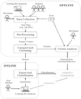
Fig. 1. User modeling framework. The adaptive component based on the model created by the framework is itself outside of the framework (and therefore appears grayed out in the figure).
In the next two sections (Sections 2.1 and 2.2), we detail the two phases supported by the framework, including describing the algorithms we chose to complete these phases. Then in Section 2.3 we explain how we evaluate the user models that we developed for both of our experiments (see Sections 3 and 4).
2.1 Offline Identification
This phase uses unsupervised machine learning to automatically identify distinct student interaction behaviors in unlabeled data. The rest of this section describes the different steps of the offline phase, outlined at the top of Figure 1.
catalog) of all possible primitive interaction events that can occur in the environment so that they can be logged (see the solid arrow from ‘Developer’ to ‘Data Collection’ in Figure 1). In addition to interface actions, logged data can include events from any other data source that may help reveal meaningful behavioral patterns (e.g., an eye-tracker).
An additional form of data to collect is tests on student domain knowledge before and after using the learning environment (sees the dotted arrow in Figure 1 from ‘Tests’ to ‘Data Collection’). The purpose of these tests is to measure student learning with the system to facilitate the cluster analysis step, as we will see below.
Preprocessing. Clustering operates on data points in a feature space, where features can be any measurable property of the data [Jain et al. 1999]. Therefore, in order to find clusters of students who interact with a learning environment in similar ways, each student must be represented by a multidimensional data point or ‘feature vector’. The second step in the offline phase is to generate these feature vectors by computing low level features from the data collected. We suggest features including (a) the frequency of each interface action, and (b) the mean and standard deviation of the latency between actions. The latency dimensions are intended to measure the average time a student spends reflecting on action results, as well as the general tendency for reflection (e.g., consistently rushing through actions vs. selectively attending to the results of actions). We use these features in both of our experiments (see Sections 3 and 4). In our second experiment, we also include features extracted from eye-tracking data (i.e., eye gaze movements) to demonstrate that our approach works with a variety of input sources.
manual feature selection, in our second experiment we employ an entropy-based unsupervised feature selection algorithm presented in [Dash and Liu 2000].
Unsupervised Clustering. After forming feature vector representations of the data, the next step in the offline phase is to perform clustering on the feature vectors to discover patterns in the students’ interaction behaviors. Clustering works by grouping feature vectors by their similarity, where here we define similarity to be the Euclidean distance between feature vectors in the normalized feature space.
We chose the well-known partition-based k-means [Duda et al. 2001] clustering algorithm for this step in both of our experiments. While there exists numerous clustering algorithms (see [Jain et al. 1999] for a survey) each with its own advantages/disadvantages, we chose k-means as proof-of-concept because of its simplicity. Furthermore, the k-means algorithm scales up well because its time complexity is linear in the number of feature vectors.
K-means converges to different local optima depending on the selection of the initial
cluster centroids and so in this research we execute 20 trials (with randomly selected initial cluster centroids) and use the highest quality clusters as the final cluster set. We measure quality based on Fisher’s criterion [Fisher 1936] in discriminant analysis which reflects the ratio of between to within-cluster scatter. That is, high quality clusters are defined as having maximum between-cluster variance and minimum within-cluster variance.
The second step in cluster analysis is to explicitly characterize the interaction behaviors in the different clusters by evaluating cluster similarities and dissimilarities along each of the feature dimensions. While this step is not strictly necessary for online user recognition based on supervised classification (see Section 2.2), it is useful to help educators and developers gain insights on the different learning behaviors and devise appropriate adaptive interventions targeting them.
In this research, we use formal statistical tests to compare clusters in terms of learning and feature similarity. For measuring statistical significance, we use Welch’s t-test for unequal sample variances when comparing two clusters, and one-way analysis of variances (ANOVAs) with Tukey HSD adjustments (pHSD) for post-hoc pair-wise comparison [Faraway 2002] to compare multiple clusters. To compute effect size (a measure of the practical significance of a difference) with use Cohens’s d [Cohen 1988] for two clusters (where d > .8 is considered a large effect, and d between .5 and .8 is a
medium effect). For multiple clusters, we use partial eta-squared (partial η2) [Cohen
1988; Olejnik and Algina 2000], (where partial η2 > .14 is considered a large effect, and a value between .06 and .14 is a medium effect).
2.2 Online Recognition
2.3 Model Evaluation
In both of our experiments (see Sections 3 and 4) we performed an N fold leave-one-out cross validation (LOOCV) to evaluate the corresponding user models. Here we describe this evaluation method.
In each fold, we removed one student’s data from the set of N available feature vectors, and used k-means to re-cluster the reduced feature vector set (Section 2.1). Next, the removed student’s data (the test data) was fed into a classifier user model trained on the reduced set (Section 2.2), and online predictions were made for the incoming actions as described in Section 2.2. Model accuracy is evaluated by checking after every action whether the current student is correctly classified into the cluster to which he/she was assigned in the offline phase. Aggregate model accuracy is reported as the percentage of students correctly classified as a function of the number of actions seen by the classifier.
It should be noted, however, that by using a LOOCV strategy, we run the risk of altering the original clusters detected in the offline phase (offline clusters from now on) by using the entire feature vector set. Therefore, we should not expect to achieve 100% accuracy even after seeing all the actions because the user models are classifying incoming test data given the clusters found by LOOCV using the reduced set of feature vectors. In supervised machine learning, this issue is known as hypothesis stability [Kearns and Ron 1997]. In [Lange et al. 2003] the authors extend this notion to the unsupervised setting by defining a stability cost (SC), or expected empirical risk, which essentially quantifies the inconsistency between the original clusters and those produced by LOOCV. Perfect stability (SC=0) occurs when the offline clusters are unchanged by LOOCV. Conversely, maximum instability (SC=1) occurs when none of the original data labels (as defined by the original offline clusters) are maintained by LOOCV. In other words, a low SC helps to ensure that the offline clusters are relatively resistant to distortions caused by the removal of one feature vector. We compute the stability cost prior to assessing predictive accuracy to ensure that the models are essentially predicting what we would like them to predict, i.e., the membership of the removed student’s behavioral patterns in one of the offline clusters.
classification after a given number of actions and the student’s actual learning performance up to that point. One way to determine the latter is to manually label every partial sequence of student action as pedagogically effective or ineffective. However, such manual labeling is precisely what we are trying to avoid with our modeling framework.
3. TESTING THE FRAMEWORK ON THE AISPACE CSP APPLET LEARNING
ENVIRONMENT
Our first attempt at applying our user modeling framework is with an exploratory learning environment called the AIspace Constraint Satisfaction Problem (CSP) Applet. The CSP Applet is part of AIspace, a collection of interactive tools that use algorithm visualization (AV) to help students explore the dynamics common Artificial Intelligence (AI) algorithms (including algorithms for search, machine learning, and reasoning under uncertainty) [Amershi et al. 2005]. As for exploratory learning environments in general, there is evidence that the pedagogical impact of AVs depends upon how students use the tool, which in turns is influenced by distinguishing characteristics such as learning abilities and styles [Hundhausen et al. 2002; Stern et al. 2005]. Such reports emphasize the need for environments that use interactive AVs to provide adaptive support for individual students.
Here, we first describe the CSP Applet interface (Section 3.1). In Section 3.2 we describe how we applied the offline component of our framework to identity meaningful clusters of students. In Section 3.3 we apply the online component of our framework to build classifier user models for the CSP Applet and then evaluate them.
3.1 The AIspace CSP Applet Learning Environment
A CSP consists of a set of variables, variable domains and a set of constraints on legal variable-value assignments. The goal is to find an assignment of values to variables that satisfies all constraints. A CSP can be naturally represented as a graph where nodes are the variables of interest and constraints are defined by arcs between the corresponding nodes.
there are variables left with more than one domain value, a procedure called domain splitting can be applied to any of these variables to split the CSP into disjoint cases, so
that AC-3 can recursively solve each resulting case.
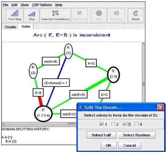
Figure 2 shows a sample CSP as it is graphically represented in the CSP Applet. Initially, all the arcs in the network are colored blue indicating that they need to be tested for consistency. As the AC-3 algorithm runs, state changes in the graph are represented via the use of color and highlighting. The CSP Applet provides several mechanisms for the interactive execution of the AC-3 algorithm, accessible through the button toolbar shown at the top of Figure 2, or through direct manipulation of graph elements. Note that the applet also provides functionalities for creating CSP networks, but in this research we limit our analysis to only those relevant to solving a predefined CSP. Here we provide a brief description of these functionalities necessary to understand the results of applying our user modeling framework to this environment.
• Fine Step. Allows the student to manually advance through the AC-3 algorithm at a
fine scale. Fine Step cycles through three stages, triggered by consecutive clicks of the Fine Step button. First, the CSP Applet selects one of the existing blue (untested) arcs and highlights it. Second, the arc is tested for consistency. If the arc is consistent, its color will change to green and the Fine Step cycle terminates. Otherwise, its color changes to red and a third Fine Step is needed. In this final stage, the CSP Applet removes the inconsistency by reducing the domain of one of the variables involved in the constraint, and turns the arc green. Because other arcs connected to the reduced variable may have become inconsistent as a result of this step, they must be retested and thus are turned back to blue. The effect of each Fine Step is reinforced explicitly in text through a panel above the graph (see message above the CSP in Figure 2).
• Step. Executes the AC-3 algorithm in coarser detail. One Step performs all three
stages of Fine Step at once, on a blue arc chosen by the algorithm.
• Direct Arc Click. Allows the student to choose which arc to Step on by clicking
directly on it.
• Domain Split. Allows a student to divide the network into smaller sub-problems by
Fig. 2. AIspace CSP Applet interface
• Backtrack. Recovers the alternate sub-problem set aside by Domain Splitting
allowing for recursive application of AC-3.
• Auto Arc Consistency (Auto AC). Automatically Fine Steps through the CSP
network, at a user specified speed, until it is consistent.
• Auto Solve. Iterates between Fine Stepping to reach graph consistency and
automatically Domain Splitting until a solution is found.
• Stop. Lets the student stop execution of Auto AC or Auto Solve at any time.
• Reset. Restores the CSP to its initial state so that the student can re-examine the
initial problem and restart the algorithm.
3.2 Offline Identification for the CSP Applet
In this section, we describe how we applied the offline steps of our proposed framework to generate user models for the AIspace Applet.
3.2.1 From Data Collection to Unsupervised Clustering for the CSP Applet
undergraduate computer science and engineering students participated in the user study. These students had sufficient background knowledge to learn about CSPs, but had no previous exposure to AI algorithms.
The study typified a scenario in which a student learns about a set of target concepts from text-based materials, studies relevant sample problems, and finally is tested on the target concepts. First, students had one hour to read a textbook chapter on CSP problems [Poole et al., 1998]. Next, they took a 20 minute test on the material. After the pre-test, students studied sample problems using the CSP Applet and finally they were given a post-test almost identical to the pre-test except for a few different domain values or arcs.
For the current experiment, we used the time-stamped logged data of user interactions with the CSP Applet, and results from the pre and post tests. From the logged data we obtained 1931 user actions over 205.3 minutes. It should be noted that we had disabled the Step and Auto Solve mechanisms for this previous user study, because we observed students misusing them during pilot studies (e.g., hastily Stepping through the problem or inattentively Auto Solving the problem). Thus, the actions included in the log files were limited to Fine Step, Direct Arc Click, Auto Arc Consistency (Auto AC), Stop Reset, Domain Split and Backtrack. While it would have been useful to see if our modeling approach could capture the misuse of Step and Auto Solve, remarkably it was still able to identify several other behaviors potentially detrimental for learning (as we discuss below). The fact that our approach discovered suboptimal learning behaviors that we could not catch by observing the interactions highlights how difficult it can be to recognize distinct learning behaviors in this type of environment.
Preprocessing. From the logged user study data, we computed 24 feature vectors corresponding to the 24 study participants. The feature vectors had 21 dimensions, resulting from deriving three features for each of the seven actions described in the previous sections: (1) action frequency, (2) the average latency after the action, and (3) the standard deviation of the latency after the action. Recall from Section 2.1 that we use the second dimension as a possible indicator of student reflection, and the third dimension as a possible indicator of selectiveness since varied latency may indicate planned rather than impulsive or inattentive behavior (as found, for instance, by Shih, Koedinger and Scheines [2008]).
we decided not to perform the feature selection step (Section 2.1) for this experiment because the number of feature dimensions was still lower than the number of feature vectors. We will see below that our framework was still able to find several meaningful behavioral patterns from the CSP Applet data.
Unsupervised Clustering. We applied k-means clustering to the study data with k set to 2, 3 and 4 because we only expected to find a few distinct clusters with our small sample size. As described in Section 2.1, for each trial we executed k-means 20 times and used the highest quality clusters as the final cluster set. The clusters found by k set to 4 were the same as those with k set to 3 with the exception of one data point forming a singleton cluster. This essentially corresponds to an outlier in the data, and so we report only the results for k set to 2 and k set to 3. We now discuss cluster analysis for k set to 2 and k set to 3, in turn.
3.2.2 Cluster Analysis for the CSP Applet (k=2)
When we compared average learning gains between the clusters found by k-means with k set to 2 (k-2 clusters from now on), we found that one cluster (4 students) had (statistically and practically) significantly (p<.05 and d>.8, respectively) higher learning gains (average=7 points, SD=2.68) than the other cluster (20 students, average=3.08 points gain, SD=2.62). Hereafter, we will refer to these clusters as ‘HL’ (high learning) cluster, and ‘LL’ (low learning) cluster respectively.
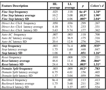
Table I. Pair-wise feature comparisons between HL and LL clusters for k = 2
Feature Description HL
average
LL
average p Cohen’s d
Fine Step frequency .025 .118 6e-4* 1.34*
Fine Step latency average 10.2 3.08 .013* 1.90*
Fine Step latency SD 12.2 4.06 .005* 2.04*
Direct Arc Click frequency .050 .036 .299 .267 Direct Arc Click latency average 4.18 5.71 .233 .331
Direct Arc Click latency SD 3.63 5.74 .177 .362
Auto AC frequency .007 .003 .118 .700
Auto AC latency average 23.7 36.9 .175 .316 Auto AC latency SD 20.4 12.8 .276 .294
Stop frequency .003 7e-4 .058 .935*
Stop latency average 1.75 1.60 .448 .047
Stop latency SD 1.06 0 .051 1.16*
Reset frequency .010 .008 .329 .221
Reset latency average 46.6 11.4 .086 .866*
Reset latency SD 24.4 9.56 .003* 1.51*
Domain Split frequency .003 .009 .012* .783
Domain Split latency average 6.75 4.61 .156 .465 Domain Split latency SD 1.37 3.04 .059 .596
Backtrack frequency 8e-4 .002 .113 .413 Backtrack latency average 1.75 3.68 .211 .281
Backtrack latency SD 0 3.27 .057 .524 * Significant at p<.05 or d>.8 (feature description and values in bold)
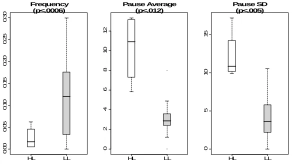
HL LL 0. 00 0. 05 0 .10 0 .1 5 0. 2 0 0. 25 0. 30 Frequency (p<.0006) HL LL 0246 8 1 0 1 2 Pause Average (p<.012) HL LL 05 1 0 1 5 Pause SD (p<.005)
Fig. 3. Fine Step boxplots between HL (white) and LL (gray) clusters. From left to right: frequency, latency average, and latency standard deviation
The HL students used the Auto AC feature more frequently than the LL students (see ‘Auto AC frequency’ in Table I), although the difference is not statistically significant. In isolation, this result appears unintuitive considering that simply watching the AC-3 algorithm in execution is an inactive form of learner engagement [Naps et al. 2003]. However, in combination with the significantly higher frequency of Stopping (see ‘Stop frequency’ in Table I), this behavior suggests that the HL students could be using these features to forward through the AC-3 algorithm in larger steps to analyze it at a coarser scale, rather than just passively watching the algorithm progress. Figure 4 shows boxplots of the Auto AC and Stop frequencies between the HL and LL clusters.
HL LL 0. 00 0 0 .0 05 0 .01 0 0 .0 15
Auto AC Frequency (NA) HL LL 0. 00 0 0 .0 02 0 .00 4 Stop Frequency (p<.05)
The HL students also paused longer and more selectively after Resetting than the LL students (see ‘Reset latency average’ and ‘Reset latency SD’ entries in Table I). With the hindsight that these students were successful learners, we can interpret this behavior as an indication that they were reflecting on each problem more that the LL students. However, without the prescience of learning outcomes, it is likely that an application expert or educator observing the students would overlook this less obvious behavior.
There was also a significant difference in the frequency of Domain Splitting between the HL and LL clusters of students, with the LL cluster frequency being higher (see ‘Domain Split frequency’ in Table I). As it is, it is hard to find an intuitive explanation for this result in terms of learning. However, analysis of the clusters found with k=3 in the following section shows finer distinctions along this dimension, as well as along the latency dimensions after a Domain Split action. These latter findings are more revealing, indicating that there are likely more than two learning patterns.
3.2.3 Cluster Analysis for the CSP Applet (k=3)
As for the k-2 clusters, we found significant differences in learning outcomes with the clusters found with k set to 3 (k-3 clusters from now on). One of these clusters coincides with the HL cluster found with k=2. A post-hoc pairwise analysis showed that students in this cluster have significantly higher learning gains (pHSD<.05 and d >.8) than students in the other two clusters. We found no significant learning difference between the two low learning clusters, which we will label as LL1 (8 students, average=2.94 points, SD=2.56) and LL2 (12 students, average=3.17 points gain, SD=2.77).
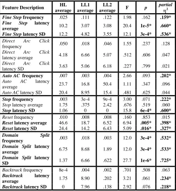
Table II. Three-way comparisons between HL, LL1, and LL2 clusters (found when k was set to 3) along each of the 21 feature dimensions
Feature Description HL average
LL1 average
LL2
average F p
partial
η2
Fine Step frequency .025 .111 .122 1.98 .162 .159*
Fine Step latency
average 10.2 3.07 3.08 20.4 1e-5* .660*
Fine Step latency SD 12.2 4.82 3.55 12.1 3e-4* .536*
Direct Arc Click
frequency .050 .018 .046 1.55 .237 .128
Direct Arc Click
latency average 4.18 6.66 5.07 .512 .606 .047
Direct Arc Click
latency SD 3.63 5.06 6.18 .227 .799 .021
Auto AC frequency .007 .003 .004 2.66 .093 .202*
Auto AC latency
average 23.7 16.8 50.4 1.11 .347 .096
Auto AC latency SD 20.4 8.95 15.4 .481 .625 .044
Stop frequency .003 3e-4 9e-4 3.00 .071 .222*
Stop latency average 1.75 .375 2.42 .676 .519 .060
Stop latency SD 1.06 0 0 15.8 6e-4* .600*
Reset frequency .010 .008 .008 .160 .853 .015
Reset latency average 46.6 18.7 6.52 6.94 .005* .398*
Reset latency SD 24.4 14.2 6.43 5.09 .016* .327*
Domain Split
frequency .003 .018 .003 12.0 3e-4* .532*
Domain Split latency
average 6.75 8.68 1.89 12.0 3e-4* .533*
Domain Split latency
SD 1.37 6.66 .622 27.7 1e-6* .725*
Backtrack frequency 8e-4 .004 .002 .701 .508 .063 Backtrack latency
average 1.75 8.90 .202 3.21 .061 .234*
Backtrack latency SD 0 7.96 .138 2.92 .076 .218*
Table III. Post-hoc pair-wise comparisons between HL, LL1, and LL2 clusters (found when k was set to 3) along each of the 21 feature dimensions
HL vs. LL1 HL vs. LL2 LL1 vs. LL2 Feature Description
pHSD d pHSD d pHSD d
Fine Step frequency .142 1.10* .078 1.48* .691 .106
Fine Step latency
average 1e-5* 1.98* 1e-5* 1.85* .818 .007
Fine Step latency SD .001* 1.68* 1e-4* 2.33* .395 .356
Direct Arc Click
frequency .216 .618 .751 .065 .147 .616
Direct Arc Click latency
average .389 .454 .667 .221 .449 .295
Direct Arc Click latency
SD .670 .254 .516 .420 .661 .126
Auto AC frequency .046* .745 .076 .666 .595 .228
Auto AC latency average .72 .476 .403 .522 .198 .471 Auto AC latency SD .386 .466 .631 .187 .491 .262
Stop frequency .031* 1.21* .081 .783 .449 .296
Stop latency average .552 .966* .692 .169 .287 .387
Stop latency SD 5e-5* 1.16* 3e-5* 1.16* .823 0
Reset frequency .562 .276 .620 .187 .744 .070
Reset latency average .031* .673 .002* 1.01* .194 .867
Reset latency SD .136 1.08* .007* 1.84* .125 .601
Domain Split frequency .003* 1.91* .820 .011 2e-4* 1.69*
Domain Split latency
average .350 .483 .019* 1.24* 1e-4* 1.79*
Domain Split latency SD 1e-4* 2.83* .488 .527 0* 2.73*
Backtrack frequency .358 .611 .721 .220 .342 .365 Backtrack latency
average .167 .745 .667 .648 .028* .934*
Backtrack latency SD .118 .867* .811 .556 .042* .851*
* Significant at pHSD<.05 or d>.8 (feature description and values in bold)
As before, here we discuss the results in Tables II and III for individual or combinations of dimensions in order to characterize the interaction behaviors of students in each cluster.
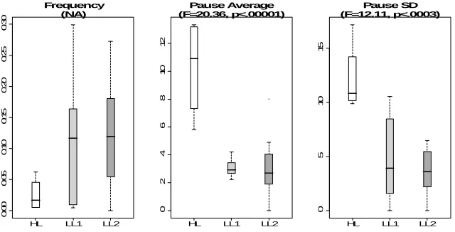
We found distinguishing Fine Step behaviors between the HL students and students in both LL clusters, similar to what we had found for the k-2 clusters. First, there was a non-significant trend of both the LL1 and LL2 students having a higher frequency of Fine Stepping than the HL students (see left box plot in Figure 5). Both the average and the
suggesting that LL students consistently pause less than HL students after a Fine Step, and that this reduced attention may have negatively affected their learning.
HL LL1 LL2
0 .00 0 .05 0. 1 0 0. 15 0 .20 0. 2 5 0. 3 0 Frequency (NA)
HL LL1 LL2
0246 8 1 0 1 2 Pause Average (F=20.36, p<.00001)
HL LL1 LL2
0 5 10 15 Pause SD (F=12.11, p<.0003)
Fig. 5. Fine Step boxplots between HL (white), LL1 (light gray), and LL2 (gray) clusters. From left to right: frequency, latency average, and latency standard deviation
The patterns of usage for the Auto AC, Stop and Reset functionalities were also similar to those we found with the k-2 clusters. That is, the HL students used the Auto AC feature more frequently than students in both LL clusters (the difference is statistically significant between the HL and LL1 clusters), suggesting that the HL students were using these features to selectively forward through the AC-3 algorithm to learn. The HL students also paused longer and more selectively after Resetting than both the LL1 and LL2 students, suggesting that the HL students may be reflecting more on each problem.
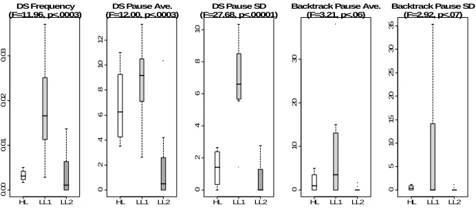
The k-3 clustering also reveals several additional patterns, not only between the HL and LL clusters, but also between the two LL clusters, indicating that k=3 was better at discriminating relevant student behaviors. For example, the k-2 clusters showed that the LL students used the Domain Split feature more frequently than the HL students, however, the k-3 clustering reveals a more complex pattern (visualized in the boxplots in Figure 6). This pattern is summarized by the following combination of findings:
• LL1 students used the Domain Split feature significantly more than the HL students.
• HL and LL2 students used the Domain Split feature comparably frequently.
• HL and LL1 students had similar pausing averages after a domain split, and paused
significantly longer than the LL2 students.
• LL1 students paused significantly more selectively (had higher standard deviation
for pause latency) than both HL and LL2 students.
Effective domain splitting is intended to require thought about efficiency in solving a CSP given different possible splits, and so the HL students’ longer pauses may have contributed to their better learning as compared to LL2 students. However, it is interesting that the LL1 students paused for just as long after Domain Splitting as the HL students, and more selectively than both the HL and LL2 students, yet still had low learning gains. The fact that LL1 cluster is also characterized by longer pauses after Backtracking may indicate that long pauses for LL1 students indicated confusion about
these applet features or the concepts of domain splitting and backtracking, rather than effective reflection. This is indeed a complex behavior that may have been difficult to identify through mere observation.
HL LL1 LL2
0. 00 0. 01 0. 02 0. 03 DS Frequency (F=11.96, p<.0003)
HL LL1 LL2
0246 8 1 0 1 2
DS Pause Ave. (F=12.00, p<.0003)
HL LL1 LL2
0
246
8
1
0
DS Pause SD (F=27.68, p<.00001)
HL LL1 LL2
01 0 2 0 3 0
Backtrack Pause Ave. (F=3.21, p<.06)
HL LL1 LL2
0 5 1 0 15 20 25 30 35
Backtrack Pause SD (F=2.92, p<.07)
Fig. 6 Domain Split and Backtrack boxplots between HL (white), LL1 (light gray), and LL2 (gray) clusters. From left to right: Domain Split frequency, Domain Split latency average, Domain Split latency standard deviation, Backtrack latency average, and Backtrack latency standard deviation.
3.3 Online Recognition and Model Evaluation for the CSP Applet
The final step in our user modeling framework (see Section 2.2) is to use the offline clusters to train classifier user models. Therefore, we built and evaluated both a two and three-class k-means classifier. These classifier user models can then take online data on a new student’s interaction with the CSP Applet (represented as a sequence of feature vectors), and classify that student into one of the offline clusters.
3.3.1 Model Evaluation for the CSP Applet (k=2)
The estimated stability cost of using the LOOCV strategy to evaluate the classifier user model trained with the k-2 clusters (two-class k-means classifier from now on) is 0.05 (averaging over the 24-folds). As discussed in Section 2.3, this is considered a very low cost, indicating that our k-2 clusters are relatively stable during the LOOCV evaluation. Therefore, a classification by the two-class k-means classifier means that a new student’s learning behaviors are similar to those of either the HL or LL clusters identified in the offline phase (Section 3.2.2).
Figure 7 shows the average accuracy of the two-class k-means classifier in predicting the correct classifications of each of our 24 students (using the LOOCV strategy) as they interact with the CSP Applet.
Fig. 7. Performance of the CSP Applet user models (k=2) over time
accuracy level. The trends in Figure 7 show that the overall accuracy of this classifier improves as more evidence is accumulated, converging to 87.5% after seeing all of the student’s actions. Initially, the classifier performs slightly worse than the baseline model, but then it starts outperforming the baseline model after seeing about 30% of the student’s actions. The accuracy of the classifier model in recognizing LL students remains relatively consistent over time, converging to approximately 90%. In contrast, the accuracy of the model in recognizing HL students begins very low, reaches relatively acceptable performance after seeing approximately 40% of the student’s actions, and eventually converges to approximately 75% after seeing all of the student’s actions (although at the very end it dips to 65% after being at 75% for over 50% of the students’ actions). It should be noted that the baseline approach would consistently misclassify HL students and thus interfere with the unconstrained nature of ELE interaction for these students. While the performance of the classifier in detecting HL students is better than the baseline, it may still cause a system based on this model to interfere with an HL student’s natural learning behavior, thus hindering student control, one of the key aspects of ELEs. The imbalance between accuracy in classifying LL and HL students is likely due to the distribution of the sample data [Weiss and Provost 2001] as the HL cluster has fewer data points than the LL cluster (4 compared to 20). This is a common phenomenon observed in classifier learning. Collecting more training data to correct for this imbalance, even if the cluster sizes are representative of the natural population distributions, may help to increase the classifier user model’s accuracy on HL students [Weiss and Provost 2001].
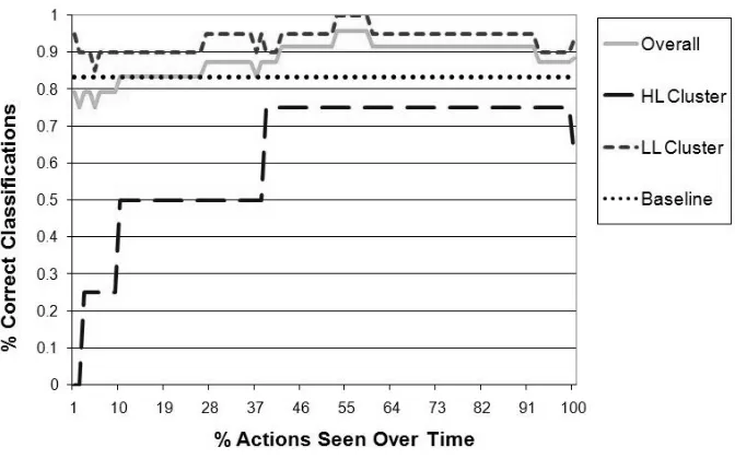
3.3.2 Model Evaluation for the CSP Applet (k=3)
The stability cost for using the LOOCV strategy to evaluate the three-class classifier user model is estimated at 0.09. The stability cost for this classifier is still low, although slightly higher than for the two-class classifier. This likely reflects the fact that the k-3 clusters are smaller than the k-2 clusters and thus less stable (i.e., removing a data point is more likely to produce different clusterings during LOOCV).
all of the actions. After seeing approximately 30% of the student actions, the classifier user model outperforms the baseline model which has a consistent, 50% (12 out of 24) accuracy rate.
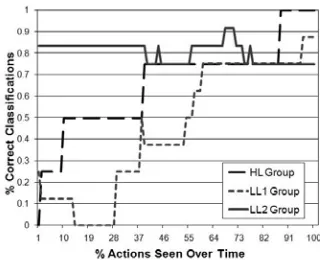
Fig. 8. Performance of the CSP Applet user models (k=3) over time
Fig. 9. Performance of the CSP Applet user models (k=3) over time for the individual clusters
Figure 9 shows the prediction accuracy trends for the individual clusters. For the HL cluster, the classification accuracy (dashed line) again begins very low, but reaches 75% after seeing about 40% of the actions, and then eventually reaches 100% after seeing all of the actions. The accuracy of the model at classifying LL1 students (dotted line), also begins low, but then reaches approximately 75% after seeing about 60% of the actions, and converges to approximately 85%. The accuracy for the LL2 students (solid line), remains relatively consistent as actions are observed, eventually reaching approximately 75%.
As with the increase in the stability cost, the lower accuracy of this classifier user model is likely an artifact of the fewer data points within each cluster. Further supporting this hypothesis is the fact that the LL2 cluster, which had 12 members, had the highest classification accuracy (80.3% averaged over time) whereas the HL and LL1 clusters, which had only 4 and 8 members respectively, had visibly lower classification accuracies (66.3% and 44.9% averaged over time, respectively). Therefore, more training data should be collected and used, particularly as the number of clusters increases, when applying our user modeling framework.
The second application we use to test our proposed user modeling framework is the Adaptive Coach for Exploration (ACE) [Bunt et al. 2001], an ELE for the domain of mathematical functions. ACE’s interface provides tools to support student-led exploration of the target domain while an adaptive Coach guided by a knowledge-based user model provides tailored suggestions on how to improve exploration.
The ACE environment is comprised of three units, each designed to present concepts pertaining to mathematical functions in a distinct manner. In this research we focus on the Plot Unit because it offers the widest range of exploratory activities of all the units by enabling students to experiment with textual as well as graphical function representations. Here, we first describe ACE’s Plot Unit and the interface actions that make up possible student interaction behaviors (Section 4.1). In Section 4.2 we present the results of applying the offline component of our framework to automatically identify clusters of students who interact similarly with ACE. In Section 4.3 we apply the online component to build a user model for ACE, and then evaluate the model.
4.1 The ACE Plot Unit
ACE’s Plot Unit interface (see main window in Figure 10) is divided into the following three components. The function exploration component (top-left panel) visually demonstrates the relationship between mathematical equations and their corresponding plots in a Cartesian coordinate plane. The Coach component (bottom-left panel) is where tailored, on-demand hints are presented to guide student exploration. And finally, the help component (right panel) contains hypertext help pages about ACE’s interface and mathematical functions.
Fig. 10. Main ACE interface window, Lesson Browser window (top right), Exploration Assistant window (bottom right), and Coach intervention window (top left)
ACE includes a knowledge-based user model of student exploration behavior that guides the Coach’s hints and interventions to improve those behaviors that are deemed to be suboptimal [Bunt and Conati 2003]. The model is a hand-constructed Dynamic Bayesian Network (DBN) that assesses the effectiveness of students’ exploration behavior based on coverage of their actions and latency. The latter is used as an estimate of a student’s active reasoning on each exploration case.
In the rest of this section, we briefly describe all of the functionalities provided by the ACE Plot Unit that form the underlying feature set on which we apply our user modeling framework to.
• Plot Move (PM). Allows the student to directly manipulate a given function by
dragging the function’s plot around the coordinate plane. The parameters of the function’s equation are automatically adjusted to reflect the transformations.
• Equation Change (EC). Allows students to edit a function’s equation (at the bottom
of the function exploration panel) and analyze the effects of the corresponding changes to the plot.
• Reset. Lets the student reset the current function to its initial parameter values (i.e.,
the function equation (see the magnifying glass icons at the bottom of the function exploration panel).
• Next Exercise (NE). Steps sequentially forward to the next exercise in ACE’s
pre-defined curriculum. This functionality is accessible by clicking on the next exercise button at the top right of the coordinate plane.
• Step Forward (SF). Performs the same functionality as the next exercise button. The
step forward arrow button is on the button toolbar at the top left of the coordinate plane.
• Step Back (SB). Steps backwards to the previous exercise in the curriculum (see
backwards arrow on the button toolbar).
• Lesson Browser (LB). Outlines ACE’s pre-defined curriculum (accessible by
clicking the scroll icon on the toolbar). The LB tool (see top right window in Figure 10) allows students to freely explore exercises within the curriculum in any order by letting students choose which exercise to examine next.
• Exploration Assistant (EA). Helps students monitor and strategically plan their
exploration within each exercise which is an important meta-cognitive activity believed to benefit learning [Gama 2004]. The EA tool (accessible by clicking on the street-sign icon on the toolbar) displays the relevant exploration cases for the current function type, and marks the cases already examined by the student. For example, the bottom right window in Figure 10 shows that the student has explored the positive intercept and negative intercept cases of a linear function, but has not yet experimented with the zero, positive or negative slope cases.
• Get Hint (GH). Requests a hint from the Coach which is displayed in the Coach
panel. Each click of the GH button (at the top of the Coach panel) displays increasingly detailed hints on what cases to explore next based on the DBM model’s current assessment of the student’s progress (see text in the Coach panel in Figure 10).
• Stay. In addition to providing on-demand hints, ACE’s Coach intervenes through a
• Move On (MO). Lets the student ignore the Coach’s advice to stay on the current
exercise and moves on to another one.
• Help. Lets the student explore the hypertext help pages available through the help
component.
• Zoom. Zooms into, or out of the graph region allowing students to inspect the plot at
different scales. Accessible through the toolbar next the function equation (see the zoom-in, ‘+’, and zoom-out, ‘-‘, magnifying glass icons at the lower left of the exploration panel in Figure 10).
4.2 Offline Identification for ACE
In this section, we describe how we applied the offline steps outlined by our user modeling framework to the ACE learning environment.
Data Collection. The data we use for the current research was obtained from a previous user study investigating how to model meta-cognitive behaviors of students using the ACE Plot Unit [Conati et al. 2005; Merten and Conati 2006]. The particular meta-cognitive behavior studied is known as self-explanation [Chi et al. 1989], the domain-independent skill of self-generating interpretations and reasoning about instructional material. This behavior has been shown to improve learning [Chi et al. 1989; Conati and VanLehn 2000; Ferguson-Hessler and Jong 1990] and so is modeled in ACE’s DBN (discussed above in Section 4.1) as one of the factors that determine the effectiveness of a student’s exploration.
The original ACE DBN user model used only latency (after plot moves or equation changes) as implicit evidence of self-explanation. However, latency alone does not assure
that the student is even attending to the material. For this reason, eye-tracking data was obtained during the user study to see whether the addition of specific eye-gaze patterns would better estimate self-explanation. The eye-gaze patterns explored were direct and indirect gaze shifts between the plot and equation areas, because, intuitively, shifting attention between the plot and equation areas is a good indication of self-explanation of the current exploration case. Figure 11 shows an example of a direct gaze shift after an equation change. The student’s gaze starts from the function equation and shifts directly
Fig. 11. Example gaze shift
A total of 36 university students participated in the user study. These students that had not taken high school calculus or college level math. Before using ACE, each student took a 15 minute pre-test on mathematical functions. Then the students interacted with ACE for as much time as needed to explore all of the exercises in each unit, with the Plot Unit providing three exercises (one constant function exercise, one linear function, and one power function). While using ACE, students were asked to follow a think-aloud protocol in which they should try to verbalize all of their thoughts. The student’s gaze was tracked by a head-mounted, Eyelink I eye-tracker developed by SR Research Ltd., Canada. Finally, the students took another 15 minute post-test that differed from the pre-test only on parameter values and question ordering.
The data from this user study was used to build a new version of the ACE user model [Conati and Merten 2007] using a supervised data-based approach with hand-labeled data. This new model used gaze information, in addition to latency between actions, to assess effectiveness of student exploration for learning. Two researchers (to assure coding reliability) labeled each student’s verbalizations after every equation change and plot move as an instance of reflection or speech not conducive to learning. These labels
was limited to direct and indirect gaze shifts only after an equation change or plot move action, although gaze shifts may also be relevant after other interface actions. For instance, after a next exercise action, a new function appears on the screen requiring attention to both the plot and equation regions in order to understand the connection between the new function equation and its plot). We will see that our framework can detect additional patterns with limited additional work.
For our current experiment we used time-stamped and logged user interactions (corresponding to all of the 13 Plot Unit interface functionalities described in Section 4.1) and synchronized eye-tracking data from ACE’s Plot Unit. From this we obtained 3783 interface actions (recorded over 673.7 minutes) along with the accompanying gaze-shift data. The pre and post-tests used in the study were devised in such a way as to evaluate relevant knowledge gained from each ACE unit separately. This allowed us to extract the test results for only the Plot Unit for the current experiment.
Preprocessing and Unsupervised Clustering. We extracted two different sets of features from the ACE study data. The first set (FeatureSet1) consisted of 39 features corresponding to the frequency of each of the 13 possible interface actions (see Section 4.1), and the average and standard deviation of the latency between each of these actions. This feature set is analogous to the one used in our first experiment (Section 3.2). We chose this feature set in order to evaluate how our modeling framework transfers across different applications using the same type of input data.
With only 36 feature vectors corresponding to the 36 study participants, the high-dimensional feature spaces of both FeatureSet1 and FeatureSet2 can result in data sparseness and may degrade the performance of clustering. Therefore, as outlined in our modeling framework in Section 2.1, we performed entropy-based feature selection [Dash and Liu 2000] on each set in order to isolate the most discriminatory features. This feature selection algorithm performs clustering on feature subsets in order to assess the quality of the features in distinguishing clusters. Therefore, by using this feature selection algorithm, we obtain both a set of relevant features, as well as the resulting clusters (the Unsupervised Clustering step of our user modeling framework, see Section 2.1) using that feature set. As for our first experiment, we used k set to 2, 3 and 4 for the k-means clustering executed during forward selection. Again, we chose these values because our data set was relatively small and so we only expected to find a few distinct clusters.
Most of the interface related features (between 34 and 37 features) were retained by feature selection on FeatureSet1. The features that were removed were all related to the standard deviations of the latency after some of the interface actions (e.g., after Lesson Browser, Exploration Assistant, Get Hint, and Stay actions).
Approximately one third of the features from FeatureSet2 (also between 33 and 37 features) were found to be relevant by feature selection. In this case, all action frequencies were deemed important for cluster formation by feature selection, except in the case of a Stay action. Also, gaze shift dimensions are only identified as important in the presence of the corresponding latency dimensions after an action. For example, indirect gaze shifts were found to be relevant in addition to the latency dimensions after an equation change, next exercise, step back, stay, and zoom action. Conversely, latency was found to be relevant independently of gaze shift features after some actions (namely after reset, step forward, Exploration Assistant, move on, and help actions). This agrees with the findings in [Conati and Merten 2007] that gaze shifts may be important mostly in discriminating between time spent self-explaining the results of an action and idle time. Interestingly, neither latency nor gaze shifts were found to be relevant after a function plot move. Given that both plot moves and equation changes are exploratory actions requiring equivalent self-explanations, this result is unintuitive especially considering that latency and gaze shifts were found to be important after equation changes. This could be an artifact of the feature selection algorithm that we use [Dash
significant differences in learning gains were found between any of the clusters. Therefore, these findings could challenge our prior beliefs about the utility of plot move exploratory actions for learning.
As discussed in our first experiment, the general rule of thumb would suggest using between 3 to 7 features for model learning given our 36 feature vectors [Jain et al. 2000]. However, because we are trying to reduce the time and effort required of application and domain experts with our user modeling framework, we decided against the time-consuming and potentially inaccurate manual analysis of the features that would have been required to reduce the dimensionality of these feature spaces further (see Section 2.1).
Table VI. Pair-wise comparisons between HL and LL clusters along each of the 36 feature dimensions
Feature Description HL average
LL
average DF t p Cohen’s d
PM frequency .024 .034 25.6 1.23 .116 .418 EC frequency .015 .019 19.8 .850 .203 .305 EC latency average 21.8 16.1 15.3 1.78 .047* .677 EC latency SD 10.4 6.08 11.5 1.56 .073 .636
EC indirect average 1.21 .440 12.6 2.57 .012* 1.02*
EC indirect SD 1.12 .556 13.0 2.24 .022* .886*
Reset frequency 0 .001 24.0 2.60 .008* .735
Reset latency SD 0 .051 24.0 1.44 .082 .406
NE frequency .005 .009 33.2 2.73 .005* .827*
NE latency average 18.7 13.2 21.3 3.01 .003* 1.07*
NE latency SD 10.3 7.44 18.8 1.64 .059 .594
NE indirect average 1.74 .625 16.0 5.79 1e-5* 2.18*
NE indirect SD 2.09 .715 13.5 5.03 1e-4* 1.97*
NE direct average 1.30 .201 10.6 3.36 .003* 1.41*
NE direct SD 1.79 .362 10.8 3.01 .006* 1.25*
SF frequency .008 .011 30.3 1.90 .034* .621
SF latency average 7.65 4.65 15.4 2.71 .008* 1.03*
SF latency SD 9.96 5.83 19.3 2.37 .014* .858*
SB frequency 0 2e-4 24.0 1.20 .122 .338 SB latency average 0 .400 24.0 1.68 .053 .475
SB indirect average 0 .040 24.0 1.00 .164 .283
LB frequency 0 6e-4 24.0 1.87 .037* .528
EA frequency 1e-4 .001 27.6 2.22 .018* .640
EA latency average 5.27 5.65 16.7 .072 .472 .027 GH frequency 3e-4 4e-4 34.0 .311 .312 .155 Stay latency average 6.55 2.54 14.5 2.01 .032* .775 Stay indirect average .152 .100 22.5 .389 .350 .136
MO frequency .003 .005 32.1 2.31 .014* .744
MO latency average 2.23 232 24.0 1.00 .163 .283 MO latency SD 2.76 400 24.0 1.00 .163 .283 Help frequency .002 .001 14.3 .745 .234 .288
Help latency
average 2.45 7.28 33.1 1.94 .030* .587
Zoom frequency 4e-4 .021 24.1 2.62 .008* .741
Zoom latency
average .374 1.98 29.9 2.92 .009* .961*
Zoom latency SD .700 2.70 22.6 2.24 .017* .785
Zoom direct SD 0 .101 24.0 2.41 .012* .683
* Significant at p<.05 or d>.8 (feature description and values in bold)
with k set to 2 on FeatureSet2 (k-2 clusters from now on). In this case, one cluster (of 11 students) had higher learning gains (average=2.91 points, SD=3.11) than the other cluster (25 students, average=1.20 points, SD=2.87). Therefore, in the rest of this section, we proceed to characterize only these two clusters in terms of the interaction behaviors they represent (i.e., by doing a pair-wise analysis of the differences between the two clusters along each of the 36 feature dimensions remaining after feature selection in this case). Hereafter, we refer to the cluster with high and low average learning gains as the ‘HL’ and ‘LL’ clusters, respectively. Table VI presents the results of the pair-wise analysis between the HL and LL clusters. Significant values and the corresponding feature dimensions are highlighted in bold.
Some of our findings are consistent with results in [Conati and Merten, To Appear], as we were hoping. First, there were no statistically significant differences in the frequency of plot move or equation changes between the HL and LL clusters (see ‘PM frequency’ and ‘EC frequency’ entries in Table VI), consistent with finding in [Conati and Merten, To Appear] that sheer number of exploratory actions is not a good predictor of learning in this environment. Second, after an equation change, the LL students would pause for a significantly shorter duration than the HL students on average (see ‘EC latency average’ in Table VI). In [Conati and Merten, To Appear], the authors determined 16 seconds to be an optimal threshold between occurrences of effective reflection on exploration cases and other verbalizations not conducive to learning. Consistent with this result, the second boxplot in Figure 12 shows that the average latency by the students in the HL cluster were mostly above this threshold, whereas with the LL cluster the latency averages were centered about the threshold.
HL LL 0. 00 0. 01 0. 02 0. 03 NA HL LL 0 5 10 15 20 25 30
p < .04
HL LL 0 5 10 15 2 0 25
p < .07
HL LL 0. 0 0 .5 1. 0 1 .5 2 .0 2 .5
p < .01
HL LL 0. 0 0 .5 1. 0 1 .5 2. 0
p < .02
Fig. 12. Equation Change boxplots between HL (gray) and LL (white) clusters. From left to right: frequency, latency average, latency standard deviation, indirect average, and indirect standard
Because with clustering we are able to incorporate all interface actions and associated gaze data simply by including them in the multi-dimensional feature vectors, we also found patterns additional to the ones found in [Conati and Merten, To Appear]. For example, the students in the HL cluster were more varied in how often they would indirectly gaze shift after an equation change (see the last boxplot in Figure 12). This selective behavior suggests that students need not reflect on the results of every exploratory action in order to learn well so long as they do not consistently refrain from reflection. In addition, the LL students paused less and made significantly fewer indirect gaze shifts after an equation change than the HL students (see the second and fourth boxplots in Figure 12). These results are consistent with less reflection by the LL students compared to the HL students and may account for some of the difference in learning gains. We found similar differences between the two clusters when a new function appeared on the screen after a next exercise action (see NE latency and gaze entries in Table VI).
When the Coach suggested that a student spend more time exploring the current exercise, LL students chose to ignore the suggestion and move on to another exercise significantly more frequently than HL students (see ‘MO frequency’ in Table VI). The Coach’s suggestions are intended to promote effective learning [Bunt and Conati 2003] and so it is reasonable that ignoring them would adversely affect students. Furthermore, when Stay actions occurred, HL students paused for significantly longer than LL students (see ‘Stay latency average’ in Table VI), suggesting that the HL students followed the Coach’s advice more carefully by spending additional time pondering over the current exercise before taking additional actions.
While the above patterns are quite intuitive, our approach was also able to identify additional patterns that do not have an obvious relation to learning. For example, the LL students advanced sequentially through the curriculum using the next exercise and step forward buttons significantly more frequently than the HL group (see ‘NE frequency’ and
exercise, step forward, step back, Lesson Browser, move on and stay) it may have been
difficult to observe, even by application experts.
Similarly, there were unintuitive differences in the use of the zooming features between the two clusters (see ‘Zoom’ features in Table VI). The LL students zoomed into or out of the plot region significantly more frequently than the HL students. The HL group students paused for a consistently shorter duration after zooming than the LL students on average. Although zooming may not have clear pedagogical benefits, this behavior may suggest confusion on the part of the LL students resulting in the need for more detailed inspection of the plot. LL students also paused for significantly longer after navigating to a help page then HL students (see ‘Help latency average’ in Table VI). This is also unintuitive as the help pages are intended to instruct students about how to use ACE or about relevant domain concepts and therefore would be expected to help students learn. However, considering that LL students showed low learning gains, this behavior could also be interpreted as indicating confusion.
Also detected were patterns that may reveal the inadequacy of some of ACE’s interface tools. First, there were no differences between the groups in their use of the get hint feature. And in fact, very few students in either group used this feature. This could suggest that students prefer to explore independently, or that they have little confidence in the Coach’s hints, or that they were simply not aware of this feature. This implies that further investigation is necessary to evaluate the benefits of the Coach’s get hint feature. Also, the LL students used the Exploration Assistant tool significantly more frequently than the HL students (see ‘EA frequency’ in Table VI), but still had lower learning gains. This suggests that the Exploration Assistant had little impact on overall learning contrary to its intended purpose of helping students better plan their exploration.
4.3 Online Recognition and Model Evaluation for ACE
As in our first experiment (Section 3), and as dictated by our user modeling framework (see Section 2.2), we can use the clusters found in the offline phase (described in Section 4.2) directly to train a k-means-based online classifier user model. We constructed such a model to recognize students belonging to either the HL or LL clusters found by k-means clustering (with k=2) and characterized in the previous section.
(see Section 2.3) before we draw conclusions about the predictive accuracy of the user model
The estimated stability cost for the k-means classifier user model constructed in this experiment was 0.062 after averaging the costs calculated over the 36 folds of the LOOCV evaluation (recall that 0 is considered perfect stability and 1 is considered maximum instability [Lange et al. 2003]). This means that the characteristic behaviors of the two clusters identified in the offline phase are reasonably preserved during our LOOCV evaluation.
Figure 13 shows the average percentage of correct predictions as a function of the percentage of actions seen by the k-means online classifier model (solid line). The accuracy of the model (averaged over all of the students) converges to 97.2% after seeing all of the students’ actions. For comparison, the figure also shows the performance of a likely class baseline model that always classifies new student actions into the most-likely (or largest) class (i.e., the LL cluster of 25 students in this case), and therefore the baseline model accuracy is shown by the dashed line straight across the figure at the 69.4% (25/36) accuracy level. The figure shows that the k-means classifier model outperforms the baseline model after seeing only 2% of the student actions. The figure also shows the k-means classifier model’s performance over both the HL and LL clusters (dashed and dotted lines, respectively). The accuracy for the LL group remains relatively stable over time, whereas the performance for the HL group is initially poor but increases to over 80% after seeing about 45% of the actions.
As in our first experiment, the imbalance in accuracy between the classification of HL and LL learners is likely the result of the smaller sample of data from the HL cluster compared to the LL cluster.
5. COMPARISON OF EXPERIMENTS
One of the goals of this work is to show that our proposed modeling framework works on different domains and data sets, therefore, in this section, we compare and contrast the experimental results we obtained by applying the framework to two different learning environments, the AIspace CSP Applet and ACE and using two different types of input data. Both of these environments provide various interaction mechanisms that allow for uninhibited student exploration of the target domain, and may benefit from the inclusion of adaptive guidance that can help students gain the most from their exploration process.
5.1 Comparison of Results from the Offline Identification Phase
In both of our experiments, cluster analysis demonstrated that unsupervised clustering in the framework’s offline component was able to identify distinct clusters of students (i.e., clusters of students showing differences in learning outcomes from pre to post-tests). In addition, the analysis revealed several characteristic learning behaviors of the distinct clusters. Some of these characteristic behaviors were intuitive and thus reasonably explained either the effective or ineffective learning outcomes. However, as expected, some of the behaviors did not have obvious learning implications, requiring consideration of combinations of dimensions (as k-means does to determine its clusters), or knowledge of the student learning outcomes to be explained. These latter behaviors would have been difficult to recognize and label by hand, even by application experts.
There are, however, two discrepancies in our results that need to be examined: 1. Clustering found distinct clusters when k was set to 2 and 3 in our first experiment
with the CSP applet, but only found distinct clusters for k set to 2 in our second experiment with ACE.
2. Clustering was able to find clusters within the CSP applet data using interface actions alone, whereas it only found distinct clusters for ACE when we used a dataset that included both interface actions and eye-tracking data.
Applet interface includes several mechanisms that allow the student to visualize and reflect on the workings of the AI algorithm on a CSP, whereas ACE only provides two such mechanisms per equation type: plot moves and equation changes. Therefore, the CSP Applet interface supports a larger variety of interaction behaviors per problem than the ACE’s interface, which may explain why we could only identify two distinct clusters for the latter. That is, considering the variety of possible interaction behaviors with the CSP Applet, interface actions alone may be better able to capture student learning and reflection during exploration than interface actions alone in ACE. This hypothesis is consistent with the results in [Conati and Merten, To Appear] showing that gaze patterns, together with action latency, predict student reflection and learning in ACE better than sheer number of actions or action latency alone. Additional data may be necessary [Jain et al. 2000] to detect distinct clusters of learners with ACE using only this first feature set.
5.2 Comparison of Results from the Online Recognition Phase
To facilitate the comparison of the classifier student models used in the on-line recognition phase for the CSP Applet and ACE, Table VIII reports accuracy in classifying HL and LL students, averaged over time. The table also shows the accuracies of the corresponding baseline models that used most-likely-class classification strategies. In all cases, the k-means based user models outperformed the corresponding baseline models on predicting the correct class for new student behaviors.
Table VIII. Summary of classification accuracies averaged over time
CSP (k=2)
CSP
(k=3) ACE
Overall Accuracy 88.3% 66.2% 86.3%
Accuracy on LL students 93.5% 66.1% 94.2% Accuracy on HL students 62.4% 63.3% 68.3%
Baseline Accuracy 83.3% 50.0% 69.4%