Including traffic jam avoidance in an
agent‑based network model
Christian Hofer
*, Georg Jäger and Manfred Füllsack
Background
Simulating and understanding (urban) traffic is an important challenge related to many different scientific fields like urban planning, transportation planning, and sustainability. The goals of traffic simulations can be manifold and include gaining insight into traffic-related noise pollution [1], finding ways to reduce emissions [2], or analyzing the effects of policies [3]. To reach these goals, many different approaches to traffic simulations exist (see, for example, [4] for a detailed overview).
In general, traffic models can be divided into two categories, namely bottom–up and top–down approaches. Bottom–up approaches start from individual vehicles and simu-late their behavior to find aggregated macro-scale results. Most bottom–up approaches
Abstract
Background: Understanding traffic is an important challenge in different scientific fields. While there are many approaches to constructing traffic models, most of them rely on origin–destination data and have difficulties when phenomena should be investigated that have an effect on the origin–destination matrix.
Methods: A macroscopic traffic model is introduced that is novel in the sense that no origin–destination data are required as an input. This information is generated from mobility behavior data using a hybrid approach between agent-based modeling to find the origin and destination points of each vehicle and network techniques to find efficiently the routes most likely used to connect those points. The simulated road uti-lization and resulting congestion is compared to traffic data to quantitatively evaluate the results. Traffic jam avoidance behavior is included in the model in several variants, which are then all evaluated quantitatively.
Results: The described model is applied to the City of Graz, a typical European city with about 320,000 inhabitants. Calculated results correspond well with reality.
Conclusions: The introduced traffic model, which uses mobility data instead of ori-gin–destination data as input, was successfully applied and offers unique advantages compared to traditional models: Mobility behavior data are valid for different systems, while origin–destination data are very specific to the region in question and more diffi-cult to obtain. In addition, different scenarios (increased population, more use of public transport, etc.) can be evaluated and compared quickly.
Keywords: Agent-based model, Spatial networks, Traffic simulation, Origin– destination data, Congestion analysis
Open Access
© The Author(s) 2018. This article is distributed under the terms of the Creative Commons Attribution 4.0 International License (http://creat iveco mmons .org/licen ses/by/4.0/), which permits unrestricted use, distribution, and reproduction in any medium, provided you give appropriate credit to the original author(s) and the source, provide a link to the Creative Commons license, and indicate if changes were made.
RESEARCH
are micro-scale agent-based car-following models; prominent examples are the open source projects MatSIM [5] and SUMO [6] or the commercially available software VIS-SIM [7]. The downside of such detailed bottom–up approaches is that they need a lot of input data, in some cases complete origin–destination matrices, i.e., the complete infor-mation what vehicle drives from which starting point to which destination. In addition, their computation time is relatively high, so that calculation in real time may only be possible for small systems. A completely different approach is used for top–down mod-els. Their starting point is the macro-scale, i.e., statistical information about traffic flow or other macroscopic properties. Such statistical models can, for example, be used to calculate emissions [8] very efficiently.
Both bottom–up and top–down approaches can utilize networks or more specifically spatial networks [9], in the simplest case to represent the road network, but also more sophisticated network methods can be incorporated in a traffic model [10], to focus on the network itself, rather than the vehicles using the road network, which can signifi-cantly speed up computation time [11].
In this study, we use a hybrid approach [12], combining features of both bottom–up and top–down methods. One of the biggest challenges in traffic simulation is to obtain realistic origin–destination data. This can be done by combining traffic count with sur-vey data [13] or by utilizing information from a mobile-phone network [14]. In this study, we use survey data about the mobility behavior of citizens to generate realistic ori-gin–destination data within the model. This approach has many advantages; for exam-ple, it is straightforward to evaluate various scenarios, like a certain change in mobility behavior (more use of public transport, an increased popularity of online shopping, and telecommuting) as well as juridical changes, changes in the infrastructure, or techno-logical changes, all within the same framework. This makes the model especially power-ful and versatile for the evaluation of the impact of various policies. The starting point of this study is the idea presented in [15], but goes beyond this by investigating traffic jam avoidance behavior and developing a technique to quantitatively evaluate the validity of the road usage data produced in a network-based traffic model. As a case study for eval-uation we choose the City of Graz, an Austrian city with about 320,000 people, because it is a typical European city of this size.
This paper is organized as follows: "Methods" section describes the model develop-ment and gives details on the process used for evaluation. "Results" section presents the obtained results, primarily focusing on the question whether realistic road usage data could be obtained. "Discussion" section concludes with limitations and possible expan-sions of the presented model.
Methods
obtained in an agent-based process. Traffic jam avoidance effects are then included via an iterative method. Finally, obtained results are evaluated quantitatively.
Generating a road network representation
To obtain a network representation of the investigated area, we use map data obtained
from OpenStreetMap [17]. Such data are available for most of the world in varying
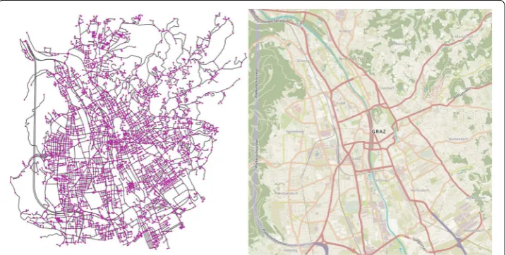
degrees of detail and can include not only the geographical position of each road sec-tion, but also additional relevant data, like the width of the road, the number of lanes, the maximally allowed speed, whether it is a one-way street or not and other important features. To convert these data to a network, the library OSMnx [18] is used. This library uses the OpenStreetMap data, identifies relevant points in each road (intersections, forks, dead ends, ... ), and uses them as nodes for the network. The edges of the network are the road sections connecting the nodes, including relevant information about the road as edge variables. That way, an accurate network representation of the investigated infrastructure can be obtained in an automated way, shown for the City of Graz in Fig. 1.
Additional information that could be interesting, like, for example, population density or the position of relevant business or industrial hubs can be included via an additional OpenStreetMap import. In this example, we matched each node to a district of Graz, to utilize population density information with district resolution. Including other informa-tion was not necessary, mainly because the investigated city features a simple structure, where important business and industrial hubs coincide with high population density, yet inclusion of such data would be straightforward.
Calculating fastest paths
During the simulation, it is often necessary to find the shortest path between two nodes, or more precisely, to find out which nodes are within a certain distance of a starting point, using shortest paths. Note that all shortest paths are weighted with the average
travel time of the involved edges, so the shortest paths are in a sense fastest paths. This operation is computationally quite time consuming, so to optimize efficiency, it is per-formed before the simulation itself. Specifically, we calculate the length of the shortest paths between each and every node and save the information which nodes are up to x meters away from the original node, with x binned in 100 m bins. This makes finding valid target nodes (a process explained in "Calculating road usage" section) much faster. To further increase the speed of the simulation, it would be possible to use a graphics card for shortest path calculations or to store not only the distances, but the complete paths, if enough memory is available.
Obtaining mobility behavior from survey data
The distinctive feature of the presented model is that no origin–destination data are required as input data. This information is generated from mobility behavior, gathered in the survey “Österreich Unterwegs 2013/2014” [16]. In this survey, 18,000 respond-ents from Austria reported their mobility behavior on 2 separate days, leading to 36,000 days of mobility data, randomly distributed over the year. Each day contains all the trips which a respondent performed (length of the trip, used transportation method, details of the car, if a car was used, and reason for the trip) as well as information about the respondent.
In principle, it would be possible to use the full set of data, but the predictive power of the model can be improved by restricting the data to data sets that were obtained in areas that are similar to the investigated system (i.e., small town, big cities,...). In this study, where the City of Graz is investigated, we restricted the mobility data to data obtained in Graz, which truncated the data set to 1800 days of mobility data.
These data are used to generate a pool of mobility behaviors, i.e., sets of daily driv-ing behavior patterns. Each day of mobility behavior can contain several trips and each trip is primarily classified by its length and the used method of transportation. How-ever, these data do not contain any specific origin or destination points, so, to calculate actual traffic data, we use a multi-agent approach, presented in "Calculating road usage" section.
Calculating road usage
node are determined, a calculation of the fastest path between them is performed. This path is then used by the agent, using the correct mode of transportation, as given in the trip data. The destination node then becomes the origin node for the next trip and the process is repeated until all agents performed all their trips.
For certain cities, where commuting from regions outside the simulation area is rel-evant, it is intuitive to include such trips. Therefore, we also include agents with a start-ing point outside the city. Statistical data about which region they come from and which entry node is thus most likely used to enter the city were obtained from [19]. These com-muting agents are especially important when investigating traffic jams, since they are mostly active during times of peak activity.
Including traffic jam
To investigate the occurrence of traffic jams, we first need to calculate the daily traffic capacity for each section of road. For this, we need information about the width of the road, the number of lanes and if this section of road is a one-way street or not, which is already included in the road network. Using these data, we can calculate the daily traffic capacity C for each section of road [20]. To obtain the hourly traffic capacity Ch, special conversion factors are used [21] and Ch is then calculated from
where Leff is the effective number of lanes. The starting point of finding Leff is the actual number of lanes, if it is known. If this number is unknown, because this information is missing in the imported map data, approximate values are derived from the width of the road: Leff= 2.6 for roads wider than 7.5 m, Leff= 2.0 for roads between 7.5 and 5.5 m, and Leff= 0.8 for roads narrower than 5.5 m [21]. This number is then halved for roads that are not used as one-way streets, since then only half of the lanes can be used in one direction, to find the final value for Leff and thus C
h. To find out if the traffic flows freely or a traffic jam occurs, we compare the hourly number of vehicles Vh with the hourly traffic capacity Ch:
The obtained load quotient a is then used to differentiate between different stages of congestion. a smaller than 0.75 signifies free-flowing traffic, a between 0.75 and 0.9 is a sign of constrained traffic flow and a larger than 0.9 can be interpreted as stop-and-go traffic [21]. That way, a first approximation to the traffic conditions of each section of road can be obtained. This approximation can be further refined by including traffic jam avoidance in an iterative process. After calculating the approximated traffic conditions, agents react to the resulting congestion, by avoiding routes that are heavily congested and using alternative routes. In the model, this is done by keeping the origin–destina-tion pairs constant (i.e., origin nodes and destinaorigin–destina-tion nodes of agents do not change) and recalculating the shortest paths, now including delays caused by congestion. This leads to new traffic conditions and in turn a new congestion status for every section of road in (1) Ch=Leff750 cars
hour
(2) a= Vh
the system. This updated congestion information can again be used to refine the traffic data by recalculating shortest paths.
However, not all drivers change their route due to congestion effects. De Palma et al. [22] found that only 30% of commuters use different routes to avoid traffic jams. Thus, the starting point of our investigation is the situation that 30% of all agents are avoiding traffic jams, while the other 70% remain on their original paths at all times. In addition to this scenario, we explore more of this parameter space, by varying the percentage of congestion avoiding agents between 0 and 50%. By comparing the simulated results to congestion forecasts based on real traffic data, we find out which parameter leads to the most realistic result.
Quantitative evaluation using congestion data
To evaluate the obtained congestion data quantitatively, statistical travel times that include congestion effects are extracted for every road segment from the Google Maps Distance Matrix API [23]. The travel times of a typical midweek morning (between 7 and 8 a.m.) with no nearby public holidays are used as peak travel times, while travel times with negligible traffic (early hours after midnight) are used as reference points. From this, the relative time lost for each section of road is calculated by the following:
with the travel time with negligible traffic F and the peak travel time T. This value is then compared to the simulated results. Because the simulation yields information about the load factor a of each section of road and the resulting free-flowing or stop-and-go traffic, this value must be translated to relative time lost, to be comparable to the real world data. The simplest way to make these two related properties comparable is to use normalization, so that both values are between 0 and 1. In that way, the deviation D is calculated as follows:
with the maximal load factor amax and the maximal time lost tmax . To gain a single scalar that scores the accuracy of the simulated values, differences are calculated, and then, the values for each section of road are weighted with the corresponding travel time and summed up. This leads to the average deviation Davg of the simulation results:
with i running over all edges of the network, and Li the lengths of all sections of roads. Using this equation, it is, for example, possible to compare the validity of different parameters for including traffic avoidance strategies.
(3) t= T −F
F ,
(4) D= a
amax − t
tmax,
(5) Davg=
iabs(Di)Li
iLi
Results
Overall road usage
The main results of each simulation run are the origin–destination data itself (which could be used as an input for a microscopic car-following model), the trajectories of all cars, and overall road usage and resulting congestion.
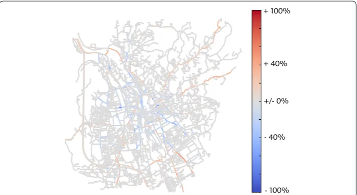
For every hour of the simulated day, the congestion is calculated as described in "Including traffic jam" section. Since the road segments are not congested most of the day and therefore not suitable for evaluation, we use the morning rush-hour between 7 and 8 a.m. for evaluation. The congestion after a first approximation of traffic with-out traffic jam avoidance is compared with congestion visualization from a weekday at
the same time from Google Maps in Fig. 2. It shows the simulated congestion without
including effects of traffic jam avoidance (left panel) compared to the actual conges-tion (right panel). The simulated congesconges-tion values are calculated from the load factor a, given in Eq. (2), during rush-hour. The right panel shows data extracted from Google Traffic, i.e., the amount of congestion during peak activity. Both values are in good agreement; most main travel routes are accurately depicted. This is not trivial, since no origin–destination data were used as an input for the model.
However, on closer inspection, there are some discrepancies between the simulated traffic data and the real traffic data. Mainly, the big roads are used extensively, so that a large amount of congestion occurs, while smaller, parallel roads are used only infre-quently. The reason for this is that traffic jam avoidance is not included yet. Accounting for this effect significantly improves the results, as can be seen in "Quantitative evalua-tion and traffic jam avoidance" section.
Quantitative evaluation and traffic jam avoidance
Including traffic jam avoidance strategies in an iterative process detailed in "Including traffic jam" section could make the obtained traffic data more realistic. However, a priori not all parameters of this technique are known. Namely, the number of iterations needed until convergence is reached is unknown, as well as the actual percentage of drivers who change their route to avoid traffic jam. To fine-tune these parameters, the method pre-sented in "Quantitative evaluation using congestion data" section is used for the evalu-ation. Using this precise feedback, how well the simulation matches the reality, we can determine the unknown parameters.
The results of the quantitative evaluation of the model are presented in Fig. 3. Shown is the relative error of congestion for each section of road for a simulation run without any traffic jam avoidance. Summing over all edges and weighting with the length of the section of road [see Eq. (5)] lead to an average deviation of 0.0301. While some sections of road are described very well, others show too much congestion, compared to reality, while others show too little.
This result can be improved by the process detailed in “Including traffic jam” section. Literature suggests that 30% of commuters change their routes to avoid traffic; neverthe-less, we scanned a bigger range of parameters, since especially in a city traffic avoidance behavior is not known precisely. In addition, we investigate the effect of several itera-tions on the validity of the simulation. This analysis is shown in Fig. 4.
It is clearly visible that traffic avoidance chances of more than 10% cannot lead to an improvement. The best match between simulated and real data is achieved for a traffic avoidance chance of 10% after one iterative step. Note, that using a 5% traffic avoidance chance also iterations 1, 3, and 5 are in relatively good agreement, while even numbered iterations perform worse in general. The reason for this effect is the iterative nature of the traffic jam avoidance. The initial guess (0) features no traffic jam avoidance. In
+ 100%
- 100% +/- 0% + 40%
- 40%
iteration 1, the agents avoid the heavily congested roads, making them less congested, corresponding to a more realistic picture. In iteration 2, some of the agents change back to the previously heavily congested roads, since they were less congested in iteration 1. This process repeats itself, so that the odd numbered iterations always produce more realistic results.
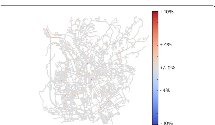
To visualize the positive effect of considering traffic jam avoidance, we calculate the
difference in D between a simulation run without traffic jam avoidance and one with
traffic jam avoidance (10%, first iteration). This difference is shown in Fig. 5. Although the change is relatively small, it reduces overall deviation to 0.0298, since most changes increase traffic in the inner city, which was one of the main errors (see Fig. 3).
Fig. 4 Deviation between simulated and real data with respect to traffic avoidance and number of iterations. The average deviation Davg for all simulation runs is compared to the reference congestion data from Google
Maps
+ 10%
- 10% +/- 0% + 4%
- 4%
Fig. 5 Difference in deviation due to traffic jam avoidance. Difference between one simulation run without traffic jam avoidance and the simulation run with the lowest Davg (10% traffic avoidance, first iteration). The
Discussion
It was possible to show that the presented model can quite accurately predict the road utilization of a given system without the need for origin–destination data. Precise knowledge about the mobility behavior is enough to gain satisfying results on which roads are used how often during which hour of the day. The main error is that traffic on the main roads leading into the city is overestimated, while inner city traffic is slightly underestimated. This effect has to do with the fact that agents always choose the fastest path, using the allowed speed limit to approximate travel time, while, in reality, heav-ily congested roads may have decreased effective speed and are, therefore, avoided by drivers. The error can be combated by including traffic jam avoidance strategies into the agents behavior.
Results showed that the best way to include traffic jam avoidance is to assume that 10% of the drivers change their route to evade congested roads. This is a lower percentage than is reported in [22]. The reason for this is that we investigated the road network of a city and that traffic jam avoidance behavior is different in an urban environment. Here, there are very few alternative paths, and even if alternative paths exist, during rush-hour, they are congested in a similar way. In addition, people as well as roads are adapted to congestion on main urban roads, so only very few drivers deviate from the prominent direct routes. One limitation of the presented model is the temporal resolution. Time is discretized in steps of 1 h. A finer discretization of time is not straightforward for the following reasons. The main advantage of the proposed model is its fast computa-tion time, compared to the tradicomputa-tional car-following models. This only works, because the actual movement of all cars is simplified drastically. Actual speed and driving time are only known on averages, but there is no information about the speed, and, there-fore, the current position of each car, only the exact paths are known. This simplifica-tion works quite well, as long as the assumpsimplifica-tion holds, that most of the cars are able to finish their routes within one unit of discrete time, i.e., here 1 h. This is reasonable in an urban environment. However, reducing the time steps to minutes would lead to the breakdown of this assumption. Additional information about the position of each vehi-cle at each minute needs to be calculated, which is much more time-consuming than the currently needed information about the path of each vehicle at each hour. Furthermore, road capacities are usually only defined in cars per day or cars per hour and it is gener-ally advised against using road capacities for shorter time periods, since they may be inaccurate [21].
Shown here is the application of the presented model to the City of Graz, however, application to a different urban system would also be possible. Map data are available from OpenStreetMap for most regions in great detail and can be imported in the same way as presented in "Generating a road network representation" section. Mobility data were collected in Austria [16], but it is reasonable to assume that mobility behavior depends more on certain specifics of a city, rather than the country the city is in, so using Austrian mobility data of a city with similar properties and structure may yield reason-able results. Alternatively, mobility behavior data from a different source, giving details about the investigated city, could be used to further improve the descriptive power of the model. That way, the presented framework could theoretically be used to simulate an arbitrary road network in the same way as was done here for the City of Graz.
Accurately depicting the correct road usage of a given system without relying on actual origin–destination data is the basis of future investigations. Now that we were able to show that the presented model produces satisfying results with quantitative evaluation, the next step is to use this model to make predictions about various scenarios. We can make significant manipulations on the road network, or change the number of agents to account for future population development. In addition, different mobility behavior can be used to evaluate various scenarios. Since we have specific information about the rea-son for each trip, we can implement societal changes, like an increase in telecommuting, unemployment, or online shopping. A rudimentary analysis using an early version of the
presented approach was performed in [24] and focused on emission, which are
espe-cially relevant in urban systems [25, 26]. Yet, that study lacked quantitative evaluation on a local scale and it used a simplified path finding algorithm, which completely neglects traffic jam avoidance behavior. Using the methods presented here, the analysis could be improved significantly, increasing the predictive power of the used model. Especially, for changes that affect inner city traffic and commuting behavior, an accurate depiction of congestion and congestion avoidance is paramount and including these effects in the way presented here would be a valuable expansion, making the results more realistic and accurate.
Authors’ contributions
CH and GJ developed the model and analyzed the results. All authors contributed to editing the final manuscript. All authors read and approved the final manuscript.
Acknowledgements
The authors would like to thank the University of Graz for the financial support regarding the publication fees.
Competing interests
The authors declare that they have no competing interests.
Availability of data and materials All relevant data are within the paper.
Ethics approval and consent to participate Not applicable.
Funding
The University of Graz offered financial support for the publication fees of this paper.
Publisher’s Note
Received: 16 February 2018 Accepted: 2 May 2018
References
1. Steele C. A critical review of some traffic noise prediction models. Appl Acoust. 2001;62(3):271–87.
2. Wang H, Fu L. Developing a high-resolution vehicular emission inventory by integrating an emission model and a traffic model: part 1—modeling fuel consumption and emissions based on speed and vehicle-specific power. J Air Waste Manag Assoc. 2010;60(12):1463–70.
3. Grote M, Williams I, Preston J, Kemp S. Including congestion effects in urban road traffic CO2 emissions modelling: do Local Government Authorities have the right options? Transp Res Part D Transp Environ. 2016;43:95–106. 4. Kotusevski G, Hawick K. A review of traffic simulation software. Res Lett Inf Math Sci. 2009;13:35–54.
5. Balmer M, Rieser M, Meister K, Charypar D, Lefebvre N, Nagel K. MATSim-T: architecture and simulation times. In: Bazzan A, Klügl F, editors. Multi-agent systems for traffic and transportation engineering. Hershey: IGI Global; 2009. p. 57–78.
6. Krajzewicz D, Hertkorn G, Rössel C, Wagner P. SUMO (Simulation of Urban MObility)-an open-source traffic simula-tion. In: Proceedings of the 4th middle east symposium on simulation and modelling (MESM20002). 2002. p. 183–7. 7. Vissim P. 5.10 User manual. Karlsruhe: PTV Planung Transport Verkehr AG; 2008.
8. Cappiello A, Chabini I, Nam EK, Lue A, Zeid MA. A statistical model of vehicle emissions and fuel consumption. In: Intelligent transportation systems, 2002. Proceedings. The IEEE 5th international conference on. IEEE. 2002. p. 801–9. 9. Barthélemy M. Spatial networks. Phys Rep. 2011;499(1–3):1–101.
10. Helbing D, Armbruster D, Mikhailov AS, Lefeber E. Information and material flows in complex networks. Phys A Stat Mech Appl. 2006;363(1):11–6.
11. Nagurney A, Dong J. A multiclass, multicriteria traffic network equilibrium model with elastic demand. Transp Res Part B Methodol. 2002;36(5):445–69.
12. Cetin N, Burri A, Nagel K. A large-scale agent-based traffic microsimulation based on queue model. In: Proceedings of swiss transport research conference (STRC), monte verita, CH. Citeseer. 2003.
13. Cascetta E. Estimation of trip matrices from traffic counts and survey data: a generalized least squares estimator. Transp Res Part B Methodol. 1984;18(4):289–99.
14. Caceres N, Wideberg J, Benitez F. Deriving origin–destination data from a mobile phone network. IET Intell Transp Syst. 2007;1(1):15–26.
15. Hofer C, Jäger G, Füllsack M. Generating realistic road usage information and origin–destination data for traffic simulations: augmenting agent-based models with network techniques. In: Cherifi C, Cherifi H, Karsai M, Musolesi M, editors. Complex networks & their applications VI. Complex networks 2017. Springer; 2018. p. 1223–1233. https :// doi.org/10.1007/978-3-319-72150 -7_99.
16. Tomschy R, Herry M, Sammer G, Klementschitz R, Riegler S, Follmer R, Gruschwitz D, Josef F, Gensasz S, Kirnbauer R, et al. österreich unterwegs 2013/2014: Ergebnisbericht zur österreichweiten Mobilitätserhebung Österreich unterwegs 2013/2014. im Auftrag von: Bundesministerium für Verkehr, Innovation und Technologie, Autobahnen und SchnellstrassenFinanzierungs Aktiengesellschaft, Österreichische Bundesbahnen Infrastruktur AG, Amt der Burgenländischen Landesregierung, Amt der Niederösterreichischen Landesregierung, Amt der Steiermärkischen Landesregierung und Amt der Tiroler Landesregierung. Herausgeber: Bundesministerium für Verkehr, Innovation und Technologie, Wien. Tuia D, de Eicker MO, Zah R. 2016.
17. Open Street Map: OpenStreetMap. Retrieved 18 June 2017.
18. Boeing G. OSMnx: new methods for acquiring, constructing, analyzing, and visualizing complex street networks. Comput Environ Urban Syst. 2017;65:126–39.
19. Statistik Austria: Registerzählung 2011. Statistik Austria Pendlerstatistik. 2011.
20. FGSV. Richtlinien Für die Anlage Von Straßen (RAS) Teil: Querschnitte (RAS-Q). Köln: FGSV-Verlag; 2006. 21. Höfler F. Verkehrswesen-Praxis Band 1: Verkehrsplanung. Berlin: Bauwerk Verlag GmbH; 2004.
22. De Palma A, Rochat D. Understanding individual travel decisions: results from a commuters survey in Geneva. Trans-portation. 1999;26(3):263–81.
23. Google Maps Distance Matrix API. 2015. https ://devel opers .googl e.com/maps/docum entat ion/dista nce-matri x/. Accessed 15 Feb 2018.
24. Hofer C, Jäger G, Füllsack M. Large scale simulation of CO2 emissions caused by urban car traffic: an agent-based network approach. J Clean Prod. 2018;183:1–10. https ://doi.org/10.1016/j.jclep ro.2018.02.113.
25. Fenger J. Urban air quality. Atmos Environ. 1999;33(29):4877–900. https ://doi.org/10.1016/S1352 -2310(99)00290 -3. 26. Portney PR, Mullahy J. Urban air quality and acute respiratory illness. J Urban Econ. 1986;20(1):21–38. https ://doi.