Graph Convolutional Networks Meet Markov Random Fields: Semi-Supervised Community Detection in Attribute Networks

Graph Convolutional Networks Meet Markov Random Fields:

Semi-Supervised Community Detection in Attribute Networks

Di Jin,

1

Ziyang Liu,

1

Weihao Li,

2

Dongxiao He,

1

Weixiong Zhang

3,4 1

College of Intelligence and Computing, Tianjin University, Tianjin 300350, China, 2Visual Learning Lab, Heidelberg University, Heidel-berg 69120, Germany, 3Institute for Systems Biology, Jianghan University, Wuhan 430056, China, 4Department of Computer Science and

Engineering, Washington University, St. Louis, MO 63130, USA

{jindi, liuziyang}@tju.edu.cn, [email protected], [email protected], [email protected]

Abstract

Community detection is a fundamental problem in network science with various applications. The problem has attracted much attention and many approaches have been proposed. Among the existing approaches are the latest methods based on Graph Convolutional Networks (GCN) and on statistical modeling of Markov Random Fields (MRF). Here, we pro-pose to integrate the techniques of GCN and MRF to solve the problem of semi-supervised community detection in at-tributed networks with semantic information. Our new method takes advantage of salient features of GNN and MRF and exploits both network topology and node semantic information in a complete end-to-end deep network archi-tecture. Our extensive experiments demonstrate the superior performance of the new method over state-of-the-art meth-ods and its scalability on several large benchmark problems.

1. Introduction

Many complex systems can be abstracted in the form of networks, which include, e.g., the Internet, the World-Wide Web and power grids. Networks are both a represen-tation tool and an analytic vehicle for gaining deep insights into complex systems. Modular or community structures of networks are important properties of underlying systems. A community in a network consists of nodes that are con-nected more tightly than nodes in different communities. The objective of community detection is to assign every node in a network to a community based on network topol-ogies (Girvan and Newman 2002). Community detection can help reveal and comprehend significant hidden proper-ties of complex systems, e.g., the organizational principles of an institution, the units and their functions of an organi-zation, and structures and possibly vulnerable spots of a power grid.

Copyright © 2019, Association for the Advancement of Artificial Intelli-gence (www.aaai.org). All rights reserved.

In practice, except network topological properties, two additional pieces of information can also be exploited in community detection. The first is the prior community membership that some of the nodes in a network may have, e.g., students and faculty in a university. The second is the semantic information on nodes, e.g., information of per-sonal interests. Utilizing the prior membership of even a small number of nodes can dramatically increase the fideli-ty of the final communities identified, which also turns the problem into a problem of semi-supervised community detection. Utilizing node semantics expands the envelope of community detection to encompass attribute networks, a problem that has drawn little attention.

Many community detection methods have been pro-posed including hierarchical clustering (Jia et al. 2015), statistical modeling (Chen et al. 2018), network embedding (Tu et al. 2018), etc.

We would like to highlight two most recent approaches to community detection, one is based on Graph Convolu-tional Networks (GCN) and the other on Markov Random Fields (MRF). GCN is a Convolutional Neural Network (CNN) extended to the problem of semi-supervised classi-fication of nodes in a graph (Kipf and Welling 2016; Chen et al. 2018) and thus can be adopted for community detec-tion. GCN defines a spectral graph convolution by multi-plying a graph signal with a spectral filter in the Fourier domain. It uses two graph convolution layers to derive a network embedding, and then applies the Softmax function to classify nodes into different categories. In training, the prior information of community memberships of a few nodes, network topology and node attributes are used to-gether to learn the weight parameters of the neural network. Similar to CNN, GCN has an excellent global search capa-bility, i.e., it is able to extract complex features or patterns from a myriad of local features by a stack of convolution operations. However, GCN has at least two drawbacks. Firstly, GCN aims primarily at deriving a network

ding of the input data in the hidden layers of CNN. How-ever, such an embedding is not community oriented and does not consider community properties. More seriously, GCN can only obtain a relatively coarse community result since it lacks smoothness constraints to reinforce similar or nearby nodes to have compatible community labels.

Markov Random Fields (MRF) is a statistical represen-tation and modeling tool, which has enjoyed much success on structural data, particularly on images where pixels are arranged in well-defined grid structures (Krähenbühl and Koltun 2012). An essential ingredient of a MRF model is an objective (or energy) function consisting of unary po-tentials and pairwise popo-tentials. For example, unary poten-tials for image segmentation quantify the total cost for in-dividual pixels to be assigned to specific classes (e.g., the background and a cat), and the pairwise potentials specify constraints among adjacent pixels based on their properties such as colors. For image processing problems, the unary potentials are able to give rise to a coarse solution and the pairwise potentials typically help refine the coarse solution (Zheng et al. 2015). We recently extended MRF to com-munity detection in networks with ill-defined structures (He et al. 2018). Different from a traditional MRF that has one graph in its model, our network-specific MRF (i.e., NetMRF (He et al. 2018)) uses three graphs in attempt to characterize hidden communities in a given network. They are the original network, an expected graph from a ran-dom-graph null model of the given network to serve as a baseline for contrasting community structures, and an aux-iliary complete graph that is used as a graphical representa-tion of the MRF model. A network-specific belief propaga-tion algorithm is then introduced for model inference. NetMRF has two eminent features. It is designed to ac-commodate modular structures, so that it is community oriented. Since the MRF model formulates the community detection problem as a probabilistic inference problem that incorporates assumptions such as the community label agreement between nearby nodes, it offers a smooth label-ing among nearby nodes and is able to refine coarsely la-beled communities. Nevertheless, NetMRF does not con-sider information on nodes and requires a substantial amount of computation for learning the model.

Since GCN and MRF have complementary features, it is ideal to combine the two to take advantage of their strengths for community detection. A straightforward combination is a two-stage scheme, i.e., running the GCN method first to obtain a coarse community structure for a given network, and subsequently running the NetMRF method as a post-processing step to refine the GCN result. However, this naive combination is a greedy strategy that will train the GCN and MRF models separately. As a result, it is unlikely to identify high quality community structures as it does not tightly integrate the features of the two

meth-ods, e.g., setting the parameters in the GCN model is not affected by the information in the MRF model.

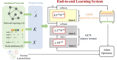
We propose an end-to-end deep learning method to combine the GCN and MRF methods for semi-supervised community detection on attribute networks. In this new method, we cast the MRF model to a new convolutional layer and incorporate it as the last layer of the GCN model. We then train the whole integrated model altogether, so that the semantic information used in the GCN model can be exploited in the MRF model and the latter can refine the coarse community result. To this end, we first extend NetMRF to eMRF (extended MRF) by adding unary poten-tials and content information, and by reparameterizing the MRF model in order to make it fit to the GCN architecture. We use mean field approximation for model inference in eMRF. By doing so, we can formulate the steps of the mean field inference as a series of convolution operations, and thus convert eMRF into a convolutional layer of GCN. The integrated GCN and converted eMRF constitute an end-to-end deep CNN (Fig. 1). In this end-to-end model, the last convolutional layer (i.e., eMRF) can refine the coarse output from the previous layers in the forward pass, and meanwhile, it can back propagate during training the differential error to the GCN layers to update their parame-ters, thus achieving a truly end-to-end integration of the GCN and MRF methods.

2. Preliminaries

2.1 Notations and the Problem

Consider an undirected and attributed network G = (A, X) specified by an n×n adjacent matrix A over n nodes and an

n×m attribute (content) matrix X of m attributes per node. There are e edges in G. Some but not all of the nodes are known to belong to some communities, which are indexed by a set of k labels {l1, l2,…,lk}. In other words, network G is partially labeled. The problem of semi-supervised com-munity detection is then to label the rest unlabeled nodes in

G, and as a result to form k communities of nodes.

2.2 Graph Convolutional Networks

Spectral Graph Convolutional Neural networks (GCN) as a type of CNN was proposed by (Bruna et al. 2014) to ana-lyze graph data. Following spectral graph theory (Chung 2010), a network can be considered as a signal x in the time domain, and transformed to the frequency or spectral domain by the graph Fourier transformation UTx, where U

is the matrix of eigenvectors of the normalized graph La-placian L defined as L In D 1/ 2AD 1/ 2 U UT

− −

= − = Λ , where

In is the identity matrix, D the matrix of nodedegrees, and

function of diagonal matrix g_θ( )Λ of L’s eigenvalues. The spectral graph convolution can then be performed as:

( ) T

g_θ*x=Ug_θ Λ U x (1) where x is a network represented by a vector of n scalars, each of which consists of the attributes of a node, and UT(.) and U(.) represent the graph Fourier transformation and inverse graph Fourier transformation, respectively.

Because the Eigen-decomposition of L is complicated and requires O(n2) time, (Defferrard et al. 2016) suggested to use the k-th order Chebyshev polynomial expansion

( )Λ

k

T  (

~

max

(2 λ ) In

Λ = Λ − and λmax is the largest eigenvalue of L) to approximate g_θ( )Λ to reduce the complexity to O(e), that is, '( ) 0 ' ( )~

K k k k

g_θ Λ ≈

∑

₌ θ T Λ where θ'k is the k-th

Chebyshev coefficient. Substituting it into formula (1) and using L~ =（2λmax）L−In, we have

~

' 0 ' ( )

K k k k

g_θ *x≈

∑

₌θ T L x. Furthermore, (Kipf and Welling 2016) proposed to use k

= 1 and λmax=2, and derived a simplified graph

convolu-tion operaconvolu-tion of GCN:g_θ*x≈θ(I_n+D−1/ 2AD−1/ 2)xwhere

θ is the only Chebyshev coefficient left. By defining

1/ 2 1/ 2

ˆ

A=D− AD− (here A = +A I_n and Dii =

∑

jAij

  _{), the}

final output for the assignment of node labels is:

(0) (1)

ˆ ˆ

( , ) softmax( ReLU( ) )

Z= f X A = A AXW W (2) where W(0) (W(1)) and ReLU (Softmax) are weight parame-ters and the activation function, respectively, in the first (and second) convolutional layers. The Adam optimizer and back-propagation are used to train the GCN model.

2.3 Network-specific Markov Random Fields

Markov Random Fields (MRF), an undirected probabilistic graphical model, has been successfully used to solve many problems such as image segmentation (Feng et al. 2010; Zheng et al. 2015). A complete MRF model is represented by an energy function, consisting of unary potentials

( u) i iφ y

∑

and pairwise potentials ( u, v) i j i j≠ψ y y

∑

. The

unary term (φ yiu)for an individual i measures the cost that it has label u. The pairwise term ( u, v)

i j

y y

ψ for i and j rep-resents the cost that they have labels u and v, respectively. We recently extended MRF to community detection (He et al. 2018). The difficulty of using MRF for a graph prob-lem is how to define pairwise potentials ( u, v)

i j i j≠ψ y y

∑

,

which is the main focus of the work in (He et al. 2018) without considering the unary potentials. Our network-specific pairwise MRF (NetMRF) is to 1) reward the edges between nodes in the same community, 2) penalize the edges across different communities, 3) penalize missing edges (nonedges) between nodes in the same community, and 4) reward nonedges across different communities. The pairwise potential between nodes i and j is then defined as

( )

( u, v) ( 1) u,v( 2 )

i j i j ij

y y d d e a

ψ _{= − −} δ _{− (3)}

where aij=1, if there is an edge between nodes i and j, or 0, otherwise, di is the degree of node i, u and v are communi-ty labels of i and j, respectively, and δ( , )u v equals to 1, if

u=v, or 0, otherwise. A network-specific belief propagation algorithm was introduced to learn the NetMRF model.

3. The Method

3.1 Overview

Our new approach falls into the framework of GCN with a MRF model being added as a new convolutional layer (Fig. 1), so we named it as MRFasGCN. The central piece of the new method is a transformation of a MRF model and its inference to a convolutional layer to be added as the third (the last) layer to the original two-layer architecture of GCN (Fig. 1). By doing so, we are able to integrate and train these two types of models together to develop a truly end-to-end deep learning method for community detection.

Fig. 1. The MRFasGCN architecture. Given an attribute network

with adjacency matrix A and node attribute matrix X, the renor-malized adjacent matrix A of A and the similarity matrix of ˆ nodes K based on A and X are calculated in advance, which are used as the inputs of the neural network along with X. MRFasGCN is composed of three convolution layers. The first two layers are from GCN which use A to convolve the attribute ˆ matrix X. The result of the first two layers is a coarse community labeling. The third convolutional layer performs the MRF infer-ence to refine the result from the first two layers. The final output is obtained by subtracting the refined result from GCN’s result. The model is trained via the Adam optimizer which calculates gradients to update weight parameters (i.e., W(2), W(1) and W(0)).

third convolutional layer (i.e., MRF) requires probabilistic community memberships, we use Softmax as the activation function in the second layer.

The third convolutional layer, which is designed for MRF, is the most important part of our MRFasGCN. It is to take advantage of the MRF’s pairwise potentials to make the new model community oriented and to perform a smooth refinement to the coarse results from GCN. To this end, we extend NetMRF to eMRF as follows. First, to let eMRF handle the results from GCN, we add unary poten-tials, attribute information and trainable weight parameters. The unary potentials are used to link the MRF layer to GCN, i.e., the output of the previous convolutional layer from GCN, i.e., X(2), are taken as an initial value of the unary potentials as a preliminary assignment of communi-ties. To incorporate attribute information, we then compute a similarity matrix of nodes K based on network topology and node attributes (introduced in later sections), instead of using the original similarity matrix based on the topology alone. We then add weight parameters W(2) to better de-scribe communities, which depict latent similarity relation-ships between communities. Second, we adopt a mean filed approximation for inference in eMRF and formulate it as a convolution operation, which is represented as KX(2)W(2). The activation function of the third layer ensures that the output is a set of probabilistic community memberships.

The overall end-to-end deep neural network is trained by the Adam optimizer (Kingma and Ba 2015), a well-known optimizer for deep learning. The loss function is the cross entropy loss between the predicted community labels and the partial ground-truth labels.

3.2 Formulation of MRF as GCN

This is the key to our method. We first extend NetMRF to eMRF to be integrated with GCN, then use a mean filed approximate for model inference and finally formulate eMRF as a convolution layer to form MRFasGCN.

3.2.1 The eMRF Model

In order to extend NetMRF (He et al. 2018) to eMRF, we introduce unary potentials, weight parameters and attribute information to the new model. The unary potentials are used to connect with GCN. Since the unary potential

( u)

i y

φ measures the cost of node i having label u, we use

(yui) p y( iu)

φ = − , where p y( iu) is the probability that node i

has label u whose inital value comes from GCN’s result. For pairwise potentials, we note that (He et al. 2018) only consider the topological difference between intra- and in-ter-community relationships, but ignore the semantic simi-larities between communities that may also be critical for community detection. For example, a ‘politics’ community is more similar to an ‘economy’ community than a ‘sports’ community. To solve this issue, we add weight parameters

(2) u,v

W to the pairwise potential of NetMRF to revise the pairwise potential to

(yiu,yvj) ( , ) ( , )u v b i j

ψ′ =µ (4) whereb i j( , )=d di j/2e a− ijas before,

( , ) ( 2)

, ( , )u v ( 1) u vWu v

µ _{= −} δ

in which ( , ) ( 1)₋ δu v

can be seen as the prior of µ( , )u v and

( 2 )

,

u v

W represents the trainable similarity relationship be-tween communities of nodes i and j.

Note that the similarity potential b(i, j) was originally defined based on network topology alone in NetMRF. We further extend it to incorporate attribute information. Spe-cifically, we first use the cosine similarity

T

) / (

( , xi xj |xi| | j|)

s i j = ⋅ ⋅ x between the node attributes of nodes i and j to measure their similarity, where xi is the i-th row of attribute matrix X. To properly define every node’s similarity, we introduce an asymmetric regularization term to balance the difference of the sum of similarity on every node, i.e.,

1

( ( , )) ( , ) / n ( , )

i _t

R s i j =s i j

∑

₌ s i t . Combining the topology and attribute information, the similarity between nodes i and j is

T

( , ) ( , ) * (_{i i j} / (| _i| | _j|))

k i j =b i j +β R x x⋅ x ⋅ x (5) where β is a parameter to make a tradeoff between network topology and attributes, which can be set to 1 when no prior is available. The final pairwise potential is

(y_iu,yv_j)= ( , ) ( , )u v k i j

ψ′′ µ ₍₆₎

Let C = (C1,C2,…,Cn) be a partition of network G, where

Ci denotes the community label to which node i belongs. Then, the final energy function of eMRF is defined as

( , ) ( _iu) ( , ) ( , )

i i j

E C | A X =

∑

−p y +α

∑

_≠ µ u v k i j (7) where α is the parameter to make a tradeoff between the unary and pairwise terms which can also be set to 1 gener-ally. The weight parameters W(2) can be learned in model training. The similarity propensities of nodesK=( ( , ))k i j _{n n×} can be calculated using (5) based on both network topolo-gy and attribute information. In (7), ( u)

i

p y comes from the result of GCN, so that the unary terms

∑

i−p y( ui) serve as

an interface between GCN and MRF, and consequently eMRF can be included in the GCN architecture.

3.2.2 Mean Field Approximate for eMRF’s Inference To retrofit the eMRF model into GCN paradigm, we for-mulate the model fitting procedure of MRF by proper con-volution operations. The pairwise part of eMRF’s energy function in (7) is fully connected. As a result, the exact distribution P(C | A, X) is difficult to compute. We use mean field approximate inference to derive a decomposa-ble iterative update equation for P(C | A, X), making it fea-sible to be formulated as suitable convolution operations.

In mean field inference, we replace the exact probability distribution P(C) (denoting P(C | A, X) for short) with an approximate distribution Q(C) that is used to minimize the KL-divergence D(Q || P). Here, Q(C) is decomposable, i.e.,

( ) i i( i)

Q C =

∏

Q C . For simplicity, we use EU~Q to denote the expected value under distribution Q. We can then write

~ ~

distribution is 1 Z

( | , )= exp( ( | , ))

P C A X −

∑

E C A X , so

~ ~

D( || )Q P =E_{U Q}[ ( )]EU +E_{U Q}[log ]Z +E_U~Q[log ( )]QU ,(here

Z is a normalized constant). Because Q C( )=

∏

_iQ C_i( _i), we have _~ [log ( )] _~ [log( ( ))]

i i i i

Q Q =

∑

i U Q Q U U

E U E and then

~ ~

D( || ) [ ( )] [log ( )] log

i i

Q i U Q i i

Q P =EU EU +

∑

E Q U + Z (8) To optimize Qi(Ci), we define a Lagrangian that consists of all terms in D(Q || P) that involve Qi(Ci), i.e.,

~

( ) [ ( )] ( ) log ( )+ ( ( ) 1)

i Q i i i i i i i

L Q =EU E U +Q C Q C λ

∑

Q C − (9) where Lagrange multiplier λ corresponds to the constraint that assures all Qi(Ci) to be probability distributions. We now take derivatives on (9) with respect to Qi(Ci):

~

( ) / ( ) [ ( ) | ] log ( ) 1

i i i Q i i i

L Q Q C E C Q C λ

∂ ∂ =E_U U + + + (10)

where EU~Q[ ( ) |E U Ci]= (φ Ci)+

∑

j i≠EUj~Qj[ ( ,ψ C Ui j)] . By setting derivative to 0 and reordering all terms, we have

~

logQ Ci( i)= −(λ+1)−EU Q[ ( ) |E U Ci] (11) As λ+1 is a constant relative to Ci and can be calculated by renormalization, the final formula for Qi(Ci) is then

1

( ) exp{ ( ) [ ( , )]}

j j i

i i Z i j i Q i j

Q C = −φ C −

∑

_≠E_U ψ C U (12) Substituting ( u, v)

i j

y y

ψ′′ of (6) into (12), we have

1 1

( ) exp{ ( ) [ ( , ) ( , )]} = exp{ ( ) ( ) ( , ) ( , )}

j j i

i j

i i Z i j i Q i j

i j j i j

Z j i C L

Q C C C U k i j

C Q C C C k i j

φ µ

φ _≠≠ _∈ µ

= − −

− −

∑ ∑

∑

U

E _

(13)

After transposition, the final iterative update equation is

1

( ) exp{ ( ) ( , ) ( , ) ( )}

i j

i i Z i j i C L i j j j

Q C = −φC −

∑ ∑

_{≠ ∈} µ C C k i j Q C (14) By minimizing the KL-divergence and constraining Q(X) and Qi(Xi) to be valid distributions, we can derive

1

( ) exp{ ( ) ( , ) ( , ) ( )}

i j

i i Z i j i C L i j j j

Q C = −φC −

∑ ∑

_{≠ ∈} µ C C k i j Q C (15) 3.2.3 Incorporate eMRF’s Inference into GCN Training Based on the update equation of eMRF in (15), we formu-late it as convolution operations to finalize the last compo-nent of the integrated end-to-end deep neural network.

The update equation in (15) can be split into four steps, i.e., initialization, message passing, addition of unary po-tentials and normalization, each of which can be formulat-ed as convolutional operations. For clarity, we use Q u_i( )

to denote the approximate probability of node i having community label u and define the updated Q u_i( ) in each step as 1

( ) i Q u , 2

( ) i Q u , 3

( ) i

Q u and 4

( ) i

Q u respectively. 1. Initialization. Assume Ci = u and the initialization is done by 1_{( )} 1_{exp{ ( )}}

i

u

i Z i

Q u ← −φ y It is equivalent to apply-ing Softmax to the output of GCN, that is ( u) ( u)

i i

y p y

φ = −

. 2. Message passing. The process of message passing consists of two parts: message passing between nodes and message passing between communities. For the first one, the formula of message passing from node j to node i is

1 1

( ) ( , ) ( )

j j i j

Q u ←

∑

_≠k i j Q u . This can be taken as

multiply-ing similarity matrix K=( ( , ))k i j _{n n×} calculated in (5) by the initialized Q matrix. For the second one, the formula of message passing from community v to community u is

1 1

( ) ( , ) ( )

j j i j

Q u ←

∑

_≠k i j Q u . Because the weights ( 2)

u,v W used in μ(u,v) can be learned in training, this can also be taken as a convolution operation executed on 1

( )

i

Q u , where the receptive field of the convolution filter is 1×1, and the numbers of input and output channels are both k.

3. Addition of unary potentials. This step is carried out

by 3 2

( ) ( ( u) ( ))

i i i

Q u ← −φ y +Q u , which is equal to adding a unary term to Q ui2( ) and then take its negative number.

4. Normalization. The last step is performed as

3 2

( ) ( ( u) ( ))

i i i

Q u ← −φ y +Q u . This can be taken as applying Softmax to normalize the output from the previous step.

Following above steps, we transform the eMRF’s infer-ence into a convolution process which is compatible with GCN. By adding eMRF as the last CNN layer to the origi-nal two-layer structure, we thus integrate GCN and MRF in a joint end-to-end learning system MRFasGCN.

As we define X(1), X(2) and Z as the outputs of the first, second and third convolution layers, and W(0), W(1) and W(2)

as the weights of the first, second and third layers, respec-tively, the forward model (which denotes the model in the forward pass of our designed deep neural network) is:

(1) (0)

1( , ) Re LU(ˆ )

X = f X A = AXW ,

( 2) (1) (1) (1)

2( , ) softmax(ˆ )

X = f X A = AX W ,

(2) (2) (2) (2) 3( , , ) soft max( )

Z = f X A X = X - KX W (16)

where K=( ( , ))k i j n n× is the similarity matrix of nodes in (5), and W( 2 ) = −[( 1)δ( , )u vW_{u v}( 2 )_, ]_{k k×} . Then, MRFasGCN can be trained by minimizing the cross entropy between the predicted and the (partial) ground-truth community labels under parameters (0) (1) (2)

{ , , }

= W W W

θ , i.e.,

'

1 1

arg min ( , ) arg min( n_i k_j ijln ij)

θ L Z Y = θ −

∑ ∑

= =Y Z (17) where 'n is the number of labeled nodes and Y the prior community memberships. Then, it can be trained by using the back-propagation algorithm as done in GCNs or CNNs.

3.3 Complexity Analysis

We ran our approach on TensorFlow with an efficient GPU implementation, i.e., sparse-dense tensor multiplication. In the first convolutional layer, both Aˆ and X are sparse ten-sors, and W(0) has a shape of m×h, so that the computation-al complexity of this layer is O(emh), where h is the num-ber of hidden units of the first layer. In the second layer,

W(1) has a shape of h×k. So the computational complexity in the first two layers is O(emhk), where e, m and k are the numbers of edges, attributes and communities, respectively. In the third layer, K is a sparse tensor and W(2) has a size of

k×k. The total complexity for all three layers in (16) is O(emhk2). This time complexity is linear in the number of edges on large and sparse networks. Because we used a sparse representation for the adjacent matrix, the space complexity of our approach is O(e), which is the same with of the original GCN and is linear in the number of edges.

4 Experiments

In training, we adopted the widely-used Adam optimizer and ran experiments on TensorFlow. We set the learning rate to 0.03, the dropout rate to 0.8, and the maximum epoch to 200. We terminated the training process when the loss function failed to decrease in 10 consecutive epochs. We use the same scheme in GCN to initialize the weights of MRFasGCN’s first two CNN layers; we initialized the weights of the third layer uniformly, i.e., the weights were randomly chosen from a uniform distribution. The number of hidden units of the first convolution layer is 16 (i.e., h = 16) except for NELL (see below) which has 64 units.

4.1 Why MRFasGCN Works

4.1.1 Quantitative Analysis

To understand MRFasGCN, we compared it with GCN (Kipf and Welling 2016) and the naive two-stage scheme that we outlined earlier, i.e., running GCN first and then applying eMRF to refine its results. Note that eMRF can also run individually. We did not compare MRFasGCN with eMRF because GCN+MRF is an enhanced eMRF that uses GCN’s results to define its unary potentials.

Table 1. Datasets descriptions. Here, rate (%) denotes the pro-portion of semi-supervised information

Datasets Nodes Edges Communities Attributes Rate (%) Cornell 195 286 5 1,703 20

Texas 187 298 5 1,703 20 Washington 230 417 5 1,703 20 Wsicsonsin 265 479 5 1,703 20 UAI2010 3,363 45,006 19 4,972 3.0 Citeseer 3,327 4,732 6 3,703 3.6 Cora 2,708 5,429 7 1,433 5.2 Pubmed 19,717 44,338 3 500 0.3 NELL 65,755 266,144 210 5,414 0.1

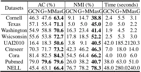
Table 2.The results of GCN, GCN+MRF (G+M for short) and MRFasGCN (MasG for short) in terms of accuracy (AC), normal-ized mutual information (NMI) and runtime.

Datasets AC (%) NMI (%) Time (seconds) GCN G+M MasG GCN G+M MasG GCN G+M MasG Cornell 46.3 47.6 63.4 9.1 14.7 38.8 2.4 5.5 3.1

Texas 57.1 55.4 71.1 5.0 5.0 45.0 2.0 5.0 2.2 Washington 54.9 58.8 70.6 16.3 23.4 41.4 1.9 4.5 2.2 Wsicsonsin 55.6 53.8 72.7 17.8 18.5 52.2 2.5 5.3 3.0 UAI2010 16.4 18.3 50.6 3.8 9.1 40.5 42.0185.2120.3

Citeseer 70.3 71.7 73.2 42.3 46.2 46.3 7.0 18.0 14.0 Cora 81.4 82.5 84.3 54.5 64.4 66.2 4.0 10.0 6.0 Pubmed 79.0 79.6 79.6 26.0 38.2 40.7 38.0 63.0 51.0

NELL 45.4 63.1 66.4 76.7 78.2 78.3 48.0280.0240.0

The datasets are shown in Table 1. Citeseer, Cora, Pub-med and NELL are from (Kipf and Welling 2016) which is used to validate GCN. The proportion of semi-supervised information that was made available was set according to

(Kipf and Welling 2016). Cornell, Texas, Washington, Wisconsin and UAI2010 are from (Wang et al. 2018) which are also used to validate community detection meth-ods. The proportion of their semi-supervised information was set according to (Wang et al. 2018). We used Accura-cy (AC) and Normalized Mutual Information (NMI) (Liu et al. 2012) as metrics for performance evaluation.

As shown in Table 2, MRFasGCN has the best perfor-mance and GCN+MRF outperforms GCN, confirming that the two-stage method GCN+MRF improves upon GCN through MRF’s refinement. This also validates that MRFasGCN improves upon GCN+MRF in an end-to-end deep learning so that their complementary features can be tightly integrated so as to find optimal or near optimal so-lutions. While GCN+MRF and MRFasGCN have roughly similar magnitudes of running time (Table 2), MRFasGCN runs faster than MRF+GCN, indicating that the integration of the two can also help speed up the process for finding the right weights for all three layers for model fitting. 4.1.2 Qualitative Analysis

To further validate the refining function of MRFasGCN’s third convolution layer, we illustrate two nodes in Cora which were mistaken by GCN but corrected by MRFasGCN in Fig. 2. Each node’s color denotes its pre-dicted community labeling. The node containing an aster-isk is labeled, otherwise is unlabeled. For node id2395 in the Fig. 2(a), it was erroneously assigned to community 7 by GCN. The reason for the mistake is that one of its neighbors is labeled and this label directly affects node id2395’s predicted label. In comparison, MRFasGCN cor-rectly assigned node id2395 to its correct community 1. This is because MRFasGCN uses the MRF layer to refine the coarse results from GCN by using information on the nodes adjacent to node id2395. We observe another node (id 572) that was also mistaken by GCN (Fig. 2(b)). In this case, supervised information misguided GCN again – node id572 was wrongly assigned to community 7 because one of its 2-hop neighbors is originally labeled as community 7. Fortunately, the pairwise potentials of MRFasGCN consid-er the label consistency between nearby nodes and correct-ly adjust this node’s label to community 4.

4.2 Comparison with the Existing Methods

We compared MRFasGCN with three types of the state-of-the-art methods. The first includes DCSBM (Karrer and Newman 2011) and NetMRF (He et al. 2018), which both use network topology alone. The second type includes PCLDC (Yang et al. 2009), SCI (Wang et al. 2016) and NEMBP (He et al. 2017), which use both topology and attribute information. The third type includes WSCDSM (Wang et al. 2018) and DIGCN (Li et al. 2018), which are semi-supervised methods on attribute networks.

Table 3. Comparison of prediction accuracy (AC). Bold font indicates the best result. ‘-’ indicates that runtime exceeds 24 hours or out-of-memory. Our method is denoted by MasG and other methods are denoted by first three characters for short.

Datasets AC (%)

DCS Net PCL SCI NEM DIG WSCMasG Cornell 37.9 31.8 30.3 36.9 47.2 46.3 53.9 63.4 Texas 48.1 30.6 38.8 49.7 53.6 57.1 77.5 71.1 Washington 31.8 35.0 30.0 46.1 42.9 50.0 58.3 70.6 Wsicsonsin 32.8 28.6 30.2 46.4 63.4 55.6 61.9 72.7 UAI2010 2.6 31.1 28.8 29.5 46.3 17.3 27.2 50.6 Citeseer 26.6 22.2 24.9 34.4 49.5 70.1 47.6 73.2 Cora 38.5 58.1 34.1 41.7 57.6 81.7 53.7 84.3 Pubmed 53.6 55.5 63.6 - 65.7 79.2 - 79.6

NELL - - - 45.2 - 66.4

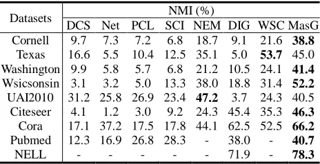
Table 4.Comparison of 8 community detection methods in NMI.

Datasets NMI (%)

DCS Net PCL SCI NEM DIG WSCMasG Cornell 9.7 7.3 7.2 6.8 18.7 9.1 21.6 38.8

Texas 16.6 5.5 10.4 12.5 35.1 5.0 53.7 45.0 Washington 9.9 5.8 5.7 6.8 21.2 10.5 24.1 41.4 Wsicsonsin 3.1 3.2 5.0 13.3 38.0 18.8 31.4 52.2 UAI2010 31.2 25.8 26.9 23.4 47.2 3.7 24.3 40.5

Citeseer 4.1 1.2 3.0 9.2 24.3 45.4 35.3 46.3 Cora 17.1 37.2 17.5 17.8 44.1 62.5 52.5 66.2 Pubmed 12.3 16.9 26.8 28.3 - 38.0 - 40.7

NELL - - - 71.9 - 78.3

Measured in AC, MRFasGCN performs the best on 8 of 9 networks and the second best on the remaining Texas networks (Table 3). In general, the methods that use both topology and attribute information perform better than those using topology alone, and the semi-supervised meth-ods outperform the ones that do not use prior membership information. We highlight that among the semi-supervised methods, MRFasGCN is on average 15.1%, 14.4% more accurate than WSCDSM and DIGCN, respectively.

The NMI results follow a similar trend as in AC (Table 4). MRFasGCN performs the best on 7 of the 9 networks, and is also competitive on the rest 2 networks. Compared with semi-supervised methods, it is 12.5% and 20.5% more accurate than WSCDSM and DIGCN on average. This further validates its effectiveness over the existing methods.

5 Related Work

First, different from images, networks are non-Euclidean in that they do not have fixed topological structures that are essential for convolution operations. Second, there is no in-depth study about MRF for community detection, the only one is our work in (He et al. 2018), whereas we ignore the information on nodes and requires a substantial amount of computation for learning the model. Third, the construction of the joint training of different types of network-specific statistical models is also a non-trivial task. We overcame these challenges and successfully developed a joint model of GCN and MRF for network community detection.

6 Conclusion

We proposed an end-to-end deep learning method, namely MRFasGCN, to integrate GCN and MRF for the problem of semi-supervised community detection in attributed net-works. It has architecture of three convolutional layers with GCN as the first two convolution layers and MRF as the third layer. The MRF component utilizes the coarse output of GCN to construct MRF’s unary potentials, and then enhances the network-specific pairwise potentials to find better communities. In addition to the integrated GCN and MRF architecture, another significant contribution of our work is the novel transformation of MRF to CNN. We analyzed and demonstrated the strength of our model in both accuracy and running time. Experimental results showed that it outperformed the state-of-the-art community detection methods on many large real-world networks.

Acknowledgments

This work was supported by National Key R&D Program of China (2017YFB1401201), Natural Science Foundation of China (61876128, 61772361, 61502334, U1736103).

References

Bruna, J.; Zaremba, W,; Szlam, A.; and Lecun, Y. 2014. Spectral Networks and Locally Connected Networks on Graphs. In Inter-national Conference on Learning Representations, Banff, Canada. Chen, Z.; Li, X.; and Bruna, J. 2018. Supervised Community Detection with Hierarchical Graph Neural Networks. arXiv pre-print arXiv: 1705.08415.

Chung, F. R. K. 1997. Spectral graph theory. Published for the Conference Board of the mathematical sciences by the American Mathematical Society 1997: 212.

Defferrard, M.; Bresson, X.; and Vandergheynst, P. 2016. Convo-lutional neural networks on graphs with fast localized spectral filtering. In Neural Information Processing Systems, 3844-3852. Barcelona, Spain.

Feng, W.; Jia, J.; and Liu, Z. Q. 2010. Self-Validated Labeling of Markov Random Fields for Image Segmentation. IEEE Transac-tions on Pattern Analysis & Machine Intelligence, 32(10): 1871.

Girvan, M.; and Newman, M. E. 2002. Community structure in social and biological networks. Proceedings of the national acad-emy of sciences 99(12): 7821-7826.

Hammond, D. K.; Vandergheynst, P.; and Gribonval, R. 2011. Wavelets on graphs via spectral graph theory. Applied and Com-putational Harmonic Analysis, 30(2): 129-150.

He, D.; Feng, Z.; Jin, D.; Wang, X.; and Zhang, W. 2017. Joint Identification of Network Communities and Semantics via Inte-grative Modeling of Network Topologies and Node Contents. In Proceedings of the 31th AAAI Conference on Artificial Intelli-gence. San Francisco, California, USA: AAAI Press.

He, D.; You, X.; Feng, Z.; Jin, D.; Yang, X.; and Zhang, W. 2018. A Network-Specific Markov Random Field Approach to Com-munity Detection. In Proceedings of the 32th AAAI Conference on Artificial Intelligence. Arlington, Virginia, USA: AAAI Press. Jia, S.; Gao, L.; Gao, Y.; Nastos, J.; Wang, Y.; Zhang, X.; and Wang, H. 2015. Defining and identifying cograph communities in complex networks. New Journal of Physics 17(1): 013044 Karrer, B.; and Newman M. E. J. 2011. Stochastic blockmodels and community structure in networks.Phys Rev E Stat Nonlin Soft Matter Phys 83: 016107.

Kingma, D. P.; and Ba, J. 2015. Adam: A method for stochastic optimization. In International Conference on Learning Represen-tations. San Diego, CA.

Kipf, T. N.; and Welling, M. 2016. Semi-supervised classification with graph convolutional networks. In International Conference on Learning Representations. San Juan, Puerto Rico.

Krähenbühl, P., and Koltun, V. 2011 Efficient Inference in Fully Connected CRFs with Gaussian Edge Potentials. In The Twenty-fifth Annual Conference on Neural Information Processing Sys-tems, 109-117. Granada Spain.

Li, Q.; Han, Z.; and Wu, X. M. 2018. Deeper Insights into Graph Convolutional Networks for Semi-Supervised Learning. Thirty-First AAAI Conference on Artificial Intelligence. San Francisco, California, USA: AAAI Press.

Liu, H.; Wu, Z.; Li, X.; Cai, D.; and Huang, T. S. 2012. Con-strained nonnegative matrix factorization for image representation. IEEE Transactions on Pattern Analysis & Machine Intelligence 34(7): 1299-1311.

Tu, K.; Cui, P.; Wang, X.; Wang, F.; and Zhu, W. 2018. Structur-al Deep Embedding for Hyper-Networks. Thirty-Second AAAI Conference on Artificial Intelligence. New Orleans, Louisiana, USA: AAAI Press.

Wang, W.; Liu, X.; Jiao, P.; Chen, X.; and Jin, D. 2018. A Uni-fied Weakly Supervised Framework for Community Detection and Semantic Matching. Pacific-Asia Conference on Knowledge Discovery and Data Mining: 218-230.

Wang, X.; Jin, D.; Cao, X.; Yang, L.; and Zhang, W. 2016. Se-mantic community identification in large attribute networks. Thir-tieth AAAI Conference on Artificial Intelligence. Phoenix, Arizo-na, USA: AAAI Press.

Yang, T.; Jin, R.; Chi, Y.; and Zhu, S. 2009. Combining link and content for community detection: A discriminative approach. In Proceedings of the 15th ACM SIGKDD International Conference on Knowledge Discovery and Data Mining, 927- 936. New York, NY: ACM Press.