The Thirty-Third AAAI Conference on Artificial Intelligence (AAAI-19)
Stochastic Submodular Maximization with Performance-Dependent Item Costs
∗Takuro Fukunaga,
1Takuya Konishi,
2Sumio Fujita,
3Ken-ichi Kawarabayashi
2 1RIKEN Advanced Intelligence Project and JST, PRESTO, [email protected]2National Institute of Informatics,{takuya-ko,k keniti}@nii.ac.jp
3Yahoo Japan Corporation, [email protected]
Abstract
We formulate a new stochastic submodular maximization prob-lem by introducing the performance-dependent costs of items. In this problem, we consider selecting items for the case where the performance of each item (i.e., how much an item con-tributes to the objective function) is decided randomly, and the cost of an item depends on its performance. The goal of the problem is to maximize the objective function subject to a bud-get constraint on the costs of the selected items. We present an adaptive algorithm for this problem with a theoretical guaran-tee that its expected objective value is at least(1−1/√4e)/2 times the maximum value attained by any adaptive algorithms. We verify the performance of the algorithm through numerical experiments.
1
Introduction
In the stochastic submodular maximization, we are given a set of items associated with a random utility function that has a certain diminishing marginal return property. The goal of the problem is to select items so as to maximize the utility function subject to constraints. To deal with decision making under uncertainty, several variants of stochastic submodular maximization are actively being considered (see Section 2), and the approaches proposed in this literature have been successfully applied to numerous decision making tasks.
The aim of this paper is to introduce the performance-dependent costsof items into the stochastic submodular max-imization. In many decision making applications, we some-times have to make a decision without exact information on the performance of each item (i.e., how much an item con-tributes to the utility function) because it varies on several uncertain factors. Moreover, it is often the case that the cost of selecting an item varies depending on its performance. To deal with this situation, we introduce random performance and performance-dependent costs of items, and consider the stochastic optimization problem of maximizing the utility function subject to a budget constraint on the costs of the selected items.
∗
The first author is supported by JSPS KAKENHI Grant Number JP17K00040 and JST PRESTO Grant Number JPMJPR1759. The second and the fourth authors are supported by JST ERATO Grant Number JPMJER1201.
Copyright c⃝2019, Association for the Advancement of Artificial Intelligence (www.aaai.org). All rights reserved.
This problem models many natural settings of decision making. Here, we present two examples.
Recommendation:Diminishing marginal return property plays a key role in designing objectives for recommender systems (Ziegler et al. 2005). For example, in news recom-mendation, users often browse news articles in order to cover daily news or to know the different aspects of a favorite topic. It is critical for such users to recommend diverse and unseen items, and the objective function is modeled through submod-ular functions (El-Arini et al. 2009; Yue and Guestrin 2011; Ahmed et al. 2012). In several practical scenarios, the per-formance of a recommended item is determined by some random factors, and it incurs a cost according to the per-formance; e.g., when a user receives recommended news articles, he/she decides to skip or (partially) read them and spends his/her own time or money by reading the selected articles. The existing formulations are not applicable to this situation because they cannot deal with the case where both the performances and the costs of items are unknown before recommending them.
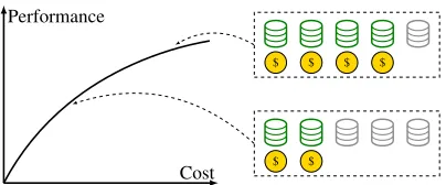
Batch-mode active learning: In the batch-mode active learning, we have a set of unlabeled data and the objective is to select several data points to label subject to a budget constraint on the cost. In a previous study (Hoi et al. 2006), this task is formulated as a monotone submodular maximiza-tion problem, where the objective funcmaximiza-tion represents the information amount of data. However, this existing formu-lation does not consider uncertainty in the performance of labeling. In many cases, time for labeling the given data is limited, and it is uncertain in advance how much data can be processed within the given time due to factors such as variation of labelers’ skill and experimental conditions. Also, it is natural that the cost (e.g., the fee paid to labelers) for the labeling depends on the amount of processed data (see also Figure 1). Our problem can model this situation while it cannot be handled by the existing formulation.
We present algorithms that compute adaptive policies for this problem together with the theoretical analysis of their performances. One of our proposed algorithms is guaranteed to achieve an expected objective value of least(1−1/√4e)/2
$ $ $ $ $ $
Cost Performance
Figure 1: An illustration of the performance-dependent cost of an item in the batch-mode active learning. In this figure, an item corresponds to a group of data points and each cylinder denotes one data point in a group. Once the number of the processed data points is revealed, the corresponding expense is incurred.
perform better than baseline algorithms in many settings. For example, when the algorithms are applied to a task of the batch-mode active learning, we observe that our algorithms reduce the prediction errors of a learning algorithm compared with baseline algorithms; see Section 6 for more details.
Our algorithms extend the algorithm of Gupta et al. (2011) for a stochastic knapsack problem, which corresponds to a special case of our problem where the objective function is linear. Since the performance guarantee of Gupta et al. is
1/8 = 0.125, our guarantee is not much worse than it al-though our algorithms deal with a more general problem; relationships with previous studies are discussed more in Section 2. Except for our algorithms, we are aware of no algorithms that achieve a constant approximation ratio for our problem. It is important to observe that the ratio is a con-stant because it means that the algorithm behaves reasonably for any instance. Indeed, numerical experiments show that the empirical performance of our algorithms is stable while baseline algorithms sometimes achieve only small objective values; in a certain instance, the scores of baseline algorithms are less than 70% of our proposed algorithms.
Our algorithms are based on the contention resolution scheme, which is a general framework to design approxi-mation algorithms for the submodular maximization. The contention resolution scheme is so useful that many efficient algorithms based on it have been proposed in the literature. However, the existing scheme is not applied to our problem because it is restricted to the submodular set-functions. In our problem, the objective function is defined over the integer lat-tice in order to represent the dependence of the objective on the performance levels of selected items. Thus, we extend the contention resolution scheme to lattice-submodular functions, and design our algorithms based on this extended framework. This technique is potentially useful in other contexts, and so it is of independent interest.
To summarize, the contributions of this paper can be de-scribed as follows.
• We formulate a new stochastic submodular maximization by introducing the performance-dependent costs of items, which has numerous natural applications.
• We present adaptive algorithms for the above problem, one of which has the theoretical guarantee that its expected
objective value is at least(1−1/√4e)/2times the
opti-mal value. Its empirical performance is verified through numerical experiments.
• To design the algorithms, we extend the contention res-olution scheme to lattice-submodular functions, which is a new general framework of independent interests to design approximation algorithms for maximizing lattice-submodular functions.
The remainder of this paper is organized as follows. Sec-tion 2 reviews related previous studies. SecSec-tion 3 formulates our problem. Our algorithms and their analysis are given in Sections 4 and 5. Since our algorithms are based on a contin-uous relaxation of the original problem, Section 4 formulates this continuous relaxation and discusses how to solve it. Sec-tion 5 explains how to construct an adaptive policy from a continuous solution. Section 6 reports on numerical experi-ments, and Section 7 concludes the paper.
2
Related Work
Since the body of previous studies on submodular maximiza-tion is huge, we here review some of those on its stochastic variants. A typical example of stochastic submodular max-imization is the study of Golovin and Krause (2011) on adaptive submodularity. They proposed the notions of adap-tive submodularity and adapadap-tive monotonicity of stochas-tic set-functions, and presented an adaptive algorithm for maximizing adaptive monotone submodular functions. Since their study, adaptive algorithms for maximizing adaptive submodular functions have been investigated in various set-tings (Chen and Krause 2013; Fujii and Kashima 2016; Gabillon et al. 2013; Gabillon et al. 2014; Gotovos, Karbasi, and Krause 2015; Yu, Fang, and Tao 2016).
Another example of stochastic submodular maximization is the submodular probing problem (Adamczyk, Sviridenko, and Ward 2016; Gupta, Nagarajan, and Singla 2017). In this problem, the given submodular function is deterministic but each item takes the active or inactive state randomly. A cho-sen item contributes to the objective value only when it is active. The constraints consist of inner and outer constraints, where the inner constraints restrict the chosen active items, whereas the outer constraint restricts all chosen items. Thus, the inner constraints depend on the states of the chosen items, which as far as we know, is the only example where random-ness in both the objective function and the constraints are correlated as our problem.
When the objective function is linear, our problem coin-cides with the stochastic knapsack problem studied by Gupta et al. (2011). Gupta et al. gave a pseudo-polynomial time algo-rithm with the performance guarantee of ratio1/8(= 0.125). Observe that the ratio(1−1/√4e)/2(>0.110) of our
algo-rithm is not much worse than the ratio of Gupta et al. even though our algorithm is for a more general problem. Indeed, our algorithm is equivalent to the algorithm of Gupta et al. when the problem is restricted to their problem. Gupta et al. also showed that their algorithm can be converted into a polynomial-time algorithm with a constant loss of approx-imation ratio. This conversion can be also applied to our algorithm although we do not focus on it in this paper. The algorithm of Gupta et al. was later improved by Ma (2014), who gave a pseudo-polynomial time algorithm with ratio1/2. The conversion to a polynomial-time algorithm cannot be applied to the algorithm of Ma.
3
Setting
First, we introduce the lattice-submodular functions. LetZ+
andR+denote the sets of nonnegative integers and
nonneg-ative real numbers, respectively. For n ∈ Z+, we let[n]
denote{0,1, . . . , n}. LetIbe a set of items, and letB ∈Z+.
For two vectorsu, v∈[B]I,u≤vmeans that the relation holds componentwise, i.e.,u(i)≤v(i)for alli∈I.u∧v
andu∨vare the vectors in[B]I defined by(u∧v)(i) = min{u(i), v(i)}and(u∨v)(i) = max{u(i), v(i)} for all
i ∈ I. Fori ∈ I, let χi denote the vector in [B]I such that χi(i) = 1and χi(i′) = 0 for alli′ ∈ I \ {i}. Let
f: [B]I → R+ be a function over the integer lattice[B]I.
Function f is called monotoneif f(u) ≤ f(v) holds for anyu, v ∈ [B]I such that u ≤ v, andf is called lattice-submodulariff(u) +f(v)≥f(u∧v) +f(u∨v)holds for all u, v ∈ [B]I. The latter condition is equivalent to
f(u∨jχi)−f(u) ≥ f(v∨jχi)−f(v)holding for any
u, v ∈ [B]I such that u ≤ v,i ∈ I, andj ∈ [B]. Note that the lattice-submodularity does not imply the property called DR-submodularity, which is the diminishing marginal returns along the direction ofχi for eachi ∈ I. That is,
f(u+χi)−f(u)≥f(v+χi)−f(v)does not necessarily hold for allu, v∈[B]I such thatu≤vandi∈Ieven iff
is lattice-submodular.
We now formulate our new submodular optimization prob-lem, which we call thecorrelated stochastic submodular maximization problem(CSSMP). In CSSMP, we assume that each item i ∈ I has a state θ(i) ∈ {1, . . . , B}, which is independently determined at random. Letpi(j)denote the probability that the level of an item i is j, where we as-sume without loss of generality thatpi(j)>0holds for all
j ∈ {1, . . . , B}. The state of an item represents its perfor-mance level; asθ(i)is larger, the performance of itemiis better. The performance level of an item determines its cost and contribution to the objective value. We letci(j)denote the cost of an itemiwhen the state ofiisj. We assume that
ciis monotone as follows, indicating that the cost of itemiis larger as the performance ofiis better.
Assumption 1. 0 ≤ ci(1) ≤ ci(2) ≤ · · · ≤ ci(B) ≤ C
holds for anyi∈I, whereCis the given budget.
For S ⊆ I, letθS denote the vector in[B]I such that
θS(i) = θ(i) if i ∈ S, and θS(i) = 0 otherwise. The objective function of our problem is a monotone lattice-submodular functionf: [B]I →
R+, and the objective value
of our choiceSof items is defined asf(θS). Thus, if a chosen item performs well, then a better objective value is achieved. Summarizing, the inputs of CSSMP are a setIof items, a monotone lattice-submodular functionf: [B]I →R+, a
budgetC∈Z+, and the costsci:{1, . . . , B} →Z+and the
probabilitiespi:{1, . . . , B} →[0,1]associated with each itemi∈ I. The objective of CSSMP is to findS ⊆Ithat maximizesf(θS)subject to∑i∈Sci(θ(i))≤C. Recall that
θis a random vector decided by the probabilities{pi:i∈I}. Adaptive policy Our aim is to compute an efficient policy for CSSMP. A policy chooses items sequentially and receives feedback by observing the performance of the chosen items. We will now explain more concretely. We assume that the dis-tributions determining the states (or performances) of items are known to the policy but that the realizations of the states are not given beforehand. When a policy chooses an item
i∈I, its stateθ(i)(which the policy observes) is determined according to the probability distributionpi. The subsequent behavior of anadaptivepolicy can depend on the observa-tions made up to that point, whereas a policy is said to be
non-adaptivewhen the subsequent behavior is independent of observations.
In this paper, we consider the situation where the cancella-tion of items is prohibited. That is, once a policy chooses an item, this choice is irrevocable. In addition, we also prohibit the total costs of selected items from exceeding the budget. This means that we assume the following.
Assumption 2. If a policy has already selected a setSof items andci(B)> C−∑i′∈Sci′(θ(i′))for some itemi∈
I\S, then the policy cannot select itemi.
We use a vectorr ∈ [B]I to describe the behavior of a policy. If an itemi∈Iis chosen by the policy and the state ofiis realized asθ(i), thenr(i) =θ(i). Ifi∈Ihas not been chosen yet, thenr(i) = 0. We call this vector arealization vector. For a policyπand a realization vectorr∈[B]I, let
ωπ(r)∈[0,1]denote the probability that the final state of the policyπisr(i.e.,πchooses each itemi∈ {i′∈I:r(i′)>
0}, and the state of that itemiis realized asr(i)). We note thatωπ(r)reflects the randomness of bothπand the states of items whenπis a randomized policy. Letfavg(π)denote
∑
r∈[B]Iωπ(r)f(r), i.e., the average objective value attained byπ. We evaluate the performance of a policyπbyfavg(π). Our aim is to find a policyπfor whichfavg(π)is as high as possible. We say thatπis anα-approximation policyfor
α∈[0,1]iffavg(π)≥αfavg(π∗)holds for any policyπ∗.
4
Continuous Optimization Phase
4.1
Formulation of Continuous Optimization
Problem
In this subsection, we define our continuous optimization problem. Before presenting it, we first define a submodular set-functionf¯: 2I →
R+from a lattice-submodular function f: [B]I → R+. LetS ⊆I. We randomly sample a vector r∈[B]Ias follows. The components ofrare determined in-dependently. Ifi∈S, then the corresponding componentr(i)
takes a value from{1, . . . , B}, andr(i) =jwith probability
pi(j). Otherwise,r(i) = 0. We letpS(r)denote the proba-bility thatr∈[B]I is sampled. We letr ∼p
S denote that vectorris sampled according to the distributionpS. Then, we definef¯(S) =Er∼pS[f(r)]for anyS ⊆I. Iff is
mono-tone lattice-submodular, thenf¯is monotone set-submodular (Asadpour and Nazerzadeh 2016).
The continuous optimization problem is based on the con-cept of time. We assume that, if an itemiis selected, then this selection uses timeci(θ(i)). In other words, if itemiis selected at timet, then the processing oficontinues until timet+ci(θ(i)), after which the policy can choose the next item. At time0, the policy has selected no items. We regard the budgetCas the time limit. Because of Assumption 2, the policy cannot choose itemiif the processing ofimay not finish before timeC.
A variable x(i, t) ∈ [0,1] is defined for each i ∈ I
andt ∈ [C]. This variable indicates whether itemiis se-lected at timet. Letx¯ denote the vector inRI+defined by
¯
x(i) = ∑
t∈[C−ci(B)]x(i, t). Our continuous optimization
problem includes a constraintx¯(i)≤1for eachi∈I. De-fineF¯: [0,1]I →
R+as the multilinear extension off¯, i.e.,
¯
F(y) = ∑
S⊆I ∏
i∈Sy(i) ∏
i′̸∈S(1 −y(i′)) ¯f(S) for any
y ∈ [0,1]I. LetP be the set ofx ∈ [0,1]I×[C] satisfying
¯
x(i)≤1for alli∈I, and
∑
i∈I
E[min{ci(θ(i)), t}] ∑
t′∈[t]
x(i, t′)≤2t (1)
for all t ∈ {1, . . . , C}. Here, the expectation
E[min{ci(θ(i)), t}] is taken with respect to distri-bution pi. In other words, E[min{ci(θ(i)), t}] = ∑B
j=1pi(j) min{ci(j), t}. Then, our continuous opti-mization problem can be written as
max{F¯(¯x) :x∈P}. (2)
Although we definex(i, t)even fort > C−ci(B), this is only for notational convenience. Since it does not contribute to the objective function, the objective value does not de-crease even if it is set to 0. Thus we assumex(i, t) = 0for
t > C−ci(B)in the remainder of this paper.
Note that (2) containsΩ(|I|C)variables andΩ(|I|+C)
constraints. Since the budgetCis encoded inO(logC)bits, the formulation size of (2) is not polynomial but pseudo-polynomial on the input size. Due to this, our algorithm based on (2) is a pseudo-polynomial time algorithm. We can convert the algorithm into a polynomial-time algorithm with a constant loss of approximation ratio by applying the technique used in (Gupta et al. 2011) but we instead focus on the current form. Evaluating the functionF¯can be also done
by sampling in polynomial time with an error of factor1 +ϵ
for any constantϵ >0. This is standard in the submodular maximization, and see e.g., (Asadpour and Nazerzadeh 2016) and (C˘alinescu et al. 2011). In the rest of this section, we assume thatFcan be evaluated exactly for ease of discussion.
In the following theorem, we relate the optimal value of the continuous optimization problem to the maximum expected objective value attained by any adaptive policy. This enables us to compare adaptive policy based on this continuous opti-mization problem with an optimal adaptive policy.
Theorem 1. The optimal value of (2)is at least(1−1/e)·
favg(π∗)for any adaptive policyπ∗.
This theorem is proven by the validity of constraints proven by Gupta et al. (2011) and the relationship betweenF¯ and the expected objective values achieved by adaptive policies given by Asadpour and Nazerzadeh (2016).
4.2
Algorithms for the Continuous Optimization
Problem
To solve the continuous optimization problem (2), we have two choices: one is the continuous greedy algorithm, which was proposed by C˘alinescu et al. (2011) and was slightly extended by Feldman (2013); the other is the stochastic con-tinuous greedy algorithm proposed by Asadpour and Naz-erzadeh (2016).
Continuous Greedy This algorithm is for maximizing the multilinear extensionGof a monotone set-submodular func-tiongover a solvable downward-closed polytope. Here, a polytope Qis said to besolvableif there is an algorithm that optimizes linear functions over it, and is said to be
downward-closedif 0 ≤ y ≤y′ ∈ Qimplyy ∈ Q. The algorithm is controlled by a parameter called stopping time. Feldman (2013) observed that, if the continuous greedy al-gorithm with stopping timeb > 0 is applied to the prob-lem with a solvable downward-closed polytopeQ, then the algorithm outputs a solution x such that x/b ∈ Q and
G(x) ≥ (1−e−b −O(n3δ)) max
y∈QG(y)hold, where
nis the size of the set over whichgis defined andδis the step size used in the algorithm. HereQis assumed to include the characteristic vector of every singleton set. Stopping time
b should be set to1 for computing a feasible continuous solution attaining a better objective value. However, when the continues greedy algorithm is combined with a round-ing algorithm, we sometimes obtain a better performance guarantee by settingbto a value smaller than 1.
It is not obvious that the continuous greedy algorithm can be applied to our continuous optimization problem (2). This is because the objective functionF¯(¯x)(defined over the domain
[0,1]I×[C]) does not seem to be the multilinear extension of
a submodular set-function onI×[C]. Nevertheless, we can claim that this earlier analysis is valid even for our prob-lem (2), because the probprob-lem is equivalent to maximizing
¯
F(y)subject toy ∈Q:={y′ ∈[0,1]I:∃x∈P, y′ = ¯x}. Notice thatQis a downward-closed solvable polytope in
Theorem 2. If the continuous greedy algorithm with stop-ping timeb ∈ (0,1]and step sizeδ = o(|I|−3)is applied
to Problem(2), then it outputs a solutionx∈bP such that
¯
F(¯x)≥(1−1/e)(1−e−b−o(1))favg(π∗)for any adaptive
policyπ∗.
Let us sketch how the continuous greedy algorithm com-putes a solution for (2). The algorithm first initializes all variables in the temporary solutionxto 0 and then updates them by repeating the following two steps:
Step (i): find a vectordmax ∈ P that maximizesw⊤dmax
for the weight vectorw ∈ RI+×[C] defined byw(i, t) =
¯
F(¯x∨χi)−F¯(¯x)for each(i, t)∈I×[C];
Step (ii): move the current solutionxin directiondmaxby
step sizeδ∈(0,1](i.e.,xis updated tox+δdmax).
When the stopping time isb∈(0,1], the algorithm outputsx
after repeating these stepsb/δtimes.
Stochastic Continuous Greedy Theorem 2 states that us-ing the continuous greedy algorithm to solve (2) imposes two factors, one coming from the gap between (2) and the optimal objective value, and the other being due to the performance of the continuous greedy algorithm. By using the stochastic continuous greedy algorithm, we can save the former factor. The difference between the continuous greedy and the stochastic continuous greedy algorithms is the weight vector used for decidingdmax. Here, we define the weight vectorw′
used in the stochastic continuous greedy algorithm. Letr∈ [B]I be a random vector such thatr(i) = j ∈ {1, . . . , B} with probability x¯(i)pi(j) and r(i) = 0 with probability 1−x¯(i)for eachi ∈ I, where the different components are determined independently. Moreover, for eachi ∈ I, choose one integerjrandomly from{1, . . . , B}according to probability pi(j), and define the vectorri′ ∈ [B]I by
r′i(i) = max{r(i), j}andri′(i′) =r(i′)for eachi′∈I\ {i}. The value ofw′(i, t)is defined asE[f(ri′)−f(r)]for each
(i, t)∈I×[C];w′(i, t)takes the same value for allt∈[C]. We note that, ifri′(i)is defined asj, then this weight vector coincides withwused in the continuous greedy algorithm. The stochastic continuous greedy algorithm usesw′instead ofwin Step (i) of each iteration. The other part of the algo-rithm is the same as the continuous greedy algoalgo-rithm.
Asadpour and Nazerzadeh (2016) proved that the stochas-tic continuous greedy algorithm with stopping timeb = 1
outputs a solution of value at least(1−e−1−o(1))f
avg(π∗).
Note that this bound is better than that of the continuous greedy algorithm by the factor1−e−1. Their analysis can be
extended to an arbitrary value of the stopping time as follows (we skip the proof because the extension is straightforward).
Theorem 3. If the stochastic continuous greedy algorithm with stopping timeb∈(0,1]and step sizeδ =o(|I|−3)is
applied to Problem(2), then the algorithm outputs a solution
x∈bPsuch thatF¯(¯x)≥(1−e−b−o(1))favg(π∗)for any
adaptive policyπ∗.
5
Rounding Phase
This section presents an algorithm that outputs an adap-tive policy achieving at least half the objecadap-tive value of
the continuous solution. For this, we introduce the con-tention resolution scheme for lattice-submodular functions. The existing contention resolution scheme is a general frame-work that provides a rounding algorithm for maximizing set-submodular functions (C˘alinescu et al. 2011; Feldman 2013; Feldman, Naor, and Schwartz 2011). We extend this scheme to the lattice-submodular functions, and show that the solu-tion constructed by our policy coincides with the solusolu-tion output by a contention resolution scheme. Since the con-tention resolution scheme for set-submodular functions is widely used in the literature, our extension is of independent interest.
5.1
Contention Resolution Scheme for
Lattice-Submodular Functions
The considered setting is defined as follows. Letf: [B]I → R+be a monotone lattice-submodular function and the
prob-ability distributionqi: [B]→[0,1]on[B]be given for each
i∈I. We writev ∼qifv∈[B]I is a random vector such that, for eachi ∈ I, the corresponding componentv(i)is determined independently asj∈[B]with probabilityqi(j). LetF ⊆[B]I be a downward-closed subset of[B]I(i.e., if
u ≤ v ∈ F, thenu∈ F), and letα ∈ [0,1]. A mapping
ψ: [B]I → Fis referred to as anα-contention resolution
scheme(α-CRS) with regards toqif it satisfies the following two conditions:
(i) ψ(v)(i)∈ {v(i),0}for eachi∈I;
(ii) ifv∼q, thenPr[ψ(v)(i) =j |v(i) =j]≥αholds for eachi∈Iandj ∈B, where the probability considers the randomness ofv as well as that ofψwhenψis a random mapping.
Anα-CRSψis said to bemonotoneif, for eachu, v ∈ [B]Isuch thatu(i) =v(i)andu≤v,Pr[ψ(u)(i) =u(i)]≥ Pr[ψ(v)(i) =v(i)]holds, where the probability here consid-ers only the randomness ofψ.
We prove that a monotoneα-CRS mapsv ∈ [B]I into a vector inF, for which the value off is at leastαtimes that forvin expectation. The proof requires the following preliminary lemma, known as the FKG inequality.
Lemma 1 (Fortuin, Kasteleyn, and Ginibre (1971)). Let
µ:L→[0,1]be a log-supermodular probability distribution on a distributive latticeL(i.e.,µ(u)·µ(v)≤µ(u∧v)·µ(u∨v)
for anyu, v ∈ L). Then, for any non-increasing functions
h, l:L→R+, we have
Eu∼µ[h(u)]·Ev∼µ[l(v)]≤Ev∼µ[h(v)·l(v)].
We note that, ifµis a distribution on[B]I such that the components of a random vectorv∼µare decided indepen-dently, thenµis log-supermodular.
Theorem 4. If ψis a monotone α-CRS with respect to q, thenEv∼q[f(ψ(v))]≥αEv∼q[f(v)].
expectations are with regard to the randomness ofv(sampled with distributionq) and that ofψunless stated otherwise.
We prove that
E[f(ˆui)−f(ˆui−1)]≥αE[f(ˆvi)−f(ˆvi−1)] (3)
holds for alli∈I. The theorem is proven by summing this z1inequality over alli∈I.
Let us prove (3) fori∈I. We let∆(x, y)denotef(y)−
f(x)forx, y∈[B]Iand
Ibe the indicator function of events; i.e.,I[E] = 1if an eventEoccurs, andI[E] = 0otherwise. The left-hand side of (3) is bounded as
E[f(ˆui)−f(ˆui−1)]
=E[I[u(i)>0]∆(ˆui−1,uˆi)]
= B ∑
j=1
Pr[v(i) =j]·E[I[u(i)>0]∆(ˆui−1,uˆi)|v(i) =j]
= B ∑
j=1
Pr[v(i) =j]·E[I[u(i) =j]∆(ˆui−1,uˆi)|v(i) =j]
≥ B ∑
j=1
Pr[v(i) =j]·E[I[u(i) =j]∆(ˆvi−1,vˆi)|v(i) =j],
where the inequality is obtained from the lattice-submodularity off anduˆi−1≤vˆi−1.
We give a lower-bound on E[I[u(i) = j]∆(ˆvi−1,ˆvi) |
v(i) =j]for a fixedj ∈[B]. LetLdenote the sub-lattice
{x ∈ [B]I: x(i) = j} of[B]I. We define two functions
h, l: L → R+ by h(v) = Pr[ψ(v)(i) = j] and l(v) =
∆(ˆvi−1,vˆi) for eachv ∈ L. Then, bothh andl are non-increasing; indeed, the non-increasingness ofhfollows from the monotonicity ofψ, and that oflfollows from the lattice-submodularity off. Moreover,
E[I[u(i) =j]∆(ˆvi−1,vˆi)|v(i) =j] =E[h(v)l(v)|v(i) =j]
≥E[h(v)|v(i) =j]·E[l(v)|v(i) =j],
= Pr[ψ(v)(i) =j|v(i) =j]·E[∆(ˆvi−1,vˆi)|v(i) =j] ≥αE[∆(ˆvi−1,vˆi)|v(i) =j]
where the first inequality follows from the FKG inequality and the second inequality follows from the definition ofα -CRS.
Hence we have
B ∑
j=1
Pr[v(i) =j]·E[I[u(i) =j]∆(ˆvi−1,ˆvi)|v(i) =j]
≥α
B ∑
j=1
Pr[v(i) =j]·E[∆(ˆvi−1,vˆi)|v(i) =j]
=αE[∆(ˆvi−1,ˆvi)].
This completes the proof of (3).
5.2
Proposed Algorithm
Our algorithm is given as Algorithm 1. It consists of two parts. The first part is pre-processing. The algorithm is given
Algorithm 1Pre-processing and adaptive policy
Input:setIof items, monotone lattice-submodular function
f: [B]I →R+, budgetC∈Z+, costsci: [1, B]→ Z+, and probabilitiespi: [1, B]→[0,1](i∈I) Output:r∈[B]I
// Pre-processing
compute a solutionxfor (2) by the continuous greedy or the stochastic continuous greedy algorithm with stopping time
1/4
r←−0,I′ ←− ∅,C′←−0
fori∈Ido
sample a number t from [C − ci(B)] with proba-bility x(i, t) (or do nothing with probability 1 − ∑
t∈[C−ci(B)]x(i, t) = 1−x¯(i))
ifsome number is chosen in the previous stepthencall itt(i)and updateI′ ←−I′∪ {i}
ifI′=∅thenoutputrand terminate
Π←−sequence of items inI′obtained by sorting in a non-decreasing order oft(i), breaking ties arbitrarily
// Adaptive Policy fori= 1, . . . ,|I′|do
ifC′≤t(Πi)then observeθ(Πi)
r(Πi)←−θ(Πi)
C′←−C′+cΠi(θ(Πi))
outputrand terminate
the problem instance and computes an ordering of items. The second part corresponds to an adaptive policy. The algorithm sequentially chooses items according to the ordering com-puted in the first part, and then observes their states. The output of the algorithm is the realization vector representing the final states of items.
Theorem 5. Letπ denote Algorithm 1, andxdenote the solution for(2)computed in Algorithm 1. Thenfavg(π)≥
¯
F(¯x)/2holds.
The following corollary is derived from Theorems 2, 3, and 5.
Corollary 1. Letπdenote Algorithm 1. Ifπuses the con-tinuous greedy algorithm withδ =o(|I|−3)to computex,
thenfavg(π)≥(1−1/e)(1−1/√4e−O(1))/2·favg(π∗)
holds for any adaptive policy π∗. If π uses the stochas-tic continuous greedy algorithm with δ = o(|I|−3), then favg(π) ≥(1−1/√4e−o(1))/2·favg(π∗)holds for any
adaptive policyπ∗.
The remainder of this subsection is the proof of Theorem 5. To analyze Algorithm 1, we present two mappingsσ:P → [B]Iandτ: [B]I →[B]Isuch that the output of Algorithm 1 is bounded byτ(σ(x))from below, wherexis the solution for (2) computed in the first step.σ(x)is a random vector which is given to a CRS, andτ is a CRS. Our proof of Theorem 5 shows these correspondences. Below, we first present the definitions ofσandτ.
The mappingσ(x)returns a random vectorv∈[B]I from
(probability1−x¯(i)) isv(i) = 0. Each component ofvis determined independently. We note that the constructionv
corresponds to the construction of I′ in Algorithm 1; the probability thatv(i)is set toj >0is equal to the one that the state ofiis realized asjandiis included inI′.
The mappingτ mapsv ∈ [B]I toy ∈ [B]I as follows. LetS ={i∈I: v(i)̸= 0}. For eachi∈S, we choose an integert(i)from[C−ci(B)]with probabilityx(i, t(i))/x¯(i). We sort the members ofSinto non-decreasing order oft(i). We assume without loss of generality thatS ={1, . . . , k}
andt(1)≤t(2)≤ · · · ≤t(k). Vectoryis defined as follows. Fori∈I\S,y(i)is set to0. Fori∈S,y(i) =v(i)if
i−1
∑
i′=1
ci′(v(i′))≤t(i), (4)
andy(i) = 0otherwise. We notice that settingy(i)tov(i)>
0corresponds toπchoosing itemi. However, condition (4) is slightly stronger than the condition forπto choosei, which is represented as∑
i′=1,...,i−1:y(i′)>0ci′(v(i′))≤t(i). We can observe that Algorithm 1 outputsrsuch thatr≥
τ(σ(x))if realizations of randomness coincide between Algo-rithm 1 and mappingsσandτ;rmay not be equal toτ(σ(x))
because condition (4) fory(i) =v(i)in the definition ofτ
is stronger than the corresponding condition for choosing itemiinπ. This implies thatE[f(r)]≥E[f(τ(σ(x)))], by the monotonicity off. Hence, it suffices for proving Theo-rem 5 to showE[f(τ(σ(x)))]≥ F¯(¯x)/2. For proving this relationship, we use the contention resolution scheme for lattice-submodular functions. For this, we first observe the following lemma.
Lemma 2. E[f(σ(x))] = ¯F(¯x)holds for anyx∈P.
Proof. LetSbe a random subset ofIsuch that eachi∈I
is included in S independently with probability x¯(i). By the definition ofF¯, we haveF¯(¯x) = E[ ¯f(S)]. Recall that
¯
f(S) = Eu∼pS[f(u)], and hence F¯(¯x) = Eu∼pS[f(u)].
Further, notice thatσ(x)∼pS, and henceEu∼pS[f(u)] =
E[f(σ(x))].
Lemma 3. Letq: [B]I →[0,1]be the probability
distribu-tion over[B]I such that, ifv∼q, thenv(i) =jwith
proba-bilitypi(j)¯x(i)for eachj ∈ {1, . . . , B},v(i) = 0with
prob-ability1−x¯(i), and different components ofvare determined independently. LetI={y∈[B]I: ∑
i∈I:y(i)>0ci(y(i))≤
C}. Then,τ(v)∈ Iholds for anyv∈[B]I. Moreover,τis
a monotone1/2-CRS with respect toq.
Proof. First, let us observe that τ(v) ∈ I for any v ∈ [B]I. We denoteτ(v)byy. We also use the notationS = {1, . . . , k}andt(1), . . . , t(k)used in the definition ofτ. If
y(i) = 0for alli∈S, then obviouslyy∈ I. Hence we sup-pose the other case, and letidenote the largest member ofS
such thaty(i)>0. Then,∑
i′∈I:y(i′)>0ci′(y(i′)) =ci(yi) + ∑
i′<i:y(i′)>0ci′(y(i′))≤ci(y(i)) +t(i)≤Cholds, where the equality follows from the definition ofi, the first inequal-ity follows fromy(i)>0and (4), and the second inequality follows from the fact thatt(i)≤C−ci(B)≤C−ci(y(i)).
Next, we show thatτ is a1/2-CRS. Here, definevas a random vector withv∼q. Letv(i) =j >0. The probability thaty(i) =jholds is
Pr [i−1
∑
i′=1
ci′(v(i′))≤t(i) ]
= Pr [i−1
∑
i′=1
min{ci′(v(i′)), t(i)} ≤t(i) ]
. (5)
Eachi′ ∈Ibelongs toS(i.e.,v(i′)>0) and then chooses
t(i′) from[t(i)] with probability∑
t∈[t(i)]x(i
′, t).
Condi-tioned onv(i′)>0, the probability thatv(i′) =jispi′(j). Hence, we have
E
[i−1 ∑
i′=1
min{ci′(v(i′)), t(i)} ]
=∑ i′∈I
E[min{ci′(θ(i′)), t(i)}] ∑
t∈[t(i)] x(i′, t).
The right-hand side of this equation is at mostt(i)/2because
4x∈P. Hence, by Markov’s inequality, (5) is at least 1/2. Lastly, let us show thatτis monotone. Suppose that vectors
u, v ∈ [B]I satisfyu ≤ v andu(i) = v(i) = j > 0. It suffices to showPr[τ(u)(i) =j]≥Pr[τ(v)(i) =j]. In this case,i ∈ S. Since the choices oft(i′),i′ ∈ S, depend on only x, we can consider each i′ ∈ S to choose the same
t(i′)in the constructions of bothτ(u)andτ(v). In this case,
∑i−1
i′=1ci′(u(i′)) ≤ ∑i−1
i′=1ci′(v(i′))follows fromu ≤ v, and hencePr[τ(u)(i) =j]≥Pr[τ(v)(i) =j]holds.
Proof of Theorem 5. The outputrof Algorithm 1 satisfies E[f(r)] ≥ E[f(τ(σ(x)))]. We can also observe that r is always feasible.
By Lemma 3,τis a monotone1/2-CRS with respect toq, whereqis the probability distribution over[B]I defined in Lemma 3. Moreover,σ(x)∼qholds. Hence, by Theorem 4, E[f(τ(σ(x)))]≥E[f(σ(x))]/2. The right-hand side of this inequality is F¯(¯x)/2 by Lemma 2. Therefore, favg(π) =
E[f(r)]≥E[f(τ(σ(x)))]≥F¯(¯x)/2.
We note that Assumptions 1 and 2 are required for proving the monotonicity ofτ in Lemma 3. In the previous studies (Gupta, Nagarajan, and Singla 2017; Ma 2014) on the stochas-tic knapsack problem, adaptive algorithms achieve a constant approximation guarantee without these assumptions. Hence it is interesting to investigate whether those assumptions are really necessary for CSSMP.
6
Experimental Results
As proposed algorithms, we prepared two implementations; one employs the continuous greedy algorithm to solve the continuous optimization problem (2), and the other does the stochastic continuous greedy algorithm. The step size
δ was set too(|I|−3)in the performance guarantee given
in Corollary 1, but this setting requires large computational time. Hence we setδto(2|I|)−1in our implementations. The
Algorithm 2Greedy algorithm
Input:set I of items, monotone lattice-submodular
func-tion f: [B]I → R+, budget C ∈ Z+,
costs ci: {1, . . . , B} → Z+ and probabilities pi:{1, . . . , B} →[0,1](i∈I)
Output:r∈[B]I
r←−0,C′ ←−0,S←− ∅
I′←− {i∈I\S:ci(B) +C′≤C} whileI′̸=∅do
fori∈I′docompute∆(i|r)by (6) or (7)
i= argmaxi′∈I′∆(i′|r) observeθ(i), andr(i)←−θ(i)
C′←−C′+ci(θ(i))
S←−S∪ {i},I′ ←− {i′∈I\S:ci′(B) +C′≤C} outputrand terminate
setting of Algorithm 1, but in our experiments, the setting of
b= 1attained the best performance with the above parameter settings.
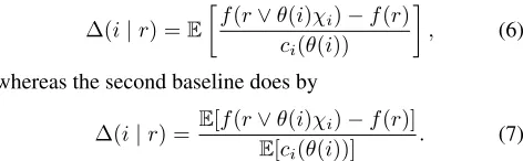
We compare these implementations with two baseline gorithms obtained by extending the well-known greedy al-gorithms for the maximization of set-submodular functions. The algorithms iteratively select an item that maximizes an evaluation metric defined as follows. Let S be the set of items chosen so far, andr∈[B]I be the realization vector (i.e,r(i) = 0fori∈I\S, andr(i)is the state ofifori∈S). Both of the algorithms evaluate an itemi∈I\Sby using the expected ratio of the function gain to the cost wheniis chosen. The first baseline evaluates the gain of itemiby
∆(i|r) =E
[f(r
∨θ(i)χi)−f(r)
ci(θ(i)) ]
, (6)
whereas the second baseline does by
∆(i|r) = E[f(r∨θ(i)χi)−f(r)]
E[ci(θ(i))]
. (7)
The details of these baseline algorithms are given in Algo-rithm 2.
We also incorporate a heuristic to pick items greedily into the implementations of the proposed algorithms; if all the budget is not spent after executing the rounding phase, the remaining items are picked greedily.
6.1
Recommendation
We first report the results on synthetic datasets constructed with a motivation to apply our algorithms to recommenda-tions. More concretely, we consider recommending items (e.g., news article or movie) to a user so as to maximize the user’s utility. If an itemiis recommended, then the user evaluates it through his/her action (e.g., skipping or reading articles). We defineBlevels of evaluations. The history of the recommendations is represented by a vectorr ∈ [B]I;
r(i) = 0indicates that item iis not recommended to the user, whereasr(i)>0means thatiis recommended to the user and its evaluation isr(i). When the evaluation for item
iisj, the user incurs a costci(j). Here, the cost is such as the fee or time to obtain the evaluationj. For example, in
pay-per-article news platforms, e.g., Blendle, the user needs to pay the fee for reading an article completely. We assume that the budgetCof the user is known or can be estimated from the user activities, and the task is to recommend items under the budget constraint defined byC.
We define the utility of the user by extending the prob-abilistic topic coverage function, that is often used in rec-ommendation (e.g., (El-Arini et al. 2009)). While the func-tion is originally defined as a set-funcfunc-tion, we extend it to an integer lattice for modeling the levels of evaluations. Let K be the number of topics. We define weight vec-tors w ∈ [0,1]K and φ
i ∈ [0,1]K (i ∈ I) such that ∑K
k=1w(k) = 1and
∑K
k=1φi(k) = 1for alli ∈ I.w(k) indicates a user’s preference for thekth topic, andφi(k) in-dicates the proportion of thekth topic in itemi. Givenwand
φi(i∈I), the utility functionf : [B]I →R+is defined by
f(r) = ∑
k∈Kw(k) (
1−∏ i∈I
(
1−r(i)φi(k) B
))
for each
r∈[B]I. This is monotone lattice-submodular.
In the experiments, we constructed probability distribution
pi: {1, . . . , B} →[0,1]randomly according to the symmet-ric Disymmet-richlet distribution with parameter1.0, and the vectors
wandφi(i∈I) were sampled from the symmetric Dirichlet distribution with parameterα. The costci(j)(i∈I,j ∈[B]) was set to⌈max{Cf(jχi),1}⌉. We considered 18 different settings corresponding to each combination of parameters
B ∈ {3,5},K∈ {5,15,30}, andα∈ {0.1,0.05,0.01}. In all experiments, bothCand|I|were set to 100. We gener-ated three datasets randomly from a single setting. For each dataset, the algorithms performed 100 random trials of adap-tive selection, and report the average of the objecadap-tive values attained by the algorithms.
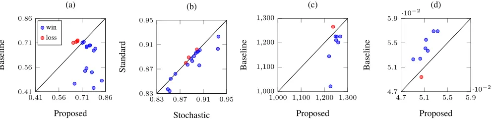
Figure 2 (a) compares the average objective values for 18 settings. In this figure, each point in the coordinate cor-responds to a single setting. The x-coordinate of a point shows the average objective value attained by the proposed algorithm with the stochastic continuous greedy algorithm, where the first baseline algorithm is used when the budget is not spent when the proposed algorithm terminates. The
y-coordinate represents the maximum of the average objec-tive values achieved by the two baseline algorithms. Hence, a point in the lower half indicates that the proposed algo-rithm outperformed both of the baseline algoalgo-rithms in the corresponding setting. We can observe that the proposed al-gorithm outperformed the baseline alal-gorithms in 14 settings. The difference between the objective values is large when the proposed algorithm is better, while the difference is small even when one of the baseline algorithms achieved a better objective value. This proves that the proposed algorithm is more stable than the baseline algorithms.
0.41 0.56 0.71 0.86 0.41
0.56 0.71 0.86
Proposed
Baseline
(a)
win loss
0.83 0.87 0.91 0.95 0.83
0.87 0.91 0.95
Stochastic
Standard
(b)
1,000 1,100 1,200 1,300 1,000
1,100 1,200 1,300
Proposed
Baseline
(c)
4.7 5.1 5.5 5.9 ·10−2
4.7 5.1 5.5 5.9·10
−2
Proposed
Baseline
(d)
Figure 2: Summaries of experimental results. A blue (red) point denotes our proposed algorithm was better (worse) than the compared baseline algorithms in the corresponding parameter setting.
6.2
Budgeted Batch-Mode Active Learning
Next, we report the results for applying the algorithms for CSSMP to a budgeted batch-mode active learning. In this problem, we have a setDof data, wherein each data point is represented by a feature vectorx∈Rdand is associated with a labely ∈ {−1,1}. However, the labels of data are not known in advance. The purpose is to select a part of the data to label under a budget constraint so as to maximize the performance of a classifier trained from the labeled data.
In particular, we consider the following setting. The dataset
Dis divided into data subsets Di (i ∈ I), and we seek to select several subsets. A subsetDi consists of data points
xi1, . . . , xiB. If subsetDiis selected, then the data points in
Diare processed sequentially fromxi1toxiB. It is unclear how many data points are processed in advance, but we know the probabilitypi(j)that the processing ofxi1, . . . , xij is completed but that ofxij+1is not. How many data points in Diwill be processed is revealed immediately after selecting
Di, and a costci(j)from the budget is paid if data points
xi1, . . . , xij will be processed. Each item in CSSMP corre-sponds to each subset, and the state of an item correcorre-sponds to the number of processed data points in the subset. We assume that at least one data point will be processed ifDiis selected. We consider algorithms to select subsets adaptively under the constraint that the total cost does not exceed budgetC.
To obtain a better classifier, we should maximize the informativeness of the processed data points. In order to measure informativeness, we use a function derived from the Fisher information ratio of logistic regression (Hoi et al. 2006). This function is defined from an existing linear classifier parameterized by a weight vectorβ ∈ Rd and a bias term β0 ∈ R. Define η: Rd → (0,1/4] asη(x) =
1 1+eβ⊤x+β0
(
1− 1 1+eβ⊤x+β0
)
. Letγbe a small positive
pa-rameter. Letr∈[B]I be the vector representing how many data points in each subset will be processed;r(i) =j >0
represents thatDi is selected and data pointsxi1, . . . , xij in Di are processed, whereas r(i) = 0 means that Di is not selected. Then, the objective function f: [B]I →
R+ is formulated by f(r) = γ1∑i∈I ∑B
j=1η(xij) − ∑
i∈I ∑
j>r(i)
η(xij)
γ+∑ i′ ∈I
∑r(i′)
j′=1η(xi′j′)(x⊤ijxi′j′)2
. The
mono-tonicity and the lattice-submodularity of this function fol-low from the monotonicity and submodularity of the set-function considered in Hoi et al. (2006).
For our experiments, we used the WDBC dataset (569 instances; 32 features) from the UCI machine learning repos-itory (http://archive.ics.uci.edu/ml). We used half of the dataset for the pooled data and the other for the test data. First, we randomly selected 20 initial instances from the pooled data and learned theL2-regularized logistic regression using
the initial data to obtainβ andβ0. Then, we selected addi-tional instances from the pooled dataset by using the baseline and proposed methods for CSSMP under a budget constraint. Notice that the given labels of these instances are not used up to this point. Finally, with the labels of these instances, we again learned the classifier by using the initial and additional instances.
To implement the logistic regression, we used scikit-learn (http://scikit-learn.org). For all training of the logistic re-gression, the regularization parameterρwas selected from
{0.1,0.5,1.0,2.0,10.0}by 5-fold cross-validation. All fea-tures in the dataset were standardized; it makes each feature have zero mean and unit variance. Note that we did not scale the features so that||x||2
2= 1for improving the performance
of the classifiers.
Candγwere set to 100 and 0.01 respectively.pi(i∈I) was constructed randomly according to the symmetric Dirich-let distribution with parameter1.0. To make the correlation between performance and costs, we sorted all the instances in the pool data by the objective function values, then di-vided the sorted instance list into the subsets. We considered eight experimental settings onBand item costs;Bwas se-lected from{3,4,5,6}, andci(j)(i∈I;j ∈[B]) was set to⌈max{Cf(jχi),1}⌉or⌈max{jCf(jχi)/B,1}⌉. In the same as the experiments of recommendation, we generated three datasets randomly from each setting, repeated the trial of selections 100 times, and report the average of the objec-tive values and the error rates attained by the algorithms.
point in the upper half indicates that the proposed algorithm is better than the baseline algorithms. It can be observed that the proposed algorithm reduced the error of the classifier in seven settings.
7
Conclusion
We considered adaptive algorithms for CSSMP. In design of our proposed algorithms, we extend the framework of the contention resolution scheme, known to be useful in the maximization problem of set-submodular functions, to lattice-submodular functions. We believe these contributions to be potentially useful in other problems related to lattice-submodular functions.
Through the experiments, we verified that algorithms out-put better solutions compared with baseline algorithms. A disadvantage of our algorithms is their computational com-plexity. In particular, the continuous optimization phase (re-lying on the continuous greedy or the stochastic continu-ous greedy algorithm) is slow. There are several attempts to speed up this part (Badanidiyuru and Vondr´ak 2014; Chekuri, Jayram, and Vondr´ak 2015), and it is a future work to consider them in our algorithms.
References
Adamczyk, M.; Sviridenko, M.; and Ward, J. 2016. Sub-modular stochastic probing on matroids. Mathematics of Operations Research41(3):1022–1038.
Ahmed, A.; Teo, C. H.; Vishwanathan, S. V. N.; and Smola, A. J. 2012. Fair and balanced: learning to present news stories. InProceedings of the Fifth International Conference on Web Search and Web Data Mining, 333–342.
Asadpour, A., and Nazerzadeh, H. 2016. Maximizing stochas-tic monotone submodular functions. Management Science
62(8):2374–2391.
Badanidiyuru, A., and Vondr´ak, J. 2014. Fast algorithms for maximizing submodular functions. InProceedings of the Twenty-Fifth Annual ACM-SIAM Symposium on Discrete Algorithms, 1497–1514.
C˘alinescu, G.; Chekuri, C.; P´al, M.; and Vondr´ak, J. 2011. Maximizing a monotone submodular function subject to a matroid constraint.SIAM Journal on Computing40(6):1740– 1766.
Chekuri, C.; Jayram, T. S.; and Vondr´ak, J. 2015. On multi-plicative weight updates for concave and submodular func-tion maximizafunc-tion. InProceedings of the 2015 Conference on Innovations in Theoretical Computer Science, 201–210. Chen, Y., and Krause, A. 2013. Near-optimal batch mode active learning and adaptive submodular optimization. In
Proceedings of the 30th International Conference on Machine Learning, 160–168.
El-Arini, K.; Veda, G.; Shahaf, D.; and Guestrin, C. 2009. Turning down the noise in the blogosphere. In Proceed-ings of the 15th ACM SIGKDD International Conference on Knowledge Discovery and Data Mining, 289–298.
Feldman, M.; Naor, J.; and Schwartz, R. 2011. A unified con-tinuous greedy algorithm for submodular maximization. In
IEEE 52nd Annual Symposium on Foundations of Computer Science, 570–579.
Feldman, M. 2013.Maximization Problems with Submodular Objective Functions. Ph.D. Dissertation, Technion – Israel Institute of Technology.
Fortuin, C. M.; Kasteleyn, P. W.; and Ginibre, J. 1971. Cor-relation inequalities on some partially ordered sets. Commu-nications in Mathematical Physics22(2):89–103.
Fujii, K., and Kashima, H. 2016. Budgeted stream-based active learning via adaptive submodular maximization. In
Advances in Neural Information Processing Systems 29, 514– 522.
Gabillon, V.; Kveton, B.; Wen, Z.; Eriksson, B.; and Muthukr-ishnan, S. 2013. Adaptive submodular maximization in ban-dit setting. InAdvances in Neural Information Processing Systems 26, 2697–2705.
Gabillon, V.; Kveton, B.; Wen, Z.; Eriksson, B.; and Muthukr-ishnan, S. 2014. Large-scale optimistic adaptive submodular-ity. InProceedings of the Twenty-Eighth AAAI Conference on Artificial Intelligence, 1816–1823.
Golovin, D., and Krause, A. 2011. Adaptive submodularity: Theory and applications in active learning and stochastic optimization. Journal of Artificial Intelligence Research
42:427–486.
Gotovos, A.; Karbasi, A.; and Krause, A. 2015. Non-monotone adaptive submodular maximization. In Proceed-ings of the Twenty-Fourth International Joint Conference on Artificial Intelligence, 1996–2003.
Gupta, A.; Krishnaswamy, R.; Molinaro, M.; and Ravi, R. 2011. Approximation algorithms for correlated knapsacks and non-martingale bandits. InIEEE 52nd Annual Sympo-sium on Foundations of Computer Science, 827–836. Gupta, A.; Nagarajan, V.; and Singla, S. 2017. Adaptivity gaps for stochastic probing: Submodular and XOS functions. In Proceedings of the Twenty-Eighth Annual ACM-SIAM Symposium on Discrete Algorithms, 1688–1702.
Hoi, S. C. H.; Jin, R.; Zhu, J.; and Lyu, M. R. 2006. Batch mode active learning and its application to medical image classification. InProceedings of the Twenty-Third Interna-tional Conference on Machine learning, 417–424.
Ma, W. 2014. Improvements and generalizations of stochastic knapsack and multi-armed bandit approximation algorithms: Extended abstract. InProceedings of the Twenty-Fifth Annual ACM-SIAM Symposium on Discrete Algorithms, 1154–1163. Yu, B.; Fang, M.; and Tao, D. 2016. Linear submodular bandits with a knapsack constraint. InProceedings of the Thirtieth AAAI Conference on Artificial Intelligence, 1380– 1386.