R E S E A R C H
Open Access
A framework for automatic heart sound analysis
without segmentation
Sumeth Yuenyong
1*, Akinori Nishihara
1, Waree Kongprawechnon
2, Kanokvate Tungpimolrut
3* Correspondence: toey123@gmail. com
1Department of Communication
and Integrated Systems, Tokyo Institute of Technology, Japan 2-12-1-W9-108 Ookayama, Meguro-ku, Tokyo, 152-8552 Japan Full list of author information is available at the end of the article
Abstract
Background:A new framework for heart sound analysis is proposed. One of the most difficult processes in heart sound analysis is segmentation, due to interference form murmurs.
Method:Equal number of cardiac cycles were extracted from heart sounds with different heart rates using information from envelopes of autocorrelation functions without the need to label individual fundamental heart sounds (FHS). The complete method consists of envelope detection, calculation of cardiac cycle lengths using auto-correlation of envelope signals, features extraction using discrete wavelet transform, principal component analysis, and classification using neural network bagging predictors.
Result:The proposed method was tested on a set of heart sounds obtained from several on-line databases and recorded with an electronic stethoscope. Geometric mean was used as performance index. Average classification performance using ten-fold cross-validation was 0.92 for noise free case, 0.90 under white noise with 10 dB signal-to-noise ratio (SNR), and 0.90 under impulse noise up to 0.3 s duration. Conclusion:The proposed method showed promising results and high noise robustness to a wide range of heart sounds. However, more tests are needed to address any bias that may have been introduced by different sources of heart sounds in the current training set, and to concretely validate the method. Further work include building a new training set recorded from actual patients, then further evaluate the method based on this new training set.
1 Background
Heart disease is a major health problem and a leading cause of fatality throughout the world. Treatment can be easier and cheaper if the condition is detected early. Cardiac disorders that are valve related can be detected efficiently and cheaply using ausculta-tion. Unfortunately, auscultation requires extensive training and experience to perform effectively, and such training has been on the decline due to the availability of new car-diac examination technologies [1]. Regardless, auscultation remains the most cost-effective method for cardiac examination because it requires minimal equipment. This makes auscultation the primary and often the only means of cardiac examination avail-able for small primary health care clinics. In reality, however, medical personnel in these clinics have little or no training in auscultation. The benefits of automatic auscul-tation can be considerable.
Auscultation consists of two phases: heart sound acquisition and heart sound analysis. Heart sound acquisition involves placing a stethoscope at the appropriate location on a patient’s chest with the right amount of force to capture heart sound. Heart sound ana-lysis is used to determine whether or not the captured sound corresponds to a healthy or diseased heart. This work is part of a larger study whose aim is to create a remote auscultation system, a robotic device that can perform both heart sound acquisition and analysis. Since acquisition is mostly a mechanical process, this work focuses only on the analysis. The work focuses further on only detecting the presence of a disorder, but does not attempt to identify it. That is, heart sounds are classified into two classes:“healthy” or“diseased”. While this is a simpler problem than the multi-class problems (providing diagnosis of the type of the disease) addressed by most studies on heart sound analysis, it allows for a method that does not require heart sound segmentation and thus, is robust to sounds that are difficult to segment due to significant signal corruption.
1.1 Heart Sounds and Cardiac Cycles
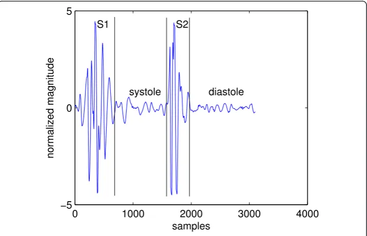
Heart sounds in healthy adults consist of two events: the first heart sound (S1) and the second heart sound (S2). Together they are referred to asfundamental heart sound(FHS). A cardiac cycle or a single heartbeat is defined as the interval between the beginning of S1 to the beginning of the next S1. The interval between the end of S1 to the beginning of the same cycle’s S2 is calledsystoleand the interval between the end of S2 to the begin-ning of the next cycle’s S1 is calleddiastole. In, general systole is shorter than diastole, which is the assumption that most heart sound segmentation methods are based on. Figure 1 shows a cardiac cycle with the components separated by black vertical lines.
1.2 Abnormal Heart Sounds
Cardiac cycles of abnormal heart sounds contain components that are not one of the FHS. These components can be grouped into two types: extra heart sounds and murmur sounds. An example of the first type is the third heart sound (S3) shown in Figure 2.
0 1000 2000 3000 4000
−5 0 5
normalized magnitude
samples S1
systole S2
diastole
The second type of abnormal heart sound is called a murmur. They are caused by turbu-lence blood flow through a blocked (stenosis) valve, or backward flow through a leaking (regurgitation) valve. These sounds can be heard both in systole or diastole, depending on the underlying condition. The presence of murmur is a good indicator of valvular (valve related) disorders. Figure 3 shows a cardiac cycle with a murmur called aortic regurgitation caused by leakage of the aortic valve. It can be seen by comparing Figure 2 and 3 that murmurs are fundamentally different from normal heart sounds. Whereas S3 looks like an extra copy of FHS, murmurs alter the waveform of a cardiac cycle comple-tely and the locations of FHS can no longer be marked precisely. This can cause pro-blems for heart sound analysis in the segmentation state because most segmentation
0 2000 4000 6000 8000
−8 −6 −4 −2 0 2 4 6 8
samples
normalized magnitude
S3 S2
S1 S1
Figure 2A cardiac cycle with third heart sound.
0 1000 2000 3000 4000
−6 −4 −2 0 2 4 6 8
samples
normalized magnitude
algorithms are based on determining the locations and types of FHS. It can be seen that abnormal heart sounds are characterized by the presence of extra components in their cardiac cycles that are not FHS. Thus one could formulate a heart sound analysis pro-blem as detection of components other than FHS in cardiac cycles.
1.3 Overview of Heart Sound Analysis
Heart sound analysis can be broken into three generic steps: segmentation, feature extraction, and classification. Segmentation is to determine the boundaries of cardiac cycles from contiguous heart sound signals. Feature extraction is to calculate the iden-tifying parameters from each cardiac cycle. classification is to make a decision on a heart sound’s type based on those parameters.
There are two approaches to segmentation: envelope based and machine learning based. Most existing algorithms use the envelope approach since it is not necessary to label different components of cardiac cycles manually. On the other hand, if labelled cardiac cycles are available, then a machine learning approach is preferred because tedious envelope analysis can be avoided. The details of segmentation is discussed next.
1.4 Segmentation
Segmentation has been the subject of many studies because it is the first and perhaps the most difficult step in heart sound analysis. The most popular approach to segmentation can be called the“envelope analysis”approach. This approach calculates the envelope signal of a heart sound, detects peaks of the envelope signal, establishes which peaks cor-respond to S1 and which corcor-respond to S2 and, then forms cardiac cycles using the S1-S1 intervals. Examples of this approach include [2], using average normalized Shannon energy, [3] using homomorphic filtering, [4] using complexity signatures, [5] using energy of wavelet coefficients and [6] comparing various envelope detection methods. All these studies fall under the envelope analysis approach since they are all based on analysis of the envelope signals and are different only by envelope detection methods. Due to its widespread use, the envelope analysis approach in general is discussed next. 1.4.1 Segmentation of Normal Heart Sounds
Figure 4 shows a plot of healthy heart sound and its envelope signal calculated using the homomorphic filtering method. Peaks in the envelope signal correspond to the FHS, which in healthy heart sound can all be easily detected by thresholding. The threshold is indicated by the horizontal line. A peak is defined as a segment of signal between two consecutive threshold crossings and its location is marked at the maxi-mum sample in the segment. Any group of three consecutive peaks is then analysed. The distance between the first and second peak (p1-p2 in Figure 4) is calculated and compared with the distance between the second and third peak (p2-p3). Based on the assumption that systole is shorter than diastole, it is easy to identify systole as the shorter interval; thus, S1 must be the peak to the left of systole, or equivalently, S2 must be to the right. The identify of just one peak allows all other peaks to be identi-fied by noting that S1 and S2 must alternate. Boundaries of cardiac cycles are then formed by the S1-S1 intervals and segmentation is completed.
1.4.2 Segmentation of Abnormal Heart Sounds
leftmost peaks are analysed, which actually correspond to S1, S2, and S3, respectively. The third peak is an extrapeak such that it does not correspond to any FHS. Due to the presence of this peak (marked as “extra peak” in Figure 5), the length of p2-p3 interval has changed. It is no longer the distance between the second and the fourth peak, like it should be without the extra third peak, but the distance between the sec-ond and third peak. This is shorter than the p1-p2 interval and leads to the false con-clusion that the second peak is S1. Using this peak as a reference to label all other peaks leads to wrong identification of all peaks in the envelope signal and ultimately wrong segmentation results.
Segmentation is even more difficult in the case of heart sound with murmur. Figure 6 shows a cardiac cycle with aortic regurgitation murmur and its envelope signal. Aortic
0 2000 4000 6000 8000 10000
−5 0 5
normalized magnitude
0 2000 4000 6000 8000 10000
0 0.5 1
samples
S2
p2−p3 p1−p2
S1 S2 S1 S2 S1
Figure 4Segmentation of normal heart sound.
0 2000 4000 6000 8000 10000
−5 0 5
normalized magnitude
0 2000 4000 6000 8000 10000
0 0.5 1
samples
S1 S2
S1 S2 S3
real p2−p3 false p2−p3 S1 p1−p2
regurgitation is characterized by diastolic murmur, in addition to diminished S1 sound [7]. From the figure it can be seen that just one cardiac cycle contains 4 peaks, the lar-gest of which corresponds to S2. However, there is no clear location of S1 as can be seen from the top panel, where S1 appears to have been“squashed”. Therefore the envelope signal has 3 peaks that can not be labelled because the location of S1 is uncertain. For this reason, segmentation using the envelope analysis approach needs to eliminate extra peaks while retaining the ones that correspond to FHS. This is called“peak condition-ing”. In general, peak conditioning is based on“minimum peak interval”. That is, if an interval between consecutive peaks fall below the minimum interval, it indicates that one of them must be an extra peak; and a common procedure is to eliminate the one with smaller magnitude. Peak conditioning can become a very tedious process due to several reasons:
1. Depending on where and how hard the stethoscope is placed on the chest, the FHS peaks may actually be smaller in magnitude than the extra peaks. Thus a threshold could be too high, so that one or more FHS are missed. This means that the missing FHS peaks must also be detected; if this is done by lowering the threshold, more extra peaks could be detected.
2. In cases with severe murmur, one of the FHS may become very large and the other may disappear from the envelope signal altogether.
3. The assumption that systole is shorter than diastole is not always true. The length of diastole decreases with increasing heart rate; above a certain heart rate it becomes roughly the same length as systole.
4. Some cardiac cycles may be incorrectly segmented and there is no way to auto-matically distinguish correctly segmented cycles from incorrectly segmented ones. Allowing incorrectly segmented cycles to enter feature extraction results in bad training vectors for the classifier.
0 1000 2000 3000 4000
−10 0 10
normalized magnitude
0 1000 2000 3000 4000
0 0.5 1
samples
Due to difficulties in the envelope analysis approach, segmentation methods based on machine learning such as hidden Markov models (HMM) or time-delayed neural net-work (TDNN) have been proposed [8,9]. Using these approaches, tedious envelope analysis can be avoided at a cost of having to prepare training data for the HMM or TDNN by manual segmentation. That is, a training set has to be hand-labelled by a human expert. In practice however, cardiologists often use the carotid pulse which can be felt in the neck artery during systole to aid in identifying the FHS. Therefore label-ling a heart sound by visual inspection of the waveform alone can be challenging even for an expert. It can be seen that segmentation is a difficult problem, but under the method proposed in this work, it is not necessary to identify the FHS. The only infor-mation needed is the auto-correlation of the envelope signal, which makes it applicable even for heart sound waveforms that have been heavily corrupted by extra components.
1.5 Feature Selection and Extraction
Feature sets found in the literature can roughly be grouped into two types. The first employs medical knowledge about specific diseases and how they affect the genera-tion of heart sounds. An example of a feature of this type is the split S2 interval. Many cardiac disorders cause S2 to split into two separate sounds. Other types of features are based on time-frequency signal representations. This type of representa-tion is particularly suitable for heart sounds since they are non-starepresenta-tionary signals whose frequency content changes with time. A particular time-frequency representa-tion commonly used in heart sound analysis is the discrete wavelet transform (DWT) [10]. Other types of time-frequency representations of heart sounds were studied in [11] and it was shown that DWT is the most suitable representation. DWT had been used repeatedly for features in heart sound analysis by dividing detail level 2 (d2) coefficients into non-overlapping portions, then, calculating the signal power of each to form elements of a feature vector [12-14]. DWT based fea-tures offer two advantages over the first approach. They are well-studied in signal processing and many software packages exist for their calculation. This makes them easier to implement, compared to ad-hoc features extraction. Moreover, DWT coeffi-cients are unaffected by the type of envelope detection method used, since they are calculated directly from heart sound signals.
1.6 Using the DWT for Heart Sound Segmentation
reconstruct the signal. However in this study it was found that this may not always be the case because:
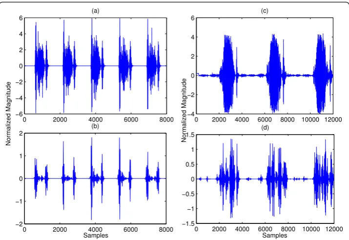
1. Often murmur can be eliminated by DWT decomposition and reconstruction. However, when a murmur is very loud, it overlaps with the FHS both in time and in frequency, and hence cannot be eliminated by the DWT method. Figure 7 com-pares the result of applying the DWT method described in [15] on a heart sound with moderate murmur and that with a very loud murmur. It can be seen in the left column that the murmur has been significantly removed. On the other hand, in the right column, the murmur is still largely present.
2. The extra heart sounds S3 and S4 are very similar to S1 and S2 in terms of fre-quency content. Therefore the DWT method cannot eliminate these sounds and their presence could compromise subsequence segmentation.
3. Some types of cardiac disorders can make S1 or S2 disappear altogether, such as severe aortic stenosis. Any segmentation algorithm based on locating the FHS would not work in this case.
For these reasons, it can be seen that DWT may not always work for heart sound seg-mentation in general. In fact, in the literature, there is no segseg-mentation algorithm which claims to work on all types and degree of severity of abnormal heart sounds. Thus in this work we proposed a method that does not require segmentation altogether.
2 Method
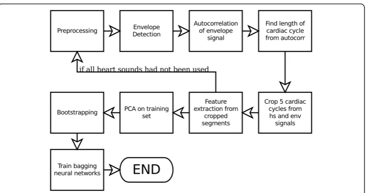
The heart sound analysis framework proposed in this work is shown in Figure 8. The main advantage of this approach is that it allows analysis to proceed without having to
0 2000 4000 6000 8000 −6 −4 −2 0 2 4 6
(a)
No rma l ized M agnitude
0 2000 4000 6000 8000 10000 12000 −4 −2 0 2 4 6 (c) No rma l ized M agnitude
0 2000 4000 6000 8000 −2 −1 0 1 2 (b)
Samples
0 2000 4000 6000 8000 10000 12000 −1.5 −1 −0.5 0 0.5 1 1.5
(d)
Samples
label each FHS. This is a big benefit for heart sounds with severe murmur whose FHSs are so corrupted that it becomes impossible to segment such sound. Obviously, such sound is abnormal, but in a traditional heart sound analysis approach that requires segmentation, it cannot be analysed, or could be miss-classified because of incorrect segmentation.
2.1 Preprocessing and Envelope Detection
Preprocessing consists of down-sampling and noise-removal of raw heart sound sig-nals. In this work a sampling frequency of 4000 Hz was used. Each sound in the train-ing set was either down-sampled or interpolated and re-sampled dependtrain-ing on its original sampling frequency. De-noising is based on DWT thresholding [17], with decomposition and thresholding parameters the same as that in [18].
Envelope signals were obtained from pre-processed heart sound signals by the fol-lowing equations, wherex denotes heart sound signals andEdenotes envelope signals [5]:
m
m
m
k k
a j k
( )1 4/ exp( ) exp( )
2 2
2 (1)
Y m n m k n x k
k N
( , ) ( ) ( )
1
(2)
E n Y m n m N
m M
( ) | ( , ) | , , , , .,
21
1 2 (3)
where ψm(k) defines the mother wavelet of a Complex Morlet wavelet with scale
parameter am. Equation 2 defines ascalogram, a 2-dimensional representation of a
sig-nal where one variable is time and another is scale. Yis a matrix whose rows corre-spond to scale and whose columns correcorre-spond to time. Equation 3 takes the magnitude of each element in Yand sums each column to get the envelope signal E.
The scale parametersamwere chosen such that they correspond to a frequency range
of 10 to 300 Hz, where the frequency bins are logarithmically spaced with 8 bins per octave. This means that the frequency range between 10 and 20 Hz was divided into 8 bins, and the frequency range between 20 and 40 Hz was also divided into 8 bins. This repeats until 300 Hz. The corresponding scales to these frequency bins were obtained by:
s F
F c
, (4)
whereFis the frequency,Fcis the center frequency of the mother wavelet, which is 5
rad/s for Complex Morlet wavelet, and Δis the sampling period. This approach to envelope detection has an advantage over other approaches such as those in [2,3]. Since the shape of Complex Morlet is very similar to that of an FHS, Ewill have high peaks where FHS occur and will be attenuated everywhere else.
2.2 Determine Lengths of Cardiac Cycles
Envelope signals were used to determine lengths of cardiac cycles by employing their autocorrelation [8,19],
R m x n m x n m
R m m
xx n
N m
xx
( ) ( ) ( ) ,
( )
01
0
0
(5)
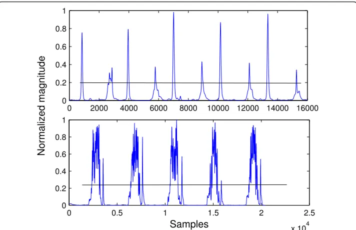
where Nis the signal length. Only positive values of m need to be considered since heart sound signals are real. The length of a cardiac cycle was determined by seeking for the first peak after the origin in the envelope of its autocorrelation function. Since heart sounds are nearly periodic signals, auto-correlation of envelope signals will have peaks where the shifted signal x(n+m) has been shifted by exactly one period and its cardiac cycles are aligned with those of the unshifted x(n). Figure 9 shows a heart sound signal in the top panel and the auto-correlation of its envelope signal in the bot-tom panel. The waveform in the botbot-tom panel was searched for a maximum within the domain of 1000 to 5000 samples from the beginning of the signal. Atfs= 4000 Hz this
domain corresponds to heart rates of 48 to 240 beats per minute (BPM), which account for usual human heart rates. The BPM information also allows for identifica-tion of abnormal heart rates. The peak marked by a circle is the maximum sample. It can be seen that the distance (number of samples) from this sample to the start of the signal is roughly the same as the length of the first cardiac cycle in the top panel. The assumption is that heart rate remains constant throughout the entire signal.
processing required. There is also a practical reason: short auscultation listening time which decreases the time it takes to examine a patient.
2.3 Feature Extraction
The feature set used in this work consists of two parts: three features come from the envelope segments and another 32 come from heart sound segments. Features were obtained from heart sound segments using the same method as in [12] where d2 DWT coefficients decomposed for six levels using Daubechies-2 wavelet were parti-tioned into 32 non-overlapping windows and the signal energy of each window was used as a feature. This procedure is illustrated in Figure 10. It yields a 32-element fea-ture vector for each heart sound segment. Another three feafea-tures were obtained from envelope segments. Figure 11 shows an envelope segment. Each peak is marked with a circle and a peak interval and is shown by the arrows. The features derived from it were: the number of peaks, the average distance (in samples) between consecutive peaks, and the signal energy of the whole segment. The peak detection algorithm used to obtain the first two of these features is an improvement over simple thresholding; its pseudo code is shown below.
M= blank 1 by 2 matrix
x= 1, 2, ..., length(E) {Eis envelope signal}
mx= -∞
mxpos= 0
fori= 1; length(E)do t= 1
ift>mxthen mx=t mxpos=x(i)
end if
ift<mx-Δthen
0 0.5 1 1.5 2
x 104 −5
0 5
0 0.5 1 1.5 2
x 104 0
500 1000
Normalized magnitude
Samples
M M
mxpos x {concatenate the row vector [mxpos x] vertically with matrixM}
end if end for
The difference between the above peak detection algorithm and simple thresholding can be seen by considering Figure 12 which shows a heart sound segment with severe aortic stenosis. If the threshold was set at around 0.25 as indicated by the black lines, simple thresholding would detect the same number of peaks as the number of thresh-old crossings divided by two; since there are many peaks above the threshthresh-old level, the result would be wrong. However, the peak detection algorithm used in this work would detect the correct number of peaks because in this case a peak is considered to be a maxima whose value is higher than the two “valleys” on either sides, by a thresh-old. That is, the threshold is compared from the top of a maxima, not from the x-axis.
Figure 10Feature extraction from heart sound segment.
0 0.5 1 1.5 2
x 104 0
0.1 0.2 0.3 0.4 0.5 0.6 0.7 0.8 0.9 1
Samples
Normalized magnitude
peak interval
Finally for the third feature, the sum of all samples in a segment were simply added. The 3-element vectors and 32-element vectors were concatenated, forming 35-element feature vectors.
2.4 Principal Component Analysis
Principal Component Analysis (PCA) is a linear transformation method. In this work the following form was used:
AQB, (6)
where AandBare matrices whose columns are feature vectors and Qis a matrix whose rows are eigenvectors of the covariance matrix of the training set C, arranged in decreasing order of magnitude of their eigenvalues from the top to bottom row. C is defined as:
C a a a a
1 1
1
n i i
T
i n
, (7)
wherenis the number of feature vectors,ai are the raw feature vectors, andā is the
mean vector. The use of PCA allows for a significant dimension reduction for the fea-ture vectors. This is because only eigenvectors whose sums of eigenvalues make up 90% of the sum of all eigenvalues are included in Q(the ones with larger eigenvalues were included first); and Cusually has many eigenvectors with small eigenvalues and few with large ones. The next pseudo code demonstrates the use of PCA on a raw fea-ture vector set, where the vectors are arranged as columns of matrixX.
C= 38 by 38 matrix of zeros
N= number of columns ofX
0 0.5 1 1.5 2 2.5 x 10⁴ 0
0.2 0.4 0.6 0.8 1
Samples
0 2000 4000 6000 8000 10000 12000 14000 16000 0
0.2 0.4 0.6 0.8 1
Normalized magnitude
fori= 1®Ndo
C C
xix
xix
Tend forC C
N 1
calculate eigenvalues and eigenvectors of C
Let E[v1T,,vTN] where each row ofEis an eigenvector and
Let D= [d1, ...,dN] their eigenvalues, wheredi≥di+1 S= sum ofD
k=Q= 0
whileQ≤0.9Sdo Q=Q+D(k)
k=k+ 1 end while
E =E(k+ 1, ...,N) (drop thek+ 1thtill Nthrows ofE) fori= 1®Ndo
yi=Exi(Eachyiis a new feature vector) end for
2.5 Bootstrapping and Bagging Classifiers
Let the original set of feature vectors and their class labels be denoted as T= {xi,di},
were xi is a feature vector and di its class label. After PCA, T was transformed into
T { , }xi di , where xi denotes feature vectors that have been transformed by PCA.
Bootstrapping is to randomly sample from T’ to generate N new training sets
T T1, 2,,TN, such that each is the same size asT . The sets Ti were training sets for
Nindividual neural networks (from here referred to as a network) which were trained independently using their respective training sets. During training, some members from each of the Ti were reserved for testing, that is, were excluded from training. Each network was trained, then, its performance was evaluated on the reserved test set. Then it was retrained and evaluated again for 30 times. The network instance that had the best performance was kept. This process was repeated Ntimes for all of the networks. Once all networks were trained they form “bagging classifiers”, which are multiple classifiers working together to classify an input. An unknown feature vector can be classified by taking the vote of the outputs of the networks by:
i L ni Y T
i
, 1
0 if
otherwise (8)
c n
N i
i N
1
2 0
1
if floor
otherwise
(9)
whereLis a set of all networks,Yithe output of a networki,nian intermediate
in [20] that the classification performance of bagging predictors is always equal to or greater than that of a single classifier. Therefore, unless limited by computational resources, bagging classifiers are preferred over a single classifier. An unknown heart sound to be classified would pass through all steps in Figure 8, up to and including PCA, using the transformation matrixQderived from the original training setT. The output of which becomes the input of all theNneural networks, and the decision of the heart sound type is made according to Equation 8 and 9.
In summary, the proposed heart sound analysis framework consists of:
1. Preprocessing that consists of down-sampling and noise-removal. 2. Envelope detection using Equation 1-3.
3. Calculate auto-correlation function of envelope signals.
4. Detect the location of the first peak in the domain of 1000 - 5000 samples after the origin of auto-correlation functions to find lengths of cardiac cycles.
5. Crop segments of five cardiac cycles from the heart sounds and the envelope signals.
6. Feature extraction from heart sound segments using DWT and from envelope segments using the peak detection algorithm in Section 2.3 to form 35-element fea-ture vectors.
7. Perform PCA on the feature vector setT using the second algorithm in Section 2.3.
8. Perform bootstrapping onT’to generateNtraining sets. 9. Train each network with its training set.
10. The trained networks classify heart sounds using Equation 8 and 9.
3 Results and Discussion
the classifier will not be biased toward the majority class [25]. Finally, the sounds came from different sources and thus were recorded with different equipment. This is a potential source of bias since the frequency response for each equipment are different. However this bias is potentially limited because there are more than two recording instruments, but only two classes. Thus, judging by the high classification performance, the classifier is not simply detecting the difference in frequency response. Such a sce-nario would have resulted in a much lower performance. Moreover, features based on envelope signal are insensitive to variations in frequency response, since frequency information has mostly been discarded during the envelope detection process. In con-clusion, due to these issues associated with the current training set, we would like to emphasize that this study is an initial evaluation of the proposed method. More experi-ments using real clinical sounds recorded with actual equipment, that will be used in the final auscultation device, are needed. This will be addressed in further work.
3.1 Evaluation Criterion
Ten-fold cross validation that incorporates bagging classifiers was used as performance evaluation; the flowchart of which is shown in Figure 13. It consists of dividing the data into ten portions. Then, in each fold, one portion was reserved for testing while the remaining nine became the training set, which was sampled according to the bootstrap-ping procedure discussed in section 2.5. This generatedNdifferent training sets for each of theNneural networks. The networks were trained and their performance was evalu-ated on the test portion, which is the same for all networks since the test portion was not sampled. Each network was trained 30 times and the instances that yielded the best performance were kept. This procedure is illustrated in Figure 13 inside the bounding boxes. Each box represents the training process of a single network. A network’s perfor-mance was evaluated by the sum of absolute error (SAE), defined in Equation 10:
SAE
|yi di|, i t(10)
where tis set of all instances of the test portion,yiis an actual output of a network
and diis the desired output (0 for normal and 1 for abnormal).
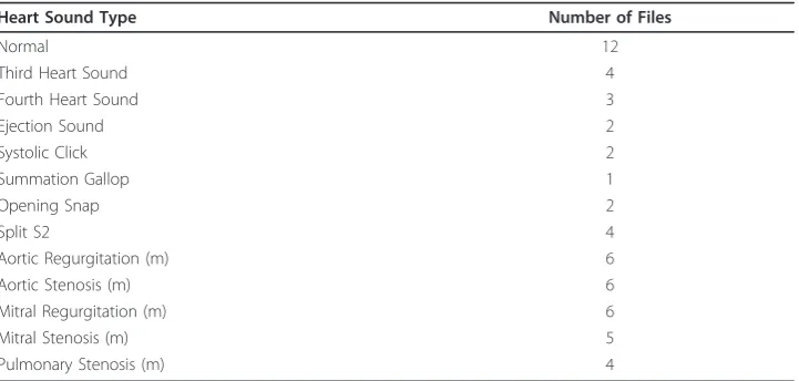
Table 1 Heart Sound Types in the Training Set
Heart Sound Type Number of Files
Normal 12
Third Heart Sound 4
Fourth Heart Sound 3
Ejection Sound 2
Systolic Click 2
Summation Gallop 1
Opening Snap 2
Split S2 4
Aortic Regurgitation (m) 6
Aortic Stenosis (m) 6
Mitral Regurgitation (m) 6
Mitral Stenosis (m) 5
Pulmonary Stenosis (m) 4
After the best Nnetworks had been obtained, each of them classified the test por-tion. The outputs that were higher than the thresholdT were rounded to one, while those that were not were rounded to zero. If the number of ones for a heart sound
were more than floor(N)
2 where Nis the number of networks, then that heart sound
was classified as abnormal. After all heart sounds in the test portion had been classi-fied, a different portion was selected as test portion and the whole procedure was repeated until all portions had been a test portion.
The reason why the networks had to be trained 30 times was because a network’s performance depends on its initial random weights, which determined the starting point on the error function. The error function of a neural network is generally not convex. Thus, the steepest descent may get caught in a local minimum during the training process and hence the need to repeat training many times and keep the best performing network.
Cross-validation results can be quantified by 4 numbers: true positive (TP), false positive (FP), true negative (TN), and false negative (FN),
•TP: the ratio between samples which are actually positive over the number of samples classified as positive.
!
"# $
$
%&
"#
"# ' "#
!
(
) !
$*
"# $ $
%&
"#
"# ' "#
!
(
) !
$*
•FP: the ratio between samples which are actually negative over the number of samples classified as positive.
•TN: the ratio between samples which are actually negative over the number of samples classified as negative.
•FN: the ratio between samples which are actually positive over the number of samples classified as negative.
where positive means diseased heart sounds and negative mean healthy heart sounds. From these raw scores, 3 more indicators of performance can be calculated by:
accuracy TPTN
N (11)
sensitivity TP
TP FN
(12)
specificity TN
TN FP
(13)
where Nis the number of samples in the training set. Finally, a single indicator of classification performance combines both the sensitivity and specificity into a single quantity called the geometric mean [25]. This quantity was used to assess performance in all experiments.
g sensitivityspecificity (14)
3.2 Experiment 1A - Determining the Optimal Number of Hidden Neurons
The purpose of experiment 1A was to determine the optimal parameters for the classi-fier which can be used for later experiments. Only a single neural network was used, with decision threshold T fixed at 0.5. Its classification performance was tested with increasing number of hidden neurons until there is no increase in performance. This was performed three times and the average was taken. The result is shown in Table 2. There was only a slight performance increase when the number of hidden neurons was increased from 5 to 10. Thus the experiment was stopped and 10 was chosen to be the optimal number of hidden neurons, which was fixed for all later experiments. The receiver operating characteristic (ROC) curve in Figure 14 was plotted to determine the best value for the threshold T , where the optimal point on the ROC curve is marked with a circle. The corresponding threshold value was around T= 0.15 and this value was used as the decision threshold for all later experiments. Also, from experi-ment 2A onward, bagging predictors with five networks was used. In summary, the optimal parameters determined by experiment 1A are 10 hidden neurons and T= 0.15.
3.3 Experiment 2A - Robustness to White Noise Test
SNR of 15 dB and 10 dB, there was little difference from the noise-free case. However, at 5 dB the performance noticeably decreased. This test showed that the system has some robustness to white noise, but in actual operation, loud background noise is something to be careful of.
3.4 Experiment 2B - Robustness to Impulse Noise Test
In actual operation of the system in a hospital, it may encounter impulse-like noise. It is likely that the patient may move during recording, causing impulse-like noise in the recorded heart sound due to friction between the stethoscope’s chest-piece and the patient’s chest. In this experiment the robustness of the system against impulse-like noise was tested. A total of 16 sounds of both normal and abnormal type had impulse noise of various duration (0.1, 0.2 and 0.3 s) added by replacing a segment of a signal with random sequence with range {-max max} where max is the maximum value of Table 2 Result of Experiment 1A
Hidden neurons trial 1 trial 2 trial average
1 0.89 0.86 0.89 0.88
5 0.91 0.90 0.92 0.91
10 0.92 0.94 0.91 0.92
Cross validation result using only a single neural network and varying the number of hidden neurons. All performance values in this and all subsequence tables are given in the geometric mean defined in Equation 14.
that signal. Cross-validation was performed with these sounds mixed in the training set. The result is shown in Table 4. Impulse noise of all durations had little affect on the system’s performance. In practice, impulse noises are generally less than 0.3 sec-onds long so the system can be considered robust to impulse noise.
3.5 Experiment 2C - Robustness to Unseen Abnormal Heart Sound Types
In this experiment the goal was to assess the robustness of the system to abnormal heart sound types that were not part of the training set. Different abnormal sound types were left out of the training process and were used to test the system trained on the remaining sounds. The result is shown in Table 5. It can be seen that in most cases the left-out sounds have been correctly classified.
3.6 Discussion and Comparison with Other Works
The goal of this work is to provide a heart sound analysis algorithm for an automatic auscultation device. Such device will be used mostly in rural clinics as an early and cheap detection for heart disease, not as a main diagnosis device. This is the main rea-son why we decided to restrict the problem to be two-classes, and focus on incorporat-ing as many type of abnormal sounds as possible, and to be robust to noise.
From the experiments, it can be seen that the proposed method achieved average performance of 0.92 (all performance numbers are geometric means unless stated otherwise) for the noise-free case and 0.9 under additive white noise of 10 dB. This provides quite a comfortable noise margin, especially in rural clinics that tend to be noisy. In the extreme case where the noise level was increased to 5 dB, classification performance was significantly decreased to 0.83. A separate examination area, with the auscultation device placed as far away as space permits from any noise sources such as air conditioning, should be able to provide an SNR level within the robust range.
In actual auscultation, a patient may move slightly during recording. Such movement causes impulse noise which may affect the classification result. Experiment 2B showed that impulse noise up to 0.3 second in duration may be tolerated with only slight decrease in accuracy. Based on these results it can be concluded that if the SNR is kept higher than 10 dB and long impulse noise is relatively rare; one could expect around 0.90 classification performance from the proposed method.
The final experiment showed how the proposed method can be generalized to clas-sify abnormal sound types that were not part of the training set. In practice such cases Table 3 Result of Experiment 2A
SNR trial 1 trial 2 trial 3 average
15 dB 0.92 0.93 0.93 0.93
10 dB 0.88 0.91 0.91 0.90
5 dB 0.86 0.81 0.82 0.83
Cross validation result where the training set had white noise added at different SNR’s.
Table 4 Result of Experiment 2B
Noise duration trial 1 trial 2 trial 3 average
0.1 s 0.92 0.92 0.90 0.91
0.2 s 0.90 0.89 0.92 0.90
0.3 s 0.91 0.90 0.89 0.90
should be rare since the system must be trained extensively before being fielded, but it provides some confidence knowing that the algorithm is likely to generalize correctly if such a case does occur. Even split S2, which is hard to detect, was mostly classified correctly under ideal noise-free conditions.
It is difficult to make direct comparison between this work and others, because the goals are different, and there is no standard test set upon which to compare. Therefore, we dis-cuss some general comments on how the proposed method compares with other works in this field. In terms of classification accuracy alone, this method was not the best. Several studies reported over 98% classification accuracy. This makes our method seem inferior, especially when the focus is only on two-class situations, while many studies are multi-class, and identified the disease that a heart sound is showing. Our method however, has a wide coverage. There were 12 different types of abnormal heart sound in the training set, which is more than most other studies that often include only the four main types of mur-mur: aortic regurgitation/stenosis and mital regurgitation/stenosis. A diverse training set that includes abnormal sounds that are very similar to normal (split S2, small S3 and S4), makes accurate classification quite difficult even for the two-class case. The training set also included sounds such as that in Figures 3 and 7 that are very difficult to segment automatically, due to very large murmur and/or diminished FHS. In such situations the proposed method is highly advantageous since segmentation is not required, which is the unique point of this algorithm. The only“segmentation”performed is cropping out seg-ments of heart sound signals and their envelopes with lengths equal to 5 cardiac cycles of each respective sound. These segments can begin and end anywhere within a cardiac cycle, that is, the beginning of the segments do not have to align with the beginning of a cardiac cycle. This means that classification accuracy will not be affected by erogenous fea-ture vectors produced by miss-segmented cycles.
Robustness against noise is another main advantage of the proposed method, as indi-cated by the result of experiment 2A and 2B. Extracting multiple cardiac cycles to form a feature vector averages out the effect of any peculiarity in a particular cycle, such as impulse noise. Focusing only on two classes and skipping segmentation make the proposed method seem overly simple, but it allowed for high robustness and cover-age while not compromising practical use. This is because even if a patient has been diagnosed with a particular disease by heart sound analysis and referred to a hospital, Table 5 Result of Experiment 2C
Unseen type Accuracy
AR 4/5
AS 5/6
MR 5/5
MS 4/4
PS 3/3
S3 4/4
S4 3/3
Split S2 3/4
Ejection Sounds 2/2
Systolic Click 2/2
Opening Snap 2/2
then the patient will most likely be re-examined using techniques other than ausculta-tion before the condiausculta-tion is confirmed. Thus the proposed method is suitable for its intended use.
On the negative side, the training set used may have introduced bias, since sounds came from different sources and the normal set was over-sampled. Moreover, most sounds in the training set were recorded for instruction purpose so they are likely to be of better quality than actual clinical recordings. These issues will be addressed in further research by building a new training set using the same equipment, and recorded in the same environment where the final automatic auscultation device will be deployed. The method will be evaluated again using this new training set.
4 Conclusions
A new approach to heart sound analysis was proposed that does not require segmenta-tion. The method is applicable to a wide range of heart sounds, from normal to those containing severe murmurs where one of the FHS may disappear. The training set incorporated 12 different types of abnormal heart sounds ranging from split S2 to severe murmurs. Using geometric mean as index of performance and ten-fold cross validation, experiments were conducted to verify the effectiveness of the proposed method and to determine the optimal configuration for the classifier. Based on these parameters, further tests were conducted to assess the robustness of the system to white noise, impulse noise, and unseen heart sound types. The experiments showed that the system can operate at 10 dB SNR, and with 0.3 s long impulse noise with average performance of 0.9. In conclusion, the advantages of this work are:
1. It does not require segmentation.
2. It is applicable to a wide range of heart sounds. 3. It is robust to noise.
While the shortcomings of this work are:
1. It only classifies heart sounds as normal or abnormal.
2. The training set may have introduced bias due to different frequency response and oversampling of the normal set.
4.1 Further Work
Further works include stand-alone software implementation and field testing in a hos-pital using a new training set to concretely validate the proposed method. Also another approach based on single-class classification (SCC) may be explored. In SCC the train-ing data consists of samples from only a strain-ingle class, which is usually the “normal” class. Applying SCC to heart sound analysis reformulates the problem to be detection of healthy heart sounds and the classifiers would be trained using only healthy samples. This approach eliminates the need to collect abnormal samples and would make data collection much easier.
Acknowledgements
Neilson, an English instructor at SIIT, for proofreading this paper. This work was supported by the National Research University Project of Thailand Office of Higher Education Commission.
Author details 1
Department of Communication and Integrated Systems, Tokyo Institute of Technology, Japan 2-12-1-W9-108 Ookayama, Meguro-ku, Tokyo, 152-8552 Japan.2Department of Information, Computer and Communication Technology, Sirindhorn International Institute of Technology (SIIT), Thammasat University, Thailand 131 Moo 5, Tiwanont Road, Bangkadi, Muang, Pathum Thani 12000, Thailand.3Industrial Control and Automation Laboratory, National Electronic and Computer Technology Center (NECTEC), Thailand 112 Paholyothin Rd., Khlong Neung, Khlong Luang, Pathum Thani 12120, Thailand.
Authors’contributions
KT conceived of the study, procured the equipment and collaboration from Thammasat University hospital, and is the project leader. WK suggested ideas for features, edited the manuscript and provided some samples. AN outlined the envelope detection module and tested the code. SY coded the algorithm, conducted the experiments, and drafted the manuscript. All authors read and approved the final manuscript.
Competing interests
The authors declare that they have no competing interests.
Received: 19 August 2010 Accepted: 9 February 2011 Published: 9 February 2011 References
1. Syed Z, Leed D, Curthis D, Nesta F, Levin RA, Guttag J:A Framework for the Analysis of Acoustical Cardiac Signals. IEEE Transactions on Biomedical Engineering2007,1(51):651-662.
2. Liang H, Lukkarinen S, Hartimo I:Heart Sound Segmentation Algorithm Based on Heart Sound Envelograms. Computers in Biology1997,24:105-108.
3. Gupta CN, Palaniappan R, Swaminathan S, Krishnan SM:Neural Network Classification of Homomorphic Segmented Heart Sound.Applied Soft Computing2007,7:286-297.
4. Kumar D, Carvalho P, Antunes M, Henriques J, e Melo AS, Habetha J:Heart Murmur Recognition and Segmentation by Complexity Signatures.In Proceedings of the 30th IEEE EMBS Annual Conference2008.
5. Rajan S, Budd E, Stevenson M, Doraiswami R:Unsupervised and Uncued Segmentation of the Fundamental Heart Sounds in Phonocardiograms Using a Time-Scale Representation.In Proceedings of the 30th IEEE EMBS Annual Conference2006.
6. Choi S, Jiang Z:Comparison of Envelope Extraction Algorithms for Cardiac Sound Signal Segmentation.Expert Systems with Applications2008,13:1056-1069.
7. Poole-Wilson P, Walsh RA, O’Rourke A, Fuster V:Hurst’s The HeartMcGraw-Hill; 2000.
8. Schmidt S, Toft E, Gra C, Struijk J:Segmentation of Heart Sound Recordings from an Electronic Stethoscope by a Duration Dependent Hidden Markov Model.Computers in Cardiology2008,35:345-359.
9. Oskiper T, Watrous R:Detection of the First Heart Sound using Time-Delayed Neural Network.Computers in Cardiology2002,29:537-540.
10. Mallat S:A Wavelet Tour of Signal ProcessingBurlington MA: Academic Press; 1998.
11. Debbal S, Bereksi-Reguig F:Computerized Heart Sound Analysis.Computers in Biology and Medicine2006,38:263-280. 12. Olmez T, Dokur Z:Classification of Heart Sounds Using Artificial Neural Network.Pattern Recognition Letters2003,
24:617-629.
13. Ari S, Saha G:In Search of an Optimization Technique for Artificial Neural Network to Classify Abnormal Heart Sounds.Applied Soft Computing2009,9:330-340.
14. Reed TR, Reed NE, Fritzson P:Heart Sound Analysis for Symptom Detection and Computer-Aided Diagnosis. Simulation Modeling Practice and Theory2004,12:129-146.
15. S O, M T:A Heart Sound Segmentation and Feature Extraction Algorithm Using Wavelets.Proceeding of the First International Symposium on Control, Communication and Signal Processing2004, 235-238.
16. Chebil J, Al-Nabulsi J:Classification of Heart Sound Signals Using Discrete Wavelet Analysis.International Journal of Soft Computing2007,2:37-41.
17. Donoho DL:De-Noising by Soft-Thresholding.IEEE Transactions on Information Theory1995,4(3):613-627. 18. Messer SR, Agzarian J, Abbott D:Optimum Wavelet Denoising for Phonocardiograms.Microelectronics2001,32:
931-941.
19. Kumar D, Carvalho P, Antunes M, Henriques J:Noise Detection During Heart Sound Recording.Proceeding of the 31st Annual International Conference of the IEEE EMBS.
20. L B:Bagging Predictors.Machine Learning1996,26:123-140.
21. Heart Sounds and Murmurs.[http://www.dundee.ac.uk/medther/Cardiology/hsmur.html]. 22. Heart Sounds and Murmurs.[http://www.texasheart.org/Education/CME/index.cfm]. 23. Human Heart Sounds.[http://int-prop.lf2.cuni.cz/heart_sounds/h12/index.html]. 24. Virtual Stethoscope.[http://sprojects.mmi.mcgill.ca/mvs/mvsteth.htm].
25. Kubat M, Matwin S:Addressing the Curse of Imbalanced Training Sets: One-Sided Selection.Proceedings of the 14th International Conference on Machine Learning1997, 179-186.
doi:10.1186/1475-925X-10-13
Cite this article as:Yuenyonget al.:A framework for automatic heart sound analysis without segmentation.