Estimating temporal and spatial variation of ocean surface CO 2in the North Pacific using a self-organizing map neural network technique

www.biogeosciences.net/10/6093/2013/ doi:10.5194/bg-10-6093-2013

© Author(s) 2013. CC Attribution 3.0 License.

Biogeosciences

Estimating temporal and spatial variation of ocean surface

p

CO

2

in

the North Pacific using a self-organizing map neural network

technique

S. Nakaoka1, M. Telszewski1,*, Y. Nojiri1, S. Yasunaka1, C. Miyazaki1,**, H. Mukai1, and N. Usui2

1_{National Institute for Environmental Studies, 16-2 Onogawa, Tsukuba, Ibaraki 305-8506, Japan} 2_{Meteorological Research Institute, 1-1 Nagamine, Tsukuba, Ibaraki 305-0052, Japan}

*_{now at: International Ocean Carbon Coordination Project, Institute of Oceanology of Polish Academy of Sciences, Ul.} Powsta´nców Warszawy 55, 81-712 Sopot, Poland

**_{now at: Hokkaido University, Kita 8 Nishi 5, Kita-ku, Sapporo, Hokkaido 060-0810, Japan} Correspondence to: S. Nakaoka ([email protected])

Received: 4 February 2013 – Published in Biogeosciences Discuss.: 8 March 2013 Revised: 25 June 2013 – Accepted: 9 August 2013 – Published: 26 September 2013

Abstract. This study uses a neural network technique to

pro-duce maps of the partial pressure of oceanic carbon dioxide (pCOsea₂ ) in the North Pacific on a 0.25◦latitude×0.25◦ lon-gitude grid from 2002 to 2008. ThepCOsea₂ distribution was computed using a self-organizing map (SOM) originally uti-lized to map thepCOsea₂ in the North Atlantic. Four proxy parameters – sea surface temperature (SST), mixed layer depth, chlorophyll a concentration, and sea surface salin-ity (SSS) – are used during the training phase to enable the network to resolve the nonlinear relationships between the pCOsea₂ distribution and biogeochemistry of the basin. The observedpCOsea₂ data were obtained from an extensive dataset generated by the volunteer observation ship program operated by the National Institute for Environmental Stud-ies (NIES). The reconstructed pCOsea₂ values agreed well with thepCOsea₂ measurements, with the root-mean-square error ranging from 17.6 µatm (for the NIES dataset used in the SOM) to 20.2 µatm (for independent dataset). We con-firmed that thepCOsea₂ estimates could be improved by in-cluding SSS as one of the training parameters and by taking into account secular increases ofpCOsea₂ that have tracked increases in atmospheric CO2. EstimatedpCOsea₂ values ac-curately reproducedpCOsea₂ data at several time series loca-tions in the North Pacific. The distribuloca-tions ofpCOsea₂ re-vealed by 7 yr averaged monthlypCOsea₂ maps were similar to Lamont-Doherty Earth ObservatorypCOsea₂ climatology, allowing, however, for a more detailed analysis of

biogeo-chemical conditions. The distributions ofpCOsea₂ anomalies over the North Pacific during the winter clearly showed re-gional contrasts between El Niño and La Niña years related to changes of SST and vertical mixing.

1 Introduction

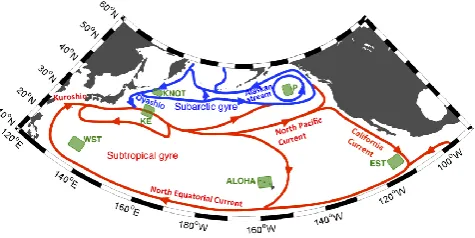
Fig. 1. Schematic map of the current system in the North

Pa-cific rewritten from Schmitz (1996) with the areas of three ocean time-series stations and three areas for comparison of seasonal and interannual variations ofpCOsea₂ and related oceanic parameters. “KNOT”, “P”, and “ALOHA” denote ocean time-series station areas in the North Pacific, and “WST”, “KE”, and “EST” denote ocean areas of the western subtropics, Kuroshio Extension, and eastern subtropics, respectively.

and estimated the annual global air–sea CO2 exchange at

−1.6±0.9 PgC yr−1.

Neural network (NN) techniques can be generally de-scribed as empirical statistical tools that resolve, to a certain degree, the nonlinear and often discontinuous relationships among proxy parameters without any a priori assumptions. In the past decade a handful of authors have reported the ap-plication of an NN technique to basin-scalepCOsea₂ analy-sis (e.g., Lefèvre et al, 2005; Jamet et al., 2007; Friedrich and Oschlies, 2009a, b; Telszewski et al., 2009), concentrat-ing mainly on the North Atlantic Ocean. Most recently, Tel-szewski et al. (2009) successfully applied a self-organizing-map (SOM) based NN technique to reconstructpCOsea₂ dis-tribution in the North Atlantic (10.5 to 75.5◦N, 9.5◦E to 75.5◦W) for three years (2004 to 2006) by examining non-linear/discontinuous relationship betweenpCOsea₂ and ocean parameters of sea surface temperature (SST), mixed layer depth (MLD), and chlorophylla concentration (CHL). One of the main benefits of this approach over the more traditional techniques, such as multiple linear regression (MLR), is that there are numerous empirical relationships established (e.g., 2220 in Telszewski et al., 2009) between examined parame-ters, allowing for more accurate representation of the highly variable system of interconnected water properties.

The North Pacific is dominated by two major current regimes: the subarctic and subtropical gyres (Fig. 1). The cold Oyashio Current and the warm Kuroshio Current are the western boundary currents of the North Pacific subarctic and subtropical gyres, respectively. The two currents meet at midlatitudes in the western North Pacific and turn to-ward the east as the North Pacific Current. The North Pa-cific has been typically characterized as a high-nutrient, low-chlorophyll region of the ocean at most of high latitudes be-cause of the low influx of iron to the ocean surface (Dugdale

and Wilkerson, 1991), and as a low-nutrient, low-chlorophyll region at the western and central low latitudes (Karl and Letelier, 2008; Lin et al., 2011). The Bering Sea, which is a marginal sea of the North Pacific, and coastal regions are upwelling areas within which the transport of nutrient- and CO2-rich subsurface water to the surface assures high bi-ological productivity (Chierici et al., 2006). In the North Pacific, there are expected to be thus quite large temporal and spatial variations ofpCOsea₂ . Zeng et al. (2002) reported that large temporal amplitude of1pCO2(pCOsea₂ –pCOair₂ ) over 60 µatm was apparent in the western-central subarc-tic and the eastern subtropics based on their measurements between 1995 and 1999.

For analysis of temporal variability ofpCOsea₂ or1pCO2 in the North Pacific, Stephens et al. (1995) estimated basin-scale monthly1pCO2distributions using simple linear re-gression analysis between pCOsea₂ and SST in 1985. Re-cently, Sarma et al. (2006) used MLR analysis to estimate pCOsea₂ from SST and satellite-based CHL observations in high-latitude regions of the eastern and western North Pa-cific, but the applicability of the MLR equations was limited to spring and summer. Takamura et al. (2010) also used MLR analysis to reconstructpCOsea₂ distributions as a function of SST and sea surface salinity (SSS) from 1999 to 2006 in mid-latitudes (25 to 40◦N, 120 to 150◦W, 140 to 170◦E).

The precise time-series analyses of pelagic oceanpCOsea₂ variability are limited to time-series stations (Bates, 2007, 2012; Dore et al., 2009; González-Dávila et al., 2010) where monthly pCOsea₂ observations are available over extended time periods. Two areas of frequent shipboard observations ofpCOsea₂ other than time-series stations are the eastern and western equatorial Pacific (e.g., Feely et al., 2006; Ishii et al., 2009), where the observed interannual pCOsea₂ varia-tions are associated with the El Niño–Southern Oscillation (ENSO). Another place where there have been frequent ship-boardpCOsea₂ observations in the North Pacific is the 137◦E repeat line (Midorikawa et al., 2006), where a weak but sig-nificant relationship between pCOsea₂ and ENSO has been observed. A basin-wide analysis of observedpCOsea₂ vari-ability (including the analysis of the interannual signal) has not yet been successfully performed. An atmospheric CO2 inverse model (Patra et al., 2005) and an ocean biogeochem-ical model (Valsala et al., 2012), however, suggest the possi-ble correlation of thepCOsea₂ variability with Pacific Decadal Oscillation (PDO).

Pacific (Fig. 1). We also presented the change of thepCOsea₂ distribution in response to the ENSO events.

2 Method and datasets

2.1 Method ofpCOsea₂ estimation

The study area includes the North Pacific from 10 to 60◦N and from 120◦E to 90◦W, and is hereafter called the North Pacific, although we have excluded coastal (bathymetric depth<500 m) and ice-covered (SST<−1.8◦C) areas from the analysis. In this study, we hypothesized that pCOsea₂ could be estimated by a linear function of time and an SOM function (fSOM)of four independent variables: SST, MLD, CHL, and SSS. The equation forpCOsea₂ then takes the following form:

pCOsea₂ =a×(t−tref)+fSOM(SST, MLD, CHL, SSS). (1) In Eq. (1)a is the secular rate of change of atmospheric CO2in µatm day−1,tdenotes the date, and the reference date trefis set to 30 June 2005. In addition, we assumedpCOsea₂ to be a linear function of time in order to take into account the influence of anthropogenic CO2emissions onpCOsea₂ , an effect that could not be accounted for by SST, MLD, CHL, or SSS. The anthropogenic influence onpCOsea₂ is consid-ered negligible for relatively short analyses, e.g., three years (cf., Lefèvre et al., 2005; Telszewski et al., 2009), but it builds up to around 10 µatm after seven years. Midorikawa et al. (2006) reported that the secular trend ofpCOsea₂ var-ied from 1.3 to 1.8 µatm yr−1_{(close to the rate of increase of} atmospheric CO2)in the western subtropical North Pacific based on their measurements over 20 yr along 137◦_{E. Wong} et al. (2010) also reported that their 30 yr time series of mea-surements along Line P, the line connecting ocean station P (50◦N, 145◦W) to the coast, showed that the long-term trend of pCOsea₂ tracked the increase of atmospheric CO2 in the eastern subarctic region. Takahashi et al. (2006) con-cluded that, for the most part, the increase of oceanic CO2in the North Pacific followed the increase of atmospheric CO2 for the last 35 yr with the increase rate varying geographi-cally, reflecting differences in local oceanographic biogeo-physical processes. We assumed in this study that the secular trend of pCOsea₂ was approximately a constant fraction of the rate of change of atmospheric CO2 over the North Pa-cific. Specifically, we assumed the value of the coefficienta in Eq. (1) to be 4.82×10−3 _{(=1.76/365.285) µatm day}−1_, which is the rate of increase of atmospheric CO2 concentra-tion converted from the CO2mole fractions (xCOair₂ )in the GLOBALVIEW-CO2 dataset (GLOBALVIEW-CO2, 2011) for the North Pacific region during the period of analysis.

The method for reconstructing pCOsea₂ is based on the methodology of Telszewski et al. (2009), but we allocated about three times as many neurons on a flat sheet map (53×115) to improve the estimate. A neuron in this study

is a vector that has four components: SST, MLD, CHL, and SSS. The values of these components, the training dataset, are prospectively normalized linearly (SST, SSS) or logarith-mically (MLD, CHL) to create an even distribution among the input variables (cf., Fig. 3 of Telszewski et al., 2009). As indicated schematically in Fig. 2, three processes are ex-ecuted in order to estimate basin-widepCOsea₂ fields in the SOM analysis procedure.

First, a neuron’s weight vectors (xi), which are linearly initialized, are repeatedly trained by input vectors (yj), by being presented with the normalized SST, MLD, CHL, and SSS values, until the statistical composition of the training dataset is extracted and the neural network sufficiently rep-resents the nonlinear interdependence of proxy parameters used in training (Training Process in Fig. 2a). At each step, Euclidean distances (D) are calculated between the weight vectors of neurons and the input vector:

D xi,yj

=

h

xi_SST−yj_SST

2

+ xi_MLD−yj_MLD

2

+ xi_CHL−yj_CHL

2

+ xi_SSS−yj_SSS

2i0.5. (2)

The neuron closest to the training data point in Euclidean distance terms, here called the winner, is adjusted towards its value by a fraction of this distance dictated by the linearly time-decreasing learning function. At the same time, the neu-rons in the vicinity of the winner are also adjusted towards the value of the training data point by a fraction of the win-ner’s adjustment in accordance with a time-decreasing Gaus-sian function, as explained by Kohonen (2001). This process results in clustering of similar neurons and self-organization of the map. The observedpCOsea₂ dataset is not required at this stage of the analysis.

Second, each neuron is labeled with an observedpCOsea₂ value. Technically, the labeling process follows the same principles as the training process. The labeling data, which in this study consist of the observedpCOsea₂ value assigned to a reference year by adding/subtracting the assumed tem-poral change ofpCOsea₂ and coincided with normalized SST, MLD, CHL, and SSS values, is presented to the neural net-work, and a winner neuron is found (Labeling Process in Fig. 2b). Instead of adjusting the winner’s value, it is la-beled with thepCOsea₂ value of the labeling data. This pro-cess is carried out for each of the observedpCOsea₂ values. After the labeling process, most neurons are labeled with a pCOsea₂ value. Neurons are consequently represented by five-dimensional vectors.

Fig. 2. Visualization of the processes that make up the procedure for SOM analysis.

Fig. 3. Composite cruise tracks from 1998 to 2008. Blue lines

rep-resent the cruises from 1998 to 2001 and red lines show the cruises after 2002.

of each training datum after the temporal adjustment is done as expressed in Eq. (1).

Consequently, thepCOsea₂ output produced in this work has originally daily frequency and 0.25◦latitude×0.25◦ lon-gitude resolution. The reconstructed monthlypCOsea₂ distri-butions obtained as a result of this work will be available for scientific purposes from the NIES’s Ship of Opportunity Pro-gram (SOOP) website: http://soop.jp.

2.2 Training dataset (SST, MLD, CHL, SSS)

We used four high-resolution datasets – one each for SST, MLD, CHL, and SSS – to train the SOM. We ob-tained observed SST datasets from the Merged satellite and in situ data Global Daily Sea Surface Temperatures (MGDSST) project (http://goos.kishou.go.jp/rrtdb/database. html) at a daily frequency and 0.25◦ latitude×0.25◦ longi-tude resolution (Kurihara et al., 2006). We obtained daily

as-similated MLD estimates from the GLobal Ocean ReanalY-ses and Simulations (GLORYS) model by Mercator Ocean (Le Centre National de la Recherche Scientifique, France) with a horizontal resolution of 0.25◦ latitude×0.25◦ lon-gitude (Bernard et al., 2006; Ferry et al., 2010). Satellite CHL data were obtained from MODIS-Aqua and SeaWiFS Level 3 Standard products provided by NASA/GFSC/DAAC at a frequency of eight per day and resolution of 9 km (http: //oceancolor.gsfc.nasa.gov). We obtained assimilated SSS es-timates from the MOVE/MRI.COM-NP model of the Mete-orological Research Institute, Japan, at a frequency of 10 per day and horizontal resolution of 0.5◦_{latitude and 0.5}◦ longi-tude (Usui et al., 2006). For the analysis all parameters were re-gridded onto a frequency of one per day and horizontal resolution of 0.25◦latitude×0.25◦longitude.

We compared the assimilated datasets of SST and SSS with in situ measurements obtained by the NIES VOS project. The values of their differences were calculated to be about 0.01±0.53◦C and 0.03±0.18, respectively. O’Reilly et al. (2000) reported that the CHL difference between ob-served values and satellite-borne data was estimated to be 0.00±0.25, while the uncertainty of MLD estimate has not been reported. The above sources of uncertainty compose a fraction of the overhaul uncertainty of the method described in Sect. 2.7.1. In this study we have not attempted to assess the relative significance of various sources of uncertainty in the method.

2.3 pCOsea₂ datasets for labeling

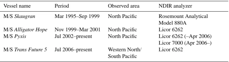
Table 1. Summary of NIES surface ocean CO₂measurements made by four volunteer observing ships in the Pacific Ocean.

Vessel name Period Observed area NDIR analyzer

M/S Skaugran Mar 1995–Sep 1999 North Pacific Rosemount Analytical Model 880A

M/S Alligator Hope Nov 1999–Mar 2001 North Pacific Licor 6262

M/S Pyxis Jul 2002–present North Pacific Licor 6262 (–Apr 2006) Licor 7000 (Apr 2006–) M/S Trans Future 5 Jul 2006–present Western North/

South Pacific

Licor 6262

corresponding SST, MLD, CHL, and SSS values were used. We utilized a subset of the North Pacific dataset collected by the NIES VOS program. ThepCOsea₂ data are available for public use from NIES’s SOOP website: http://soop.jp. Information related to the four VOS lines is summarized in Table 1, and their composite cruise routes are depicted in Fig. 3. The commercial ships collaborating in the NIES VOS program have taken part in trans-Pacific cruises be-tween Japan and North America (10 to 55◦N, 140 to 230◦E) since March 1995 and between Japan and Oceania (45◦S to 35◦N, 140 to 180◦E) since July 2006. The ships sail reg-ularly at intervals of about 5–8 weeks between Japan and North America or Oceania. On the North America route the volunteer ship sailed to the northern part of North America in the early part of the NIES VOS program, but since 2003 the route has occasionally shifted to the southeast to pass through the Panama Canal (Supplement Fig. 1). On the Oceania route the volunteer ship has sailed regularly on a biweekly basis, with the shipping route mostly fixed since July 2006.

Although we reconstructedpCOsea₂ in the North Pacific af-ter 2002, in the analysis we used some in situ data for years 1998–2001 due to the insufficient data coverage especially in the subarctic region for years 2002–2008. The addition of pCOsea₂ data from 1998 to 2001 to the labeling dataset im-proved the coverage of monthly measurements (Supplement, Fig. 2). The improved coverage facilitated reproduction of the rapid drawdown ofpCOsea₂ due to phytoplankton photo-synthesis during the spring bloom in the highly productive western mid–high latitude region.

Murphy et al. (2001b) and Fransson et al. (2006) have both described the technical intricacies of the ocean surface CO2 measurement system used by the NIES VOS program; there-fore we only outline the basics here. The nondispersive in-frared analyzer used for those measurements was changed from a Licor 6262 to a Licor 7000 for the M/S Pyxis cruises in 2006 (Table 1). The CO2standard gases were calibrated by the NIES, and are traceable to the World Meteorologi-cal Organization sMeteorologi-cale. The flow-through tandem equilibrator provides a continuouspCOsea₂ output with high temporal res-olution (Murphy et al., 2001b). ThepCOsea₂ measurements were made every 10 s, and thepCOsea₂ data were 10 min av-erages of those measurements. ThepCOsea₂ data were then

averaged on a daily basis within 0.25◦latitude × 0.25◦ lon-gitude grid boxes. Consequently, the number ofpCOsea₂ data by the NIES VOS program amounted to 317 332, and a total of 73 284pCOsea₂ data were binned as the labeling dataset.

2.4 Other oceanic CO2datasets used for the validation

of estimatedpCOsea₂

To validatepCOsea₂ values reconstructed by the SOM analy-sis, we used the fugacity of oceanic CO2 (fCOsea₂ )dataset from the Surface Ocean CO2 ATlas (SOCAT: http://www. socat.info) version 1.5 database. That dataset has been in the public domain since September 2011, and has been sub-ject to quality control as a part of an international collabo-ration of more than 10 institutes (including NIES) that work on ocean surface CO2 observations (Pfeil et al., 2013). In the North Pacific, the SOCAT database contains thefCOsea₂ values measured mainly by NIES, the Japan Meteorological Agency (JMA), the Japan Agency for Marine-Earth Science and Technology (JAMSTEC), and the United States National Oceanic and Atmospheric Administration (NOAA). For con-sistency with other datasets used in this study we recalculated pCOsea₂ values from the obtainedfCOsea₂ (Pfeil et al., 2013) wherever necessary.

Underway pCOsea₂ data and mooring pCOsea₂ data col-lected by Wong and Johannessen (2010) and Sabine et al. (2010), respectively, were obtained from the Carbon Dioxide Information Analysis Center (CDIAC; http://cdiac. ornl.gov/oceans/). We used those data for the comparisons near ocean station P. In addition, we used pCOsea₂ values calculated from measurements of dissolved inorganic carbon (DIC) and total alkalinity (TA) at two stations: station KNOT (44◦N, 155◦E, Wakita et al., 2010) and station ALOHA (23◦N, 202◦E, Dore et al., 2009).

2.5 Ranges of the training/labeling dataset

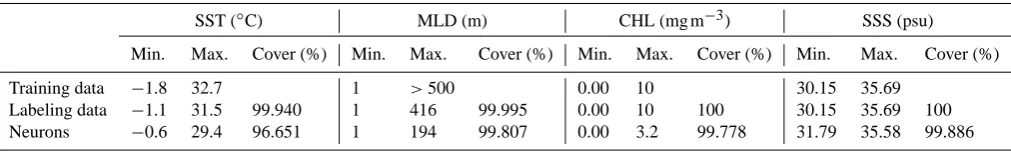
Table 2. Ranges of SST, MLD, CHL, and SSS in the training dataset, the labeling dataset, and the trained neurons. Percentages of the training

data within the range of the labeling dataset and the neurons are given for each parameter.

SST (◦C) MLD (m) CHL (mg m−3) SSS (psu)

Min. Max. Cover (%) Min. Max. Cover (%) Min. Max. Cover (%) Min. Max. Cover (%)

Training data −1.8 32.7 1 >500 0.00 10 30.15 35.69 Labeling data −1.1 31.5 99.940 1 416 99.995 0.00 10 100 30.15 35.69 100 Neurons −0.6 29.4 96.651 1 194 99.807 0.00 3.2 99.778 31.79 35.58 99.886

overlap, determines whether the SOM will be able to re-construct the distribution of the predicted parameter. Ranges of the training/labeling datasets and the trained neurons are summarized in Table 2. The training dataset SSTs varied be-tween−1.8 and 32.7◦C; the MLD ranged from 1 m to more than 500 m; CHL varied from 0 to more than 10 mg m−3; and the range of SSS was 30.15–35.69. The values in the label-ing datasets and neurons covered most of the range of val-ues in the training dataset. However, the maximum MLDs in the labeling dataset (416 m) and in the neurons (194 m) were substantially lower than the maximum MLD in the training dataset (>500 m, Table 2). Our results indicate that the cor-relation betweenpCOsea₂ and MLD was not apparent when the MLD was deeper than 200 m (not shown), a result also reported for the North Atlantic by Telszewski et al. (2009). Therefore the MLD dataset is logarithmically normalized, aligning its weight during training (high weight in low val-ues and low weight in high valval-ues) with its actual influence on the variability inpCOsea₂ . Such normalization means that the MLD change from 10 to 100 m is comparable (in terms of change of weight during training) to that from 100 to 1000 m.

2.6 ReconstructingpCOsea₂ distributions in winter at high latitudes

The three products SST, MLD, and SSS provided full basin-wide coverage from 2002 to 2008. However, the CHL data were affected by the lack of satellite coverage from Novem-ber to January at high latitudes of the North Pacific (north of 45◦N) due to the low angle of the sun during that time and enormous atmospheric correction required to retrieve the sig-nal. To reconstructpCOsea₂ for this area during those months, we assumed thatpCOsea₂ could be adequately characterized by only three parameters: SST, MLD, and SSS. The rationale for this assumption is that biological activity is relatively low during the winter at high latitudes (e.g., Imai et al., 2002). Therefore, we prepared another SOM trained by the three parameters SST, MLD, and SSS. We generated complete pCOsea₂ maps in the study area by combining thepCOsea₂ val-ues obtained with the four-parameter SOM including CHL with the values obtained with the three-parameter SOM ex-cluding CHL in the area north of 45◦N (14 % of the study area) during the period from November to January. We cal-culated the difference between thepCOsea₂ values estimated

with the four-parameter SOM and the three-parameter SOM during the above period in the region between 40 and 45◦N and found it to be−2.0±2.2 µatm. We added this difference to thepCOsea₂ values obtained with the three-parameter SOM in the area north of 45◦N.

2.7 Uncertainty and improvement of thepCOsea₂ estimate

2.7.1 Uncertainty

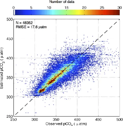
For each in situ pCOsea₂ measurement, the corresponding SOM pCOsea₂ estimate was determined on the basis of the spatial (0.25◦ longitude×0.25◦ latitude grid) and tempo-ral (daily intervals between 1 January 2002 and 31 Decem-ber 2008) coordinates associated with the measurement. We calculated the root-mean-square error (RMSE) between ob-servedpCOsea₂ and estimatedpCOsea₂ values as follows:

RMSE=

s P

pCOsea₂ (estimate)−pCOsea₂ (observed)2

n , (3)

Fig. 4. Scatter plot of estimatedpCOsea₂ with observedpCOsea₂ . Colors indicate the number of data in a 1 µatm×1 µatm bin.

pCOsea₂ in the North Pacific during the spring–summer pe-riod in 1998, and reported that the derivedpCOsea₂ agreed with the shipboardpCOsea₂ observations to within an RMSE of 17–23 µatm.

2.7.2 Changes in the estimate scheme

We have implemented two major improvements over the pre-vious attempt to utilize SOM neural network to compute the pCOsea₂ distribution. In the first one, we followed the suggestion of Telszewski et al. (2009) and Friedrich and Oschlies (2009b) to use the SSS dataset as one of the train-ing datasets to improve pCOsea₂ estimates. The motivation behind using this parameter lies in thepCOsea₂ dependence on (besides other factors) total alkalinity, which for most parts of the global ocean, including the North Pacific, can be accurately approximated from SSS. The SOM technique makes very good use of this relationship, and improvements inpCOsea₂ estimates are seen throughout the basin and are especially apparent in high-gradient regions as described be-low. Moreover, inclusion of SSS in the SOM analysis may fa-cilitate differentiation between temporal and spatial oceanic variability that could not be elucidated with only SST, MLD, and CHL.

To quantify the improvement achieved by using the SSS dataset, we generated another pCOsea₂ map derived with a three-parameter SOM that excluded SSS and compared the result with the four-parameter SOM result. The RMSE be-tween NIES dataset and the three-parameter SOM estimate was 20.0 µatm. Use of SSS in the training dataset therefore

Fig. 5. Comparison of 7 yr averaged monthlypCOsea₂ distributions from 2002 to 2008 in February (upper) and August (bottom). Fig-ures on the left are the pCOsea₂ distributions estimated from the four-parameter SOM including SSS. Figures on the right were esti-mated from the three-parameter SOM without SSS.

reduced the RMSE by 12 %. ThepCOsea₂ distributions were also improved by the use of the SSS data. To visualize the differences, we mapped 7 yr averaged monthlypCOsea₂ distri-butions in February and August derived with and without in-clusion of SSS in the training dataset (Fig. 5). The estimated pCOsea₂ derived from the three-parameter SOM in February is characterized by a smaller longitudinal difference in mid-latitudes than the pCOsea₂ derived from the four-parameter SOM. Furthermore, use of the four-parameter SOM enabled reconstruction of quite highpCOsea₂ values in August in the eastern low/midlatitude region, where the North Pacific Cur-rent flows, whereas use of the three-parameter SOM failed to reproduce this feature. Figure 6 shows the temporal varia-tion ofpCOsea₂ derived with the two SOMs in the North Pa-cific Current region (36 to 38◦N, 138 to 142◦W). It clearly shows that the agreement between observed and estimated pCOsea₂ values was better for the four-parameter SOM than the three-parameter SOM. The RMSE in the region was proved from 15.9 to 10.6 µatm by inclusion of SSS. The im-provement was especially apparent during the summer, when highpCOsea₂ values (about 400 µatm) were observed.

Taking into account the influence of anthropogenic CO2 emissions on the trend ofpCOsea₂ was the second improve-ment introduced in this study. As described above it was done by adding or subtracting 1.76 µatm yr−1 (4.82×10−3µatm day−1_{)to project observedpCO}sea

Fig. 6. ThepCOsea₂ variations in the area (36–38◦N, 138–142◦W) where the North Pacific Current flows, estimated by the four-parameter SOM including SSS (a) and the three-parameter SOM without SSS (b). The blue lines and the shaded areas indicate the mean values of the estimatedpCOsea₂ and the spatial variability (3-σ) calculated in the area, respectively. Blue circles are the in situpCOsea₂ values obtained from the NIES VOS program. ThepCOsea₂ observations in the target areas include several grid points binned by 0.25◦latitude×0.25◦ longitude resolution, and the bar indicates the spatial variability (1-σ).

153 to 157◦_{E) and the Kuroshio Extension (KE) area (34} to 38◦N, 155.5 to 160.5◦E) were unclear (see in Fig. 1). These regions appear to be the same areas where the re-spectivepCOsea₂ trends are not close to that of atmosphere (Takahashi et al., 2006). This suggests that applying a basin-wide correction of 1.76 µatm yr−1(4.82×10−3µatm day−1) might not be the most advantageous, and a nonuniform ap-proach should be employed in the future where subregion-(province) specific correction should be calculated and ap-plied. Overall in this study, inclusion of the secular trend effect slightly, but statistically significantly (p <0.05), re-duced the RMSE for the whole of the North Pacific.

3 Temporal and spatial variation ofpCOsea₂

3.1 Mapping of 7 yr averaged monthlypCOsea₂ distributions

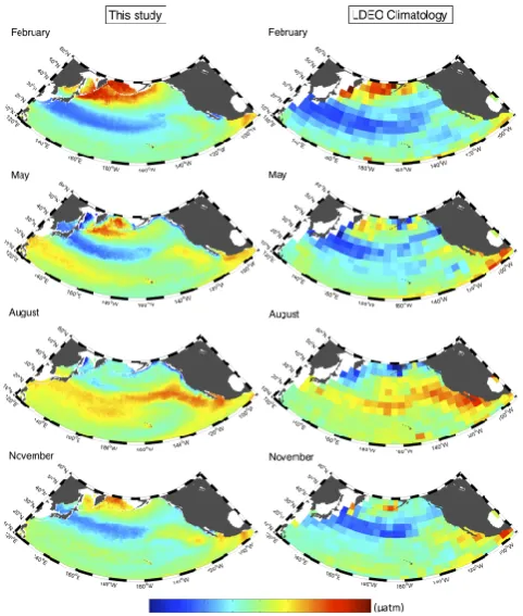
Figure 7 presents a comparison of 7 yr (2002–2008) aver-aged monthlypCOsea₂ distributions derived from SOM re-sults for February, May, August, and November with LDEO pCOsea₂ climatology (Takahashi et al., 2009). The SOM-reconstructedpCOsea₂ distributions in this study clearly show a tongue of very low pCOsea₂ (about 320 µatm) water dis-tributed (except in August) uniformly between the west-ern and central midlatitude regions of the North Pacific (Fig. 7). Such lowpCOsea₂ values are attributed to high rates of photosynthesis (Kameda, 2003) and cooling of the sea-water that occurred mainly in the subtropics. In addition, a band of relatively highpCOsea₂ caused mainly by a sea-sonal rise in temperature was also apparent during the pe-riod from May to September in the western North Pacific between 15 and 30◦N. The temperature rise began in April and amounted to about 2–5◦C. Following the temperature dependence of pCOsea₂ given by Takahashi et al. (1993), δlnpCOsea₂ /δT =0.0423◦C−1, the expectedpCOsea₂ rise due to the temperature effect is about 30–70 µatm. The ob-served increase in expectedpCOsea₂ is only about half of the expected pCOsea₂ rise due to temperature effects. The

in-Fig. 7. Distributions of the 7 yr averaged monthly meanpCOsea₂ in this study (panels on the left) and the LDEO monthlypCOsea₂ climatology (panels on the right, but with 8.8 µatm added to the maps to change the reference year from 2000 to 2005) for February, May, August, and November.

crease may have been attenuated by other factors such as photosynthetic uptake of CO2.

Fig. 8. Difference of thepCOsea₂ between the 7 yr mean pCOsea₂ in this study and the LDEO monthlypCOsea₂ climatology (but with 8.8 µatm added to change the reference year from 2000–2005). Pos-itive values indicate higherpCOsea₂ in this study compared with the LDEO climatology.

values (over 400 µatm) at high latitudes in the North Pa-cific in February; however, the SOM-reconstructedpCOsea₂ distribution shows pCOsea₂ -rich water between the Bering Sea and the coast of northern Japan along the axis of the cold, southward-flowing Eastern Kamchatka Current. As de-scribed in Sect. 2.7.2, high pCOsea₂ values are apparent from June to October in the eastern low/midlatitude region, where the North Pacific Current and the California Cur-rent flow, and the high pCOsea₂ field dominates. With re-spect to the coastal region, low estimates ofpCOsea₂ stretch along the coastline from the Aleutian Islands to the Califor-nia Peninsula from May to October, when the concentration of phytoplankton is high.

The map of differences between SOM results and LDEO climatology for reference year 2005 is shown in Fig. 8. The difference distribution is positive in the western subarctic and the western subtropics and negative in the central-eastern subtropics, the calculated monthly mean difference is close to zero (−0.8 µatm), and its standard deviation is 11.2 µatm.

3.2 Reproducibility of temporalpCOsea₂ variations in each of six regions

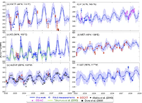
To facilitate a discussion about the temporal variations of pCOsea₂ in the North Pacific, Fig. 9 shows the time series of area-averagedpCOsea₂ estimated in this study for six specific regions of the North Pacific along with observations made during several campaigns at these locations as well as com-puted estimates of Takamura et al. (2010). The grid size of all the averaged areas except in the station KNOT area is set to 4◦_latitude×5◦_{longitude, whereas the station KNOT area} is set to 43.5 to 44.5◦N, 153 to 157◦E to exclude the tran-sition zone between the Kuroshio and the Oyashio. The es-timatedpCOsea₂ values at each location generally agree well with observed values and other estimates, with most of the data lying within the spatial variability (triple the spatial stan-dard deviation: 3-σ) calculated for each area. However dis-agreements greater than 20 µatm between estimatedpCOsea₂

Fig. 9. Interannual variation ofpCOsea₂ (µatm) within time-series station areas and within ocean areas. The blue solid lines and shaded areas show the monthlypCOsea₂ values and the spatial variability (3-σ) calculated in the respective areas. The grid size of all the aver-aged areas except in the station KNOT area is set to 4◦latitude×5◦ longitude, whereas the station KNOT area is set to 43.5–45.5◦N, 153–157◦E. Blue circles and red dots are in situpCOsea₂ values ob-tained from NIES measurements and the SOCAT database, respec-tively. Black dots and crosses on panel (a) and (c) are thepCOsea₂ values calculated from measurements of DIC and TA reported by Wakita et al. (2010) and Dore et al. (2009), respectively. Purple dots on panel (b) are thepCOsea₂ values observed by Wong and Johan-nessen (2010) and Sabine et al. (2010). In panel (c), the solid green line denotes thepCOsea₂ values during the 2002–2006 period esti-mated by Takamura et al. (2010). Note that the range of the ordinate in the station KNOT area is larger than those of other station areas.

Fig. 10. Anomalies from the monthly climatology for the period

box 2002–2008 for detrendingpCOsea₂ (upper), SST (middle), and MLD (bottom) distributions during the winter of 2003 (panels on the left) and 2008 (panels on the right).

pCOsea₂ values in the eastern subtropics (EST) area (14 to 18◦N, 115.5 to 119.5◦W) also agree well with the data from the NIES VOS program (Fig. 9f). As shown in Fig. 9d–f, the patterns of variation were similar in the WST, station ALOHA, and EST areas. Keeping in mind that only data ob-tained by the NIES VOS program were used in the SOM la-beling process, these results suggest that the lala-beling process allows for labeled SOM neurons to effectively learnpCOsea₂ variations from pCOsea₂ values observed in other subtropi-cal areas. This confirms the earlier suggestions that the SOM technique, to a larger extent than more traditional mapping techniques, overcomes problems associated with temporal and spatial scarcity of the labeling data (in situ) by putting significant weight on the availability and quality of the train-ing data (satellite and assimilation).

Finally, as an additional independent validation exercise, we calculated the RMSE between all the independent data visualized in Fig. 9 and equivalent SOM estimates. Such a calculated uncertainty estimate turns out to be 20.1 µatm, al-most identical to that obtained for SOCAT dataset, giving more confidence in our error estimate.

3.3 Difference ofpCOsea₂ distributions during ENSO events

The ENSO has a large influence on the climate of the North Pacific (IPCC, 2007), and large fluctuations ofpCOsea₂ co-incided with the ENSO cycle have also been observed in the

equatorial Pacific (Feely et al., 2006; Ishii et al., 2009). Based on their measurements from 1983 to 2003, Midorikawa et al. (2006) have suggested that the interannual variation of pCOsea₂ in the western subtropical North Pacific is also re-lated to the ENSO. Although the extent of the ENSO influ-ence on oceanic and atmospheric variables is known to be global (Trenberth and Caron, 2000), the impact of the ENSO on the distribution of pCOsea₂ over the entire area of the North Pacific is not well understood. Figure 10 depicts the estimated distributions of the detrendedpCOsea₂ , SST, and MLD anomalies during the winters of 2003 (i.e., El Niño) and 2008 (i.e., La Niña). Anomalies in Fig. 10 are deviations from the monthly climatology for the period of 2002–2008. El Niño/La Niña periods were chosen in accordance with JMA’s definition based on the 5-month running mean SST deviation for the NINO.3 region (5◦_{S to 5}◦_{N, 90 to 150}◦_W). The patterns of SST anomalies in Fig. 10 are typical of El Niño and La Niña winters (Trenberth and Caron, 2000; Alexander et al., 2002). The pCOsea₂ anomaly related to ENSO events is easily discernible in the western-central sub-tropical region, in the eastern subarctic region, and in the eastern midlatitude region south of 30◦N. For example, a negativepCOsea₂ anomaly is apparent in the western-central subtropical region in 2003 (El Niño), when the SST anomaly was negative, whereas a positivepCOsea₂ anomaly is appar-ent in 2008 (La Niña), when the SST anomaly is positive. The opposite pattern is observed for the eastern midlati-tude region south of 30◦N. The amplitudes of the associated pCOsea₂ anomalies are about 15 µatm, and their SST ampli-tudes are 1◦C. ThepCOsea₂ change closely tracked the SST change in accordance with the iso-chemical temperature de-pendency of Takahashi et al. (1993).

4 Summary

In this study we used the SOM technique of Telszewski et al. (2009) to examine the temporal and spatial variations of pCOsea₂ in the North Pacific during the period 2002–2008. To improve thepCOsea₂ estimates, we used SSS as an addi-tional training parameter and assumed a trend of increasing pCOsea₂ to take into account the effect of anthropogenic CO2 emissions onpCOsea₂ . The estimated results revealed that the SOM technique could satisfactorily reconstruct variations of pCOsea₂ associated with bio-geophysical processes expressed by the variability in four proxy parameters: SST, MLD, CHL, and SSS. We calculated the uncertainty of thepCOsea₂ esti-mation to be from 17.8 µatm for the NIES labeling dataset to 20.2 µatm for the SOCAT dataset. The fact that the un-certainty was reduced by about 12 % by inclusion of SSS in the training dataset suggests that SSS can be a useful pa-rameter for the estimation of temporal and spatial variation ofpCOsea₂ . We also found thatpCOsea₂ estimates were im-proved by taking account of the temporal trend associated with anthropogenic CO2emissions.

The calculatedpCOsea₂ variations in six ocean areas gen-erally agreed well not only with the NIES VOS program pCOsea₂ data used for the labeling process but also with other in situpCOsea₂ datasets. Seven-year (2002–2008) averaged monthlypCOsea₂ distributions were similar to 35 yr climatol-ogypCOsea₂ distributions (Takahashi et al., 2009). However, the SOM-basedpCOsea₂ mapping, with its high spatial reso-lution, reflected oceanic conditions with more detail. The es-timated interannualpCOsea₂ variability revealed a difference in the spatial pattern ofpCOsea₂ during the winter of the El Niño period in 2003 and the La Niña period in 2008. A neg-ativepCOsea₂ anomaly was apparent in 2003 in the western subtropical North Pacific and in the eastern subarctic North Pacific off the coast of Alaska, whereas a positive anomaly was apparent in 2008 in the same regions. In the western subtropical and eastern midlatitude regions, the correlation of the pCOsea₂ variability with ENSO events seemed to be related mainly to changes in the thermodynamic properties of seawater. In contrast, similar correlation in the subarc-tic North Pacific seemed to be related to changes in versubarc-tical transport of CO2-rich subsurface waters.

Further improvement ofpCOsea₂ estimates will most cer-tainly require an increase in the number of data points used for labeling. With new datasets becoming available (SOCAT version 2 and LDEO V2012) and offering relatively dense annual data coverage in several oceans regions, we are now in a position to commence a sensitivity study allowing for a meaningful quantitative assessment to be made of the uncer-tainty related to the amount of labeling data utilized during the mapping process. In this study, 7 % of the neurons were not labeled, suggesting that in situ measurements covering a wider range of environmental conditions (as approximated by SST, MLD, CHL, and SSS) are needed to enable the full mapping potential of the method. We plan to undertake a

longer-term study covering global ocean using the commu-nity quality-controlled (Pfeil et al., 2013) SOCAT collection as the labeling dataset. This work will include a sensitivity study hopefully allowing for quantification of the relation-ship between the amount of the in situ data and the method’s uncertainty estimate.

The number of neurons is also crucial for accuratepCOsea₂ estimation. In this study we used three times as many neurons as Telszewski et al. (2009) to achieve adequate reproducibil-ity of thepCOsea₂ estimates. However, the number of neu-rons used in this study was based on the available comput-ing power rather then determined by scientific need. It might also be possible to improve thepCOsea₂ estimate by inclusion of more ocean parameters. Sea surface height is a potential training parameter with basin-wide coverage.

In addition to estimates in the North Pacific, long-term global pCOsea₂ mapping based on such measurements is also important for understanding interannual variations of air–sea CO2exchanges. AlthoughpCOsea₂ variations related to climate changes such as the PDO have been reported (Valsala et al., 2012), the overall impact of such changes on globalpCOsea₂ variations is not well understood. In the present study, the study area was confined to the North Pa-cific. However, the SOM technique used in the present study has the potential to estimatepCOsea₂ in regions where there are insufficient numbers of observations, and such regions will be our next target. It is axiomatic to say that further pCOsea₂ measurements are critical, especially in the South Pacific, where fewpCOsea₂ measurements have been made (Sabine et al., 2013).

Supplementary material related to this article is available online at http://www.biogeosciences.net/10/ 6093/2013/bg-10-6093-2013-supplement.pdf.

Acknowledgements. We deeply appreciate the generous

coop-eration of Seaboard International Shipping Co., Mitsui O. S. K. Lines Co., Toyofuji Shipping Co., and Kagoshima Senpaku Co. with the NIES VOS program. We would like to thank the crew of the M/S Skaugran, M/S Alligator Hope, M/S Pyxis, and M/S

Trans Future 5. We also thank S. Kariya and T. Yamada of the

Global Environmental Forum for their constant assistance with the observations, and appreciate the work of K. Katsumata for calibrating the CO₂standard gases. We are thankful to contributors of the SOCAT database and the CDIAC database for providing oceanic CO₂data. We gratefully acknowledge Mercator Ocean for providing the GLORYS model output. The research was financially supported by the Global Environment Research Account for National Institutes by the Ministry of Environment, Japan. Finally, we also express our deep thanks to R. Wannikhof, A. Lenton, and two anonymous reviewers, who provided us with many useful comments.

References

Alexander, M. A., Blade, I., Newman, M., Lanzante, J. R., Lau, N.-C., and Scott, J. D.: The atmospheric bridge: The influence of ENSO teleconnections on air-sea interaction over the global oceans, J. Climate, 15, 2205–2231, 2002.

Bates, N. R.: Interannual variability of the oceanic CO2 sink in the subtropical gyre of the North Atlantic Ocean over the last 2 decades, J. Geophys. Res., 112, C09013, doi:10.1029/2006JC003759, 2007.

Bates, N. R., Best, M. H. P., Neely, K., Garley, R., Dickson, A. G., and Johnson, R. J.: Detecting anthropogenic carbon dioxide uptake and ocean acidification in the North Atlantic Ocean, Bio-geosciences, 9, 2509–2522, doi:10.5194/bg-9-2509-2012, 2012. Bernard, B., Madec, G., Penduff, T., Molines, J.-M., Treguier, A.-M., Sommer, J. L., Beckmann, A., Biastoch, A., Böning, C., Dengg, J., Derval, C., Durand, E., Gulev, S., Remy, E., Talandier, C., Theetten, S., Maltrud, M., McClean, J., and Cuevas, B. D.: Impact of partial steps and momentum advection schemes in a global ocean circulation model at eddy-permitting resolution, Ocean Dynam., 56, 543–567, doi:10.1007/s10236-006-0082-1, 2006.

Cooper, D. J., Watson, A. J., and Ling, R. D.: Variation ofpCO2 along a North Atlantic shipping route (UK to the Caribbean): a year of automated observations., Mar. Chem., 72, 151–169, 1998.

Chierici, M., Fransson, A., and Nojiri, Y.: Biogeochemical pro-cesses as drivers of surface fCO2 in contrasting provinces in the subarctic North Pacific Ocean, Global Biogeochem. Cy., 20, GB1009, doi:10.1029/2004GB002356, 2006.

Dore, J. E., Lukas, R., Sadler, D. W., Church, M. J., and Karl, D. M.: Physical and Biogeochemical Modulation of Ocean Acidi-fication in the Central North Pacific, PNAS, 106, 12235–12240, doi:10.1073/pnas.0906044106, 2009.

Dugdale, R. C. and Wilkerson, F. P.: Low specific nitrate uptake rate: A common feature of high-nutrient, low-chlorophyll marine ecosystems, Limnol. Oceanogr., 36, 1678–1688, 1991.

Feely, R. A., Gammon, R. H., Taft, B. A., Pullen, P. E., Waterman, L. S., Conway, T. J., Gendron, J. F., and Wisegarver, D. P.: Distri-bution of chemical tracers in the eastern Equatorial Pacific dur-ing and After the 1982–83 El Nino/Southern Oscillation Event, J. Geophys. Res., 92, 6545–6558, 1987.

Feely, R. A., Takahashi, T., Wanninkhof, R., McPhaden, M. J., Cosca, C. E., Sutherland, S. C., and Carr, M.-E.: Decadal vari-ability of the air-sea CO2fluxes in the equatorial Pacific Ocean, J. Geophys. Res., 111, C08S90, doi:10.1029/2005JC003129, 2006. Ferry, N., Parent, L., Garric, G., Barnier, B., Jourdain, N. C., and the Mercator Ocean team: Mercator Global Eddy Permitting Ocean Reanalysis GLORYS1V1: Description and Results, Mer-cator Ocean Quarterly Newsletter, 36, 15–27, 2010.

Fransson, A., Chierici, M., and Nojiri, Y.: Increased net CO2 out-gassing in the upwelling region of the southern Bering Sea in a period of variable marine climate between 1995 and 2001, J. Geophys. Res., 111, C08008, doi:10.1029/2004JC002759, 2006. Friedrich, T. and Oschlies, A.: Neural network-based esti-mates of North Atlantic surface pCO2 from satellite data: A methodological study, J. Geophys. Res., 114, C03020, doi:10.1029/2007JC004646, 2009a;

Friedrich, T. and Oschlies, A.: Basin-scalepCO₂maps estimated from ARGO float data: A model study, J. Geophys. Res., 114, C10012, doi:10.1029/2009JC005322, 2009b.

GLOBALVIEW-CO2: Cooperative Atmospheric Data Integration Project – Carbon Dioxide, CD-ROM, NOAA ESRL, Boulder, Colorado [Also available on Internet via anonymous FTP to ftp.cmdl.noaa.gov, Path: ccg/co2/GLOBALVIEW], 2011. González-Dávila, M., Santana-Casiano, J. M., Rueda, M. J., and

Llinás, O.: The water column distribution of carbonate system variables at the ESTOC site from 1995 to 2004, Biogeosciences, 7, 3067–3081, doi:10.5194/bg-7-3067-2010, 2010.

Imai, K., Nojiri, Y., Tsurushima, N., and Saino, T.: Time series of seasonal variation of primary productivity at station KNOT (44◦N, 155◦E) in the sub-arctic western North Pacific, Deep-Sea Res. II, 49, 5395–5408, 2002.

Inoue, H. Y., Matsueda, H., Ishii, M., Fushimi, K., Hirota M., Asanuma, I., and Takasugi, Y.: Long-term trend of the partial pressure of carbon dioxide (pCO2)in surface waters of the west-ern North Pacific 1984-1993, Tellus B, 47, 391–413, 1995. IPCC: Climate Change 2007: The Physical Science Basis.

Con-tribution of Working Group I to the Fourth Assessment Report of the Intergovernmental Panel on Climate Change, edited by: Solomon, S., Qin, D., Manning, M., Chen, Z., Marquis, M., Av-eryt, K. B., Tignor, M., and Miller, H. L., Cambridge University Press, Cambridge, United Kingdom and New York, NY, USA, 2007.

Ishii, M., Inoue, H. Y., Midorikawa, T., Saito, S., Tokieda, T., Sasano, D., Nakadate, A., Nemoto, K., Metzl, N., Wong, C. S., and Feely, R. A.: Spatial variability and decadal trend of the oceanic CO2in the western equatorial Pacific warm/fresh water, Deep-Sea Res. II, 56, 591–606, doi:10.1016/j.dsr2.2009.01.002, 2009.

Jamet, C., Moulin, C., and Lefèvre, N.: Estimation of the oceanic pCO2 in the North Atlantic from VOS lines in-situ measure-ments: parameters needed to generate seasonally mean maps, Ann. Geophys., 25, 2247–2257, 2007,

http://www.ann-geophys.net/25/2247/2007/.

Kameda, T.: Studies on oceanic primary production using ocean color remote sensing data, Bull. Fish. Res. Agen., 9, 118–148, 2003.

Karl, D. M. and Letelier, R. M.: Nitrogen fixation-enhanced car-bon sequestration in low nitrate, low chlorophyll seascapes, Mar. Ecol. Prog. Ser., 354, 257–268, doi:10.3354/meps07547, 2008. Kohonen, T.: Self-Organizing Maps. Third, extended edition,

Springer-Verlag, Berlin, Heidelberg, New York, 501 pp., 2001. Kurihara, Y., Sakurai, T., and Kuragano, T.: Global daily sea

sur-face temperature analysis using data from satellite microwave radiometer, satellite infrared radiometer and in-situ observations, Sokko-jiho, 73, S1–S18, 2006.

Lefèvre, N., Watson, A. J., and Watson, A. R.: A comparison of multiple regression and neural network techniques for mapping in situpCO2 data, Tellus, 57B, 375-384, doi:10.1111/j.1600-0889.2005.00164.x, 2005.

Lewis, E. and Wallace, D. W. R.: Program Developed for CO2 System Calculations. ORNL/CDIAC-105. Carbon Diox-ide Information Analysis Center, Oak Ridge National Lab-oratory, U.S. Department of Energy, Oak Ridge, Tennessee, doi:10.3334/CDIAC/otg.CO2SYS_DOS_CDIAC105, 1998. Midorikawa, T., Ishii, M., Nemoto, K., Kamiya, H., Nakadate, A.,

Masuda, S., Matsueda, H., Nakano, T., and Inoue, H. Y.: Inter-annual variability of winter oceanic CO2and air-sea CO2flux in the western North Pacific for 2 decades, J. Geophys. Res., 111, C07S02, doi:10.1029/2005JC003095, 2006.

Miller, L. A., Christian, J., Davelaar, M., Johnson, W. K., and Linguanti, J.: Carbon Dioxide, Hydrographic and Chem-ical Data Obtained During the Time Series Line P Cruises in the North-East Pacific Ocean from 1985–2010, http:// cdiac.ornl.gov/ftp/oceans/CLIVAR/Line_P.data/, Carbon Diox-ide Information Analysis Center, Oak Ridge National Lab-oratory, US Department of Energy, Oak Ridge, Tennessee, doi:10.3334/CDIAC/otg.CLIVAR_Line_2009, 2010.

Murphy, P. P., Nojiri, Y., Fujinuma, Y., Wong, C. S., Zeng, J., Ki-moto, T., and KiKi-moto, H.: Measurements of Surface Seawater fCO2from Volunteer Commercial Ships: Techniques and Expe-riences from Skaugran, J. Atmos. Ocn. Tech., 18, 1719–1734, 2001a.

Murphy, P. P., Nojiri, Y., Harrison, D. E., and Larkin, N. K.: Scales of spatial variability for surface ocean pCO2 in the Gulf of Alaska and Bering Sea: toward a sampling strategy, Geophys. Res. Lett., 28, 1047–1050, 2001b.

Olsen, A., Bellerby, R. G. J., Johannessen, T., Omar, A., and Skjel-van, I.: Interannual variability in the wintertime air-sea flux of carbon dioxide in the northern North Atlantic, 1981–2001, Deep-Sea Res. I, 50, 1323–1338, 2003.

O’Reilly, J. E., Maritorena, S., Siegel, D., O’Brien, M. C., Toole, D., Mitchell, B. G., Kahru, M., Chavez, F. P., Strutton, P., Cota, G., Hooker, S. B., McClain, C. R., Carder, K.L., Muller-Karger, F., Harding, L., Magnuson, A., Phinney, D., Moore, G. F., Aiken, J., Arrigo, K. R., Letelier, R., and Culver, M.: Ocean color chloro-phyll a algorithms for SeaWiFS, OC2, and OC4: Version 4, in: SeaWiFS Postlaunch Technical Report Series, edited by: Hooker, S. B and Firestone, E. R., Vol. 11, SeaWiFS Postlaunch Cali-bration and Validation Analyses, Part 3. NASA, Goddard Space Flight Center, Greenbelt, Maryland, 9–23, 2000.

Patra, P. K., Maksyutov, S., Ishizawa, M., Nakazawa, T., Takahashi, T. and Ukita, J.: Interannual and decadal changes in the sea-air CO₂flux from atmospheric CO₂inverse modeling, Global Bio-geochem. Cy., 19, GB4013, doi:10.1029/2004GB002257, 2005. Pfeil, B., Olsen, A., Bakker, D. C. E., Hankin, S., Koyuk, H., Kozyr, A., Malczyk, J., Manke, A., Metzl, N., Sabine, C. L., Akl, J., Alin, S. R., Bellerby, R. G. J., Borges, A., Boutin, J., Brown, P. J., Cai, W.-J., Chavez, F. P., Chen, A., Cosca, C., Fassbender, A. J., Feely, R. A., González-Dávila, M., Goyet, C., Hardman-Mountford, N., Heinze, C., Hood, M., Hoppema, M., Hunt, C. W., Hydes, D., Ishii, M., Johannessen, T., Jones, S. D., Key, R. M., Körtzinger, A., Landschützer, P., Lauvset, S. K., Lefèvre, N., Lenton, A., Lourantou, A., Merlivat, L., Midorikawa, T., Mintrop, L., Miyazaki, C., Murata ,A., Nakadate, A., Nakano, Y., Nakaoka, Y. Nojiri, A. M. Omar, X. A. Padin, G.-H. Park, K. Paterson, F. F. Perez, S., Pierrot, D., Poisson, A., Ríos, A. F., Salisbury, J., Santana-Casiano, J. M., Sarma, V. V. S. S., Schlitzer, R., Schneider, B., Schuster, U., Sieger, R., Skjelvan, I.,

Steinhoff, T., Suzuki, T., Takahashi, T., Tedesco, K., Telszewski, M., Thomas, H., Tilbrook, B., Tjiputra, J., Vandemark, D., Ve-ness, T., Wanninkhof, R., Watson, A. J., Weiss, R., Wong, C. S., and Yoshikawa-Inoue, H.: A uniform, quality controlled Surface Ocean CO2Atlas (SOCAT), Earth Syst. Sci. Data, 5, 125–143, doi:10.5194/essd-5-125-2013, 2013.

Robbins, L. L., Hansen, M. E., Kleypas, J. A., and Meylan, S. C.: CO2calc – A user-friendly seawater carbon calculator for Win-dows, Max OS X, and iOS (iPhone): U.S. Geological Survey Open-File Report 2010–1280, p. 17, 2010.

Sabine, C. L., Feely, R. A., Gruber, N., Key, R. M., Lee, K., Bullis-ter, J. L., Wanninkhof, R., Wong, C. S., Wallace, D. W. R., Tilbrook, B., Millero, F. J., Peng, T.-H., Kozyr, A., Ono, T., and Rios, A. F.: The Oceanic Sink for Anthropogenic CO2, Science, 305, 367–371, doi:10.1126/science.1097403, 2004.

Sabine, C. L., Maenner, S., and Sutton, A.: High-resolution ocean and atmosphere pCO2 time-series measurements from mooring Papa_145W_50N, Carbon Dioxide Infor-mation Analysis Center, Oak Ridge National Labora-tory, US Department of Energy, Oak Ridge, Tennessee, doi:10.3334/CDIAC/otg.TSM_Papa_145W_50N, 2010. Sabine, C. L., Hankin, S., Koyuk, H., Bakker, D. C. E., Pfeil, B.,

Olsen, A., Metzl, N., Kozyr, A., Fassbender, A., Manke, A., Malczyk, J., Akl, J., Alin, S. R., Bellerby, R. G. J., Borges, A., Boutin, J., Brown, P. J., Cai, W.-J., Chavez, F. P., Chen, A., Cosca, C., Feely, R. A., González-Dávila, M., Goyet, C., Hardman-Mountford, N., Heinze, C., Hoppema, M., Hunt, C. W., Hydes, D., Ishii, M., Johannessen, T., Key, R. M., Körtzinger, A., Landschützer, P., Lauvset, S. K., Lefèvre, N., Lenton, A., Lourantou, A., Merlivat, L., Midorikawa, T., Mintrop, L., Miyazaki, C., Murata, A., Nakadate, A., Nakano, Y., Nakaoka, S., Nojiri, Y., Omar, A. M., Padin, X. A., Park, G.-H., Pater-son, K., Perez, F. F., Pierrot, D., PoisPater-son, A., Ríos, A. F., Sal-isbury, J., Santana-Casiano, J. M., Sarma, V. V. S. S., Schlitzer, R., Schneider, B., Schuster, U., Sieger, R., Skjelvan, I., Stein-hoff, T., Suzuki, T., Takahashi, T., Tedesco, K., Telszewski, M., Thomas, H., Tilbrook, B., Vandemark, D., Veness, T., Watson, A. J., Weiss, R., Wong, C. S., and Yoshikawa-Inoue, H.: Surface Ocean CO2Atlas (SOCAT) gridded data products, Earth Syst. Sci. Data, 5, 145–153, doi:10.5194/essd-5-145-2013, 2013. Sarma, V. V. S. S., Saino, T., Sasaoka, K., Nojiri, Y., Ono, T., Ishii,

M., Inoue, H. Y., and Matsumoto, K.: Basin-scalepCO₂ distribu-tion using satellite sea surface temperature, Chl-a, and climato-logical salinity in the North Pacific in spring and summer, Global Biogeochem. Cy., 20, GB3005, doi:10.1029/2005GB002594, 2006.

Schmitz, W. J. Jr.: On the World Ocean Circulation: Volume I; Some Global Features/North Atlantic Circulation, edited by: Rept., Tech., Woods Hole Oceanogr. Inst., Woods Hole, Massachusetts 02543, 1996.

Schuster, U., Watson, A. J., Bates, N. R., Corbiére, A., González-Dávila, M., Metzl, N., Pierrot, D., and Santana-Casiano, M.: Trends in North Atlantic sea-surfacefCO2from 1990 to 2006, Deep-Sea Res. II, 56, 620–629, 2009.

Stephens, M. P., Samuels, G., Olson, D. B., Fine, R. A., and Taka-hashi, T.: Sea-air flux of CO2in the North Pacific using shipboard and satellite data, J. Geophys. Res., 100, 13571–13583, 1995. Takahashi, T., Olafsson, J., Godard, J. G., Chipman, D. W., and

high-latitude surface oceans: A comparative study, Global Bio-geochem. Cy., 7, 843–878, 1993.

Takahashi, T., Sutherland, S. C., Feely, R. A., and Wanninkhof, R.: Decadal change of the surface waterpCO2in the North Pacific: A synthesis of 35 years of observations, J. Geophys. Res., 111, C07S05, doi:10.1029/2005JC003074, 2006.

Takahashi, T., Sutherland, S. C., Wanninkhof, R., Sweeney, C., Feely, R. A., Chipman, D. W., Hales, B., Friederich, G., Chavez, F., Watson, A., Bakker, D. C. E., Schuster, U., Metzl, N., Inoue, H. Y., Ishii, M., Midorikawa, T., Sabine, C. L., Hopemma, M., Olafsson, J., Arnarson, T. S., Tilbrook, B., Jo-hannessen, T., Olsen, A., Bellerby, R., de Baar, H. J. W., No-jiri, Y., Wong, C. S., and Delille, B.: Climatological mean and decadal change in surface ocean pCO2, and net sea-air CO2 flux over the global oceans, Deep-Sea Res. II, 56, 554–577, doi:10.1016/j.dsr2.2008.12.009, 2009.

Takamura, T. R., Inoue ,H. Y., Midorikawa, T., Ishii, M., and No-jiri, Y.: Seasonal and inter-annual variations inpCO2sea and air-sea CO₂fluxes in mid-latitudes of the western and eastern North Pacific during 1999-2006: Recent results utilizing volun-tary observation ships, J. Meteorol. Soc. Japan, 88, 883–898, doi:10.2151/jmsj.2010-602, 2010.

Telszewski, M., Chazottes, A., Schuster, U., Watson, A. J., Moulin, C., Bakker, D. C. E., González-Dávila, M., Johannessen, T., Körtzinger, A., Lüger, H., Olsen, A., Omar, A., Padin, X. A., Ríos, A. F., Steinhoff, T., Santana-Casiano, M., Wallace, D. W. R., and Wanninkhof, R.: Estimating the monthlypCO2 distri-bution in the North Atlantic using a self-organizing neural net-work, Biogeosciences, 6, 1405–1421, doi:10.5194/bg-6-1405-2009, 2009.

Trenberth, K. E. and Caron, J. M.: The Southern Oscillation revis-ited: Sea level pressures, surface temperatures and precipitation, J. Climate, 13, 4358–4365, 2000.

Usui, N., Ishizaki, S., Fujii, Y., Tsujino, H., Yasuda, T., and Ka-machi, M.: Meteorological Research Institute multivariate ocean variational estimation (MOVE) system: Some early results, Adv. Space Res., 37, 806–822, doi:10.1016/j.asr.2005.09.022, 2006. Valsala, V., Maksyutov, S., Telszewski, M., Nakaoka, S., Nojiri, Y.,

Ikeda, M., and Murtugudde, R.: Climate impacts on the struc-tures of the North Pacific air-sea CO₂flux variability, Biogeo-sciences, 9, 477–492, doi:10.5194/bg-9-477-2012, 2012. Wakita, M., Watanabe, S., Murata, A., Tsurushima, N., and Honda,

M.: Decadal change of dissolved inorganic carbon in the sub-arctic western North Pacific Ocean, Tellus B, 62, 608–620, doi:10.1111/j.1600-0889.2010.00476.x, 2010.

Wong, C. S. and Johannessen, S.: Sea surface and atmospheric pCO2 data in the Pacific Ocean during the station P cruises from 1973–2003., Carbon Dioxide Information Analysis Center, Oak Ridge National Laboratory, US Department of Energy, Oak Ridge, Tennessee, doi:10.3334/CDIAC/otg.VOS_station_p_ca, 2010.

Wong, C. S., Christian, J. R., Emmy Wong, S.-K., Page, J., Xie, L.,and Johannessen, S.: Carbon dioxide in surface seawater of the eastern North Pacific Ocean (Line P), 1973-2005, Deep-Sea Res. I, 57, 687–695, doi:10.1016/j.dsr.2010.02.003, 2010. Zeng, J., Nojiri, Y., Murphy, P. P., Wong, C. S., and Fujinuma, Y.: A