A basic general model of vector-borne diseases

(1)

https://doi.org/10.28919/cmbn/3485 ISSN: 2052-2541

A BASIC GENERAL MODEL OF VECTOR-BORNE DISEASES

S. Y. TCHOUMI1,∗, J. C. KAMGANG2, D. TIEUDJO2, G. SALLET3,

1_{Department of Mathematics and Computer Sciences, Faculty of Sciences, University of Ngaoundere, P. O. Box}

454, NGaoundere, Cameroon

2_{Department of Mathematics and Computer Sciences, ENSAI – University of NGaoundere, P. O. Box 455}

NGaoundere, Cameroon

3_{INRIA-Lorraine and Laboratoire de Mathmatiques et Applications de Metz UMR CNRS 7122, University of}

Metz, 57045 Metz Cedex 01, France

Communicated by S. Shen

Copyright c2018 Tchoumi, Kamgang, Tieudjo and Sallet. This is an open access article distributed under the Creative Commons Attribution License, which permits unrestricted use, distribution, and reproduction in any medium, provided the original work is properly cited.

Abstract.We propose a model that can translate the dynamics of vector-borne diseases, for this model we compute the basic reproduction number and show that ifR0<ζ<1 the DFE is globally asymptotically stable. ForR0>1

we prove the existence of a unique endemic equilibrium and ifR0≤1 the system can have one or two endemic

equilibrium, we also show the existence of a backward bifurcation. By numerical simulations we illustrate with

data on malaria all the results including existence, stability and bifurcation.

Keywords: epidemiological model; sensitivity analysis; basic reproduction number; global asymptotic stability; bifurcation; simulation.

2010 AMS Subject Classification:92B05.

∗_{Corresponding author}

E-mail address: sytchoumi83@gmail.com

Received August 26, 2017

(2)

1. Introduction

The vector-borne diseases are responsible for more than 17% of infectious diseases, and

causes over one million deaths each year [18]. Mathematical models help to better understand

and propose solutions to reduce the negative impact of these disease in society, and several

studies have already been made on diseases such as malaria, leishmaniasis, trypanosomiasis

just to name a few (see [15, 6, 19, 16, 1, 2, 10, 11]). We realise that the behavior of these

diseases can be modeled by a generic model. Thus in this first work, we propose a model of one

population that can translate the dynamics of several vector-borne diseases.

We take a different approach in modeling vectors, drawing on the work Ngwa, Ngonghala

[8, 4, 5] which integrates the three phases of the gonotrophic cycle. We assume as in [13] that

rest and laying occur in the same place ie we have a questing phase and another phase resting.

In addition to the consideration of the gonotriphic cycle, we integrate the management of the

sporogonic cycle, that is to say that we consider the fact that after the first meal infecting the

vector can transmit the disease only after a certain number of meals (This number depends on

the species). In the population of host we introduce the two parametersu,v∈ {0,1} opposite to [12] where u,v∈]0,1[ thereby controlling the presence or absence of the compartments E of exposed and Rof immune. This allows us to place ourselves in one ofSIS, SIRS, SEISor

SEIRSdynamics, we study the existence and stability of equilibrium and the bifurcation.

2. Model description and mathematical specification

In our model, we consider two populations, namely a population of host which may be

hu-mans or animals and a vector population that can be specified according to the disease that one

wishes to model.

2.1. Host population structure and dynamics

The host population is subdivided in four compartments: susceptible, infected, infectious

(3)

the dynamics in the host population. Thus according to the values ofuand vwe can have the

dynamicsSIS,SIRS,SEISorSEIRS.

FIGURE 1. Dynamics in the host population

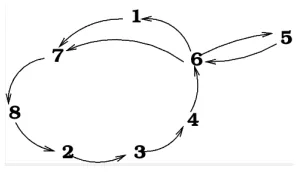
2.2. Mosquito population structure and dynamics

In the vector population we adopt the questing-resting as described in [13], but to simplify

the calculations we consider the questing-resting phase number equal to 1. The figure below

illustrates the dynamics in Population of vectors.

FIGURE 2. Mosquito population dynamics

(4)

TABLE1. Variable of model

Variable Description

humans

Sh Number of susceptible humans in the population Eh Number of infected humans in the population I_h Number of infectious humans in the population

Rh Number of immune humans in the population

mosquitoes

Sq Number of questing susceptible mosquitoes E_qi Number of questing infected mosquitoes in stepi E_ri Number of resting infected mosquitoes in stepi Iq Number of questing infectious mosquitoes Ir Number of resting infectious mosquitoes

TABLE 2. fundamental model parameter

Parameter Description Unity

human

Λh immigration in the host population h×j−1

γ rate of lost of immunity in the host population j−1

λ rate of transition for infected to infectious in the host population j−1

ξ rate of recovery in the host population j−1

µ death rate in the host population j−1

d disease-induced death rate in the host population j−1 a number of bites on humans by a single female mosquito per unit time

m Infectivity coefficient of hosts due to bite of infectious vector variable Mosquitoes

Λv imigration of vectors m×j−1

χ Rate at which resting vectors move to the questing state j−1 β Rate at which quessting vectors move to the resting state j−1

κ death rate of resting vectors j−1

κ 0

death rate of questing vectors j−1

c Infectivity coefficient of vector due to bite of infectious host . variable ˜

(5)

TABLE 3. Derived model parameters

Param. Formula Description

α amIQ

Nh

incidence rate of susceptible human

ϕ acIh

Nh

+avcR˜ h Nh

incidence rate of susceptible mosquitoes

2.3. Model equation

The diagrams (1) and (2) allow us to have the following system of equations:

(1)                                                                                                              ˙

S_h = Λh+vγRh+v˜ξIh−(µ+α)Sh v˜=1−v

˙

E_h = u[αSh−(µ+λ)Eh]

˙

I_h = uλEh+u˜αSh−[µˆ +ξ]Ih µˆ =µ+d; u˜=1−u

˙

R_h = v[ξIh−(µ+γ)Rh]

˙

S_q = Λv−(κ

0

+ϕ)Sq

˙

E_r0 = ϕSq−(κ+χ)Er0

˙

E_q1 = χE_r0−(κ0+β)E_q1

˙

E_r1 = βE_q1−(κ+χ)E_r1

˙

I_q = χE_r1−(κ0+β)Iq+χIr

˙

(6)

3. Well-posedness, dissipativity

In this section we demonstrate well-posedness of the model by demonstrating invariance

of the set of non-negative states, as well as boundedness properties of the solution. We also

calculate the equilibria of the system.

3.1. Positive invariance of the non-negative cone in state space

The system (1) can be rewritten in the matrix form as

(2) x˙ =A(x)x+b(x)⇐⇒  

 ˙

x_S = A_S(x).x_S+A_SI(x)xI+bS ˙

xI = AI(x).xI

Equation (2) is defined for values of the state variablex= (xS;xI)lying in the non-negative cone of_R10₊. HerexS= Sh;Sq

represents the naive component and

xI = Eh;Er0;Eq1;Er1;Ir;Iq;Ih;Rh

represents the infected and infectious components of the

state of the system.

The matrixAS(x),ASI(x)andAI(x)are define as

AS(x) = 



−(α+µ) 0

0 −(ϕ+κ 0

)





ASI(x) = 

   

0 0 0 0 0 0 v˜ξ v1γ1

0 0 0 0 0 0 0 0



(7)

and

(3)

AI(x) =

                      

−u(λ+µ) 0 0 0 0 amu

Nh

Sh 0 0

0 −(χ+κ) 0 0 0 0 ac

Nh Sq

avc˜

Nh Sq

0 χ −(β+κ

0

) 0 0 0 0 0

0 0 β −(χ+κ

0

) 0 0 0 0

0 0 0 0 −(χ+κ) β 0 0

0 0 0 χ χ −(β+κ0) 0 0

uλ 0 0 0 0 amu˜

Nh

Sh −(ξ+µˆ) 0

0 0 0 0 0 0 vξ −v(γ+µ)

                      

For a givenx∈_R11₊, the matricesA(x),AS(x)andAI(x)are Metzler matrices. The following proposition establishes that system (1) is epidemiologically well posed.

Proposition 3.1The non-negative cone_R10₊ is positive invariant for the system (1).

3.2. Boundedness and dissipativity of the trajectories

LetN_h∗= Λh

µ ,N

∗ v =

Λv

κ ,N

# h =

Λh ˆ

µ ,N

# v =

Λv

κ0 (κ 0

=κ+d0).

proposition 3.2.The setG defined by

G = S_h;S_q;E_h;E_r0;E_q1;E_r1;I_r;I_q;I_h;R_h∈_R10₊ |N_h#≤N_h≤N_h∗,N_v#≤N_v≤N_v∗ is GAS for

the dynamical system (1) defined on_R10₊.

4. Equilibria of the system and Computation of the threshold condition

4.1. Disease free equilibrium

We obtain the disease free equilibriumDFE after solve the systemA(x)× x?_S,0T =0 Proposition 4.1The disease free equilibrium of the system (1) is given by:

x?= (x?_S,x?_I) = (x?_S,0) =

Λh

µ ; Λv

κ0; 0

(8)

where f_q= β

β+κ0 and

f_r= χ

χ+κ are respectively the questing and the resting frequencies of

mosquitoes.

4.2. Basic reproduction number

R

₀

Unlike the method proposed in [17] we will use the one given in [14] which is more

appro-priate for systems like what we describe

Proposition 4.1.The basic reproduction number is given by:

(4) R0=R0v×R0h=

aΛv fqfr 2

κ0β(1−fqfr)

×amµ[λ+µ(1−u)] [vξc˜+ (µ+γ)c] Λh(µˆ+ξ)(µ+γ)(µ+λ)

Proof: The matrix of the infectedAI(x?)can be written in the form

(5) AI(x?) =





AIE(x ?₎ _A

IE,I(x ?₎

AII,E(x ?₎ _A

II(x ?₎





with

AIE(x ? ) =        

−(λ+µ)u 0 0 0

0 −(χ+κ) 0 0

0 χ −(β+κ0) 0

0 0 β −(χ+κ)

       

AIE,I(x ?_{) =}         0 S ? hamu

N_h? 0 0

0 0 S

?

qac

N_h?

S?qacv˜

N_h?

0 0 0 0

       

AII,E(x ?_{) =}        

0 0 0 0

0 0 0 χ

λu 0 0 0

0 0 0 0

(9)

AII(x) ?₌        

−(χ+κ) β 0 0

χ −(β+κ0) 0 0

0 S

?

ham(1−u)

N_h? −(ξ+µˆ) 0

0 0 vξ −(γ+µ)v

       

We apply the algorithm given in the proposition to the matrix AI(x?) we have : AI(x?) is metzler stable if and only if AIE(x

?₎ _and _A II(x

?₎₋_A II,EA

−1 IE (x

?₎_A IE,I(x

?₎ _{are Metzler stable.}

The matrixAIE(x

?₎_{is always a Metzler stable matrix. The condition of being a Metzler stable}

matrix ofAI(x?)must be deported on the matrixAII(x ?₎₋_A

II,EA −1 IE (x

?₎_A IE,I(x

?₎_.

We denote byN(x?) =AII(x ?₎₋_A

II,EA −1 IE (x

?₎_A IE,I(x

?₎

N(x?)it is a 6×6 square matrix that can be decomposed in the following block matrix form :

N(x?) =





N11(x?) N12(x?)

N21(x?) N22(x?)





N11(x?)is a 2×2 square matrix given by

N11(x?) =

  −(χ+κ) β χ −(β+κ 0 )  

N12(x?)is a 2×2 matrix given by

N12(x?) =



 

0 0

S?qaβcχ2

N?

h(β+κ 0

)(χ+κ)2

S?qaβc˜χ2v

N?

h(β+κ 0

)(χ+κ)2 

 

N21(x?)is a 2×2 matrix given by

N21(x?) =





0 S

?

haλmu

N_h?(λ+µ)+

S_h?am(1−u)

N_h?

0 0





N22(x?)is a 2×2 square matrix given by:

N22(x?) =





−(ξ+µˆ) 0

vξ −(γ+µ)v





(10)

We denote byL(x?) =N22(x?)−N21(x?)N−₁₁1(x?)N12(x?)

L(x?) =



 

−(κ+χ) β

χ

fqfr2S?q

N?2

a2mS?_h[λ+µu˜] [vξic˜+ (µ+γ)c] (µ+λ)(µˆ+ξ)(µ+γ) −(κ

0 +β)



 

The last iteration of the algorithm, since N22(x?)is negative coefficient leads to the

consid-eration of the matrixL(x?)and thusL(x?)of being Meztler stable on the unique condition

L₂₂(x?)−L₂₁(x?)L₁₁−1(x?)L₁₂(x?)≤0 fqfr2S?q

N?2

a2mS?_h[λ+µu˜] [vξic˜+ (µ+γ)c]

(µ+λ)(µˆ +ξ)(µ+γ) −(κ

0

+β?) + β χ

(κ+χ) ≤0

A simple calculation shows that

Λv fqfr 2

κ0β(1−fqfr)

a2mµ[λ+µ(1−u)] [vξc˜+ (µ+γ)c] Λ_h(µˆ+ξ)(µ+γ)(µ+λ) ≤1

4.3. Endemic equilibrium

The system (1) admit two equilibriums, one named Disease Free Equilibrium(DFE)defined

in the previous subsection and the other named Endemic Equilibrium(EE).

To determine the endemic equilibrium(EE)we must solve equationA(x)×(x∗)T =0. Theorem 4.3.

The model (1) has:

(a) ifR0>1, the system has a unique endemic equilibrium

(b) ifR0=1 andRc<1, the system has a unique endemic equilibrium, (c) ifRc<R0<1 and R0=R01 or R0=R02

, the system has a unique endemic

equi-librium,

(d) If Rc < R0 <min(1,R01) or min(Rc,R02)<R0 <1 , the system has two endemic

equilibrium,

(e) No endemic equilibrium elsewhere.

The proof is given in the appendix A.

(11)

In this section we analyze the stability of the system equilibria given in Proposition .

We have the following results for the global asymptotic stability of the disease free equilibrium:

Theorem 5.1Letζ=_µµ₊_d, and ˜G ={x∈G :x6=0}a positively invariant space. WhenR0≤ζ,

then the DFE for system (1) is GAS in the sub–domain{x∈G˜:xI =0}.

Proof: Our proof is based on Theorem 4.3 of Kamgang & Sallet [14] , which establishes

global asymptotic stability for epidemiological systems that can be expressed in the matrix

form (2). We need only establish for the system (1) that the five conditions (h1–h5) required in

Theorem 4.3 of Kamgang & Sallet [14] are satisfied whenR0≤ζ.

(h1) The system (1) is defined on a positively invariant set_R10₊ of the non-negative orthant. The system is dissipative on ˜G.

(h2) The sub-system ˙xS =AS(xS,0)(x−x∗S)is express like:     

   

˙

S_h=Λh−µSh

˙

Sq=Λv−κ 0

Sq

is the linear

system which is GAS at the DFE

Λh

µ ; Λv

κ0; 0

. The DFE, satisfying the hypothesesH₂. (h3) The matrix AI(x) given by (4) is Metzler. The graph shown in the figure below, whose

nodes represent the various infected disease states is strongly connected, which shows

that the matrix AI is irreductible. In this case, the two properties required for condition (h3) follow immediately: off-diagonal terms of the matrix AI(x) are non–positive; and Figure (3) shows the associated direct graphG(AI(x)), which is evidently connected, thus establishing irreducibility.

(12)

(h4) Knowing that 1 N_h# >

1 N_h, S

∗

h>Sh and S ∗

v >Sv, we obtain the upper bound ¯AI of AI(x) given by:

¯ AI =

  M N P Q   with M=        

−(λ+µ)u 0 0 0

0 −(χ+κ) 0 0

0 χ −(β+κ0) 0

0 0 β −(χ+κ)

        N=          0 S ? hamu

N_h# 0 0

0 0 S

?

qac

N# h

S?qacv˜

N# h

0 0 0 0

         P=        

0 0 0 0

0 0 0 χ

λu 0 0 0

0 0 0 0

        Q=         

−(χ+κ) β 0 0

χ −(β+κ0) 0 0

0 S

?

ham(1−u)

N# h

−(ξ+µˆ) 0

0 0 vξ −(γ+µ)v

        

AI(x)<A¯I for allx∈G andAI(x∗) =A¯I for allx∈G˜condition(h4)is satisfied.

(h5) α(A¯I)<0⇐⇒α(Q−PM−1N)<0 After tree iterations, we have

T =    −(κ+χ) β χ

f_qf_r2S_q? N#2

a2mS?_h[λ+µu˜] [vξic˜+ (µ+γ)c]

(µ+λ)(µˆ +ξ)(µ+γ) −(κ 0 +β)   

(13)

α(A¯I)<0⇐⇒R0<

µ

µ+d

Since the five conditions for Theorem 4.3 of Kamgang & Sallet [14] are satisfied, the

DFE is GAS whenR0<

µ

µ+d.

Corollary 5.1If the disease-induced death rate is 0 (d=0) then, when R0≤1, then the DFE

for system (1) is GAS in the sub–domain{x∈G˜:xI =0}.

6. Bifurcation analysis

To explore the possibility of bifurcation in our system at critical points, we use the centre

manifold theory [3]. A bifurcation parameterm?is chosen, by solvingR0=1, we have m?= Λhκ

0

β(1−fqfr)(ξ+µˆ)(λ+µ)(γ+µ)

a2_µ_Λ

v(fqfr)2(λ+u˜µ)[c(γ+µ) +cc˜ξ]

Jm? is the Jacobian matrix of of system (1) evaluated at the DFE and form=m?

Jm?=

                            

−µ 0 0 0 0 0 0 −am? v˜ξ vγ

0 −κ0 0 0 0 0 0 0 −acS

?

q

N?

−av˜cS?

q

N?

0 0 −u(λ+µ) 0 0 0 0 uam? 0 0

0 0 0 −(χ+κ) 0 0 0 0 acS

?

q

N?

avcS˜ ?_q N?

0 0 0 χ −(β+κ0) 0 0 0 0 0

0 0 0 0 β −(χ+κ) 0 0 0 0

0 0 0 0 0 0 −(χ+κ0) β 0 0

0 0 0 0 0 χ χ −(β+κ0) 0 0

0 0 uλ 0 0 0 0 uam˜ ? −(ξ+µ)ˆ 0

0 0 0 0 0 0 0 0 vξ −v(γ+µ)

                            

J_m? =





J_m1? J_m3?

0 J_m2?





The eigenvalues of this matrix are the eigenvalues of the sub-matrix

J_m1? =





−µ 0

0 −κ0



(14)

J_m2? =



            

−u(λ+µ) 0 0 0 0 uam? 0 0

0 −(χ+κ) 0 0 0 0 acS

?

q

N?

avcS˜ ?

q

N?

0 χ −(β+κ0) 0 0 0 0 0

0 0 β −(χ+κ) 0 0 0 0

0 0 0 0 −(χ+κ0) β 0 0

0 0 0 χ χ −(β+κ

0

) 0 0

uλ 0 0 0 0 uam˜ ? −(ξ+µ)ˆ 0

0 0 0 0 0 0 vξ −v(γ+µ)



            

The caracteristic polynom of the matrixJ_m2? is given by:

P(x) =x8+p₇x7+p₆x6+p₅x5+p₄x4+p₃x3+p₂x2+p₁x+p₀ Letη =µˆ+ξ,l1=χ+κ,l2=β+κ

0

,b1=v(γ+µ)andb2=u(λ+µ)

p₇=b₁+b₂+η+3l1+3l2

p₆=−β χ+b1b2+ (b1+b2)(η+3l1+2l2) +3l1(η+l1) +l2(2η+6l1+l2)

p₅= −β χ(η+b1+b2+2l1) +b1b2η+3l1(b2+η)(b1+l1+2l2) +l2(b1+b2)(6l1+l2) +l₁3−β χl2+2l2(b1b2+η(b1+b2)) +3l1b2(η+l1) +l2(6l12+l2(η+3l1))

p4= (b1+b2+d)(−β χ(2l1+l2) +l1(l21+3l2(l2+2l1))) + (b1b2+η(b1+b2))(−β χ+l2(l2+6l1)) +3b1b2(l1(l1+η) +ηl2) +l21(3(b1+b2) +2l1l2)−β χl1(l1+2l2)

p3= −β χ

"

S?

qa2cmu˜

N +l 2

1l2+2b1l1(b2+η) +b2η(b1+2l1) + (b1+b2+η)(l12+2l1l2) +l2(b1b2+b1η+b2η)

#

+b2ηl₁2(3b1+l1) +b1l12(b2+η) +b1b2ηl2₂+l1l2

6b1b2(η+l1) +6ηl1(b1+b2) + (b1+b2+η)(2l12+3l1l2) +3l2(b1b2+b1η+b2η) +l2

1

p2= −

S?_qa2_{β χ}2_m N? (cv˜

2_{ω ξ}₊_c_λ_u2₊_c_ω(_b

1+l1+c))−β χ(b1b2η(2l1+l2) + (b2+η)(b1l12+2b1l1l2+l21l2) +l1(b2ηl1+2b2ηl2+b1l1l2)) +3b1b2ηl1l2(2l1+l2) +l12(b1+b2+η)(2b1l1l2+l22) +3l21l22(b1b2+b1η+b2η)

p1= l₁2l2(b1b2(η(2+3l2) +l2) +ηl2(b1+b2))−β χl1(b1b2(ηl1+2ηl2+l1l2) +l1l2η(b1+b2))

−Sq

?_a2_{β χ}2_m N?

˜

cv2ξ(λu2+u(b˜ 2+l1)) +cu2λ(b1+l1) +cu(b˜ 1b2+l1(b1+b2))

(15)

p₀= uvβ χ(β+κ

0

)(χ+κ)2(µˆ+ξ)(λ+µ)(γ+µ)(1−fqfr) fqfr

[1−R0]

WhenR0=1, 0 is a eigenvalue of the matrixJm?

The components of the left eigenvector ofJ(x?,m?)are given byv= (v₁,v₂, ...,v₁₁), where v₁=v₂=v₃=0; v₆= 1

f_rv5; v7=v8= 1

f_qf_rv5; v9= 1 f_q(f_r)2

v₁₁= S

? qac˜

N_h?(γ+µ)v5; v10 =

1

ξ+µˆ

_acS? q

N_h? v5+vξv11

; v₄= λu

λ+µv10; v5>0

A non-zero components correspond to the infected states.

Similarly, the component of the right eigenvectorware given by

w6=

χ

β fqw5; w7=fqfrw6; w8=

fq

1−fqfrw7; w9=

χ

β frw8; w4=

am

λ+µw9; w10=

amuw˜ 9+λuw4

ξ+µˆ

w11=

ξ

γ+µw10; w1=

γvw11−amw9+χvw˜ 10

µ ; w2=

aSqfr

N_h?(1−fqfr)[cw10+cvw˜ 11]; w3=

χ

β fqw2; w5>0

(6) A =

11

∑

k,i,j=1

v_kwiwj

∂2fk

∂xi∂xj

(x?,m?), B=

11

∑

k,i=1

v_kwi

∂2fk

∂xi∂m(x

?_,_m?₎

A =v4 11

∑

i,j=1

wiwj

∂f4(x?,m?)

∂xi∂xj +v5

11

∑

i,j=1

wiwj

∂f5(x?,m?)

∂xi∂xj

+v10 11

∑

i,j=1

wiwj

∂f10(x?,m?)

∂xi∂xj

=−2v4w9

uam?

S?_q (w4+w10+w11)−2v10w9 ˜ uam?

S?_q (w4+w10+w11) +2v5w3 a

S?_q(cw10+vcw˜ 11)

=2v5w3

a S?

q

(cw10+vcw˜ 11)−2w9

am? S?

q

(w4+w10+w11) [uv4+uv˜ 10]

=π1−π2

(7)

(8) B=aw9(v4+uv˜ 10)>0

Theorem 6.1 The model (1) exhibits a backward bifurcation at R0 = 1 whenever A >0

(i.e.,π1>π2). If the reversed inequality holds, then the bifurcation atR0=1 is forward.

The proof of the previous theorem is based on Theorem 4.1 in [9],

(16)

We have an explicit expression for R0, we can evaluate the sensitivity index of different

parameters intervening in this expression. In addition to the various parameters involved in

the model, we also evaluate the sensitivity index for fqand fr which are calculated parameters

derived from the parametersβ andχ.

The formula below proposed in [7] gives us the expression of the index of sensitivity of a

parameterqtoR0.

ϒR_q0 =∂R0 ∂q ×

q

R0

Using this expression, and those values Λh =

1000

50×365; c = 0.83; c˜ =0.083; ξ = 0.017; γ =1.4×10−3; µ = 1

50×365; d=4×10

−4_; _m₌₀_._27; _a₌₀_._56; _u₌_1; _v₌

1; λ =0.2; Λv=

10000

21 ; β = 2

3; χ = 1

5; κ = 1 21; κ

0

= 2

21. we calculated for each of the parameters of the model its sensitivity index. The summary table is given below.

Parameter Sensitivity index

1 f_q 4.4098

2 fr 4.4028

3 a 2

4 Λv 1

5 m 1

6 Λh −1

7 µ −0.9758

8 c 0.4611

9 ξ −0.4345

10 c˜ 0.5388

11 γ −0.1887

12 d −0.02291

13 λ 0.0003

(17)

By analyzing the table above we can say that if we do not take into account f_qand f_rthe most

sensitive parameter of our model is number of bites on humans by a single female mosquito per

unit timeaAs in most works of the literature. On the other hand, by integrating fqand fr, these

become the most sensitive parameters, ie their modifications can play a large role in reducing

the level of infection. In other words, the consideration of the dynamics is questing-resting is

important and it is necessary to increase the time from the state questing to the state resting

and vis versa. This increase can be made by use of the methods already proposed such as the

distance of the gites from the places of dwellings, notably by making cleanliness around the

dwellings

8. Numerical Simulation

We performed simulations for the particular case of malaria and for SEIRS i.e u=1 and

v=1 dynamics in humans. All the results of stability, existence of endemic equilibrium and

(18)

FIGURE 4. Those graphics presents the backward bifurcation for model system

(1) curve ofI_h∗andI_q∗as a function ofR0for values of the bifurcation parameter mranging from 0.0004 to 0.0014 . It illustrates forR0<1 the existence of two

endemic equilibria of which, one unstable represented in red and the other stable

(19)

FIGURE 5. Solutions of model (1) of the number of infectious humans, I_h , and the

number of infectious vectors, Iv , for R0 =0.8789171 and ζ = 0.05194 (ζ < R0 <

1) with the parameter Λh =

1000

50×365; c = 0.28; c˜ = 0.028; ξ = 0.0035; γ = 1.4×10−3; µ = 1

50×365; d = 0.001; m = 0.007; a = 0.36; u = 1; v = 1; λ = 0.01; Λv =

10000

21 ; β = 2

3; χ = 1

5; κ = 1 21; κ

0

= 2

(20)

FIGURE 6. Solutions of model (1) of the number of infectious humans, Ih , and

the number of infectious vectors, Iv , for R0 =0.58576 and ζ =0.84566 (R0 <ζ <

1) with the parameter Λh =

1000

50×365; c = 0.28; c˜ = 0.028; ξ = 0.0035; γ = 1.4×10−3; µ = 1

50×365; d = 0.0001; m = 0.007; a = 0.26; u = 1; v = 1; λ = 0.01; Λv =

10000

21 ; β = 2

3; χ = 1

5; κ = 1 21; κ

0

= 2

(21)

FIGURE 7. Solutions of model (1) of the number of infectious humans,Ih, and

the number of infectious vectors,Iv , for R0=7.32798126 with the parameter

Λh=

1000

50×365; c=0.53; c˜=0.053; ξ =0.0035; γ =1.4×10

−3_; _µ ₌

1

50×365; d = 0.0009; m = 0.03; a = 0.36; u = 1; v = 1; λ = 0.2; Λv =

10000

21 ; β = 2

3; χ = 1

5; κ = 1 21; κ

0

= 2

(22)

Conclusion

At the end of this work, we studied a generic model of vector-borne diseases incorporating

questing-resting dynamics in vectors. We determined the basic reproduction rate and showed

that the DFE is GAS whenR0<ζ. We have also shown that there exist two endemic equilibria

whenR0<1, forR0>1 the system admits a unique endemic equilibrium and that forR0=1

the system admits a backward bifurcation. We also have at the end of a sensitivity analysis show

that the rate of transition from the questing state to the resting f_qstate and the transition from

the resting state to the questing fr state are the parameters More sensitive, which reflects the

importance of considering this dynamic.

Appendix

Appendix A. To facilate writing, letD= (λ+µ)(ξ+µˆ)

λ+u˜µ , F =

vγ ξ

γ+µ +ξv,˜ C= ξ+µ

λ+u˜µ, M= ξ

γ+µ, P=

γ+µ

˜

cvξ+c(γ+µ)

I_h∗= α

∗ Λh

α∗(D−F) +Dµ R

∗

h=MI

∗

h E

∗

h =CI

∗

h S

∗

h=

DI_h∗

α∗

S∗_q= Λv

κ0+ϕ∗ E

0∗

r =

ϕ∗S∗q

κ+χ E

1∗

q =

χEr0∗

κ0+β E

1∗

r =

βEq1∗

κ+χ I

∗

q=

fqχEr1∗

β(1−fqfr)

I_r∗=β

χ frI

∗

q

where

ϕ∗= a(cI

∗

h+cR˜

∗

h)

N =

aα∗(Mcv˜ +c) α∗(Cu+Mv+1) +D

and

α∗=

amI_q∗ N =

((D−F)α∗+Dµ)DPβ χ2fqκ

0

ϕ∗R0

a((Cu+Mv+1)α∗+D) (fqfr)2(κ+χ)2(κ

0

+β) (κ0+ϕ∗)µ

Substitutingϕ∗inα∗, we obtain

(23)

α∗=0 Corresponds toDFE, so we look the solution of

(10) A₂(α∗)2+A1α∗+A0=0

(11) A₂=µ(fqfr)2(κ+χ)2(κ

0

+β)

h

a(Mcv˜ +c) +κ 0

(Cu+Mv+1)i(Cu+Mv+1)>0

(12) A₁=−Dβfqχ2Pcκ

0

(D−F)(Mv+1) [R0−Rc] =−A

0

1[R0−Rc]

whereRc=

(f_qf_r)2(κ+χ)2(κ0+β)µ

h

a(Mcv˜ +c) +2κ0(Cu+Mv+1)

i

βfqχ2cκ0P(D−F)(Mv+1)

(13) A0=

D2µ κ0

Pβ χ2fq(Mcv˜ +c)

(1−R0) =A

0

0(1−R0)

IfR0>1(A0<0)then the discriminant of the equation (10) is positive, if sis the sum of

the solutions and p the product of these solutions then: s=−A1

A₂ And p= A₀

A₂ <0 therefore the equation has only one positive solution from which the system admits a unique endemic

equilibrium.

IfR0=1, then the equation (10) has a unique solution− A₁

A₂ which is positive if A1<0 ie

Rc<1.

IfR0=1(A0=0), then the equation has a unique solution which is α∗=− A1

A₂, orA2>0 so this solution is positive ifA₁<0 ie ifRc<R0=1

IfR0<1(A0>0), the discriminant of (10) is given by:

(14) ∆=A2₁−4A0A2=A

0₂

1R02+

4A₂A0₀−2A0₁R_cR₀−h(A0₁R_c)2+4A₂A0₀i

∆is a second degree equation inR0and his discriminant∆r is define by:

∆r= h

4A₂A0₀−2A0₁R_ci2+4A₁02h(A0₁R_c)2+4A₂A0₀i>0 So∆=0 admits two distinct solutionsR₀1andR₀2

If R0=R₀1 or R0=R₀2 alors∆=0 and equation (10) has a unique solutionα∗=− A₁ 2A2

(24)

IfR0∈[0;R₀1[∪]R₀1;+∞[then∆>0 Hence the equation has two solutions, so the sum and

the product are given bys=−A1

A₂ and p= A0

A₂ >0. These two solutions are positive ifs>0 ie A₁<0 (R0<Rc).

Conflict of Interests

The authors declare that there is no conflict of interests.

REFERENCES

[1] Karthik Bathena, A mathematical model of cutaneaous leishmaniasis, PhD thesis, Rochester Institute of

Technology, 2009.

[2] L.F. Chaves, M.-J. Hernandez, Mathematical modelling of American Cutaneous Leishmaniasis: incidental

hosts and threshold conditions for infection persistence, Acta Tropica, 92 (2004), 245-252

[3] C. Castillo-Chavez and B. Song, Dynamical models of tuberculosis and their applications, Math. Biosci.

Eng., 1 (2004), 361-404.

[4] Calistus N. Ngonghala, Gideon A. Ngwa, Miranda I. Teboh-Ewungkem, Periodic oscillations and backward

bifurcation in a model for the dynamics of malaria transmission, Math. Biosci. 240 (2012), 45-62.

[5] Calistus N. Ngonghala Miranda I. Teboh-Ewungkem, Gideon A. Ngwa Persistent oscillations and backward

bifurcation in a malaria model with varying human and mosquito populations: implications for control, J.

Math. Biol. 70 (2015), 1581-1622

[6] N. Chitnis, Using Mathematical models in controlling the spread of malaria, PhD thesis, University of

Arizona, 2005.

[7] N. Chitnis, J. M. Hyman, and J. Cushing. Determining Important Parameters in the Spread of Malaria

Through the Sensitivity Analysis of a Mathematical Model, Bull. Math. Biol., 70 (2008), 1272-1296.

[8] Gideon A. Ngwa On the Population Dynamics of the Malaria Vector, Bull. Math. Biol., 68 (2006),

2161-2189.

[9] J. Guckenheimer and P. Holmes, Dynamical Systems and Bifurcations of Vector Fields, Nonlinear

Oscilla-tions, 1983.

[10] J.F.Jusot, S.J. De Vlas, G.J. Van Oortmarseen and A. De Muynck, Apport d’un modle mathmatique dans le

contr?le d’une parasitose: Cas de la trypanosomiase humaine africaine trypanosoma brucei gambiense, Ann.

Soc. Belge Med. Trop., 75 (1995), 257-272.

[11] Damian Kajunguri, Modelling the control of tsetse and African trypanosomiasis through application of

insecticides on cattle in Southeastern Uganda, PhD thesis, University of Stellenbosch, 2013.

[12] J. C. Kamgang, and S. Y. Tchoumi, A model of the dynamic of transmission of malaria, integrating SEIRS,

(25)

[13] J. C. Kamgang, V. C. Kamla, and S. Y. Tchoumi, Modeling the dynamics of malaria transmission with bed

net protection perspective, Appl. Math., 5 (2014), 3156-3205.

[14] J. C. Kamgang and G. Sallet, Computation of threshold conditions for epidemiological models and global

stability of the disease free equilibrium, Math. Biosci., 213 (2008), 1-12.

[15] Macdonald G, The epidemiology and control of malaria, Oxford University Press, London, 1957.

[16] R. Ross, The prevention of malaria. John Murray, London, 1911.

[17] P. van den Driessche and J. Watmough, reproduction numbers and sub-threshold endemic equilibria for

compartmental models of disease transmission, Math. Biosci., 180 (2002), 29-48.

[18] www.who.int

[19] P. Zongo, Modélisation mathématique de la dynamique de transmission du paludisme, PhD thesis, Université