9
Estimation of groundwater level using a hybrid genetic
algorithm-neural network
Hosseini, Z.1* and Nakhaei, M.2
1
Department of Geology, Faculty of Natural Sciences, University of Tabriz, Tabriz, NW Iran
2
Department of Geology, Faculty of Geosciences, Kharazmi University, Tehran, Iran
Received: 3 Sep. 2014 Accepted: 5 Nov. 2014
ABSTRACT: In this paper, we present an application of evolved neural networks using a real coded genetic algorithm for simulations of monthly groundwater levels in a coastal aquifer located in the Shabestar Plain, Iran. After initializing the model with groundwater elevations observed at a given time, the developed hybrid genetic algorithm-back propagation (GA-BP) should be able to reproduce groundwater level variations using the external input variables, including rainfall, average discharge, temperature, evaporation and annual time series. To achieve this purpose, the hybrid GA-BP algorithm is first calibrated on a training dataset to perform monthly predictions of future groundwater levels using past observed groundwater levels and additional inputs. Simulations are then produced on another data set by iteratively feeding back the predicted groundwater levels, along with real external data. This modelling algorithm has been compared with the individual back propagation model (ANN-BP), which demonstrates the capability of the hybrid GA-BP model. The later provides better results in estimation of groundwater levels compared to the individual one. The study suggests that such a network can be used as a viable alternative to physical-based models in order to simulate the responses of the aquifer under plausible future scenarios, or to reconstruct long periods of missing observations provided past data for the influencing variables is available.
Key words:ANN, Coastal aquifer,GA-BP, Groundwater level, Simulation
INTRODUCTION
Estimation of groundwater level is very important in hydrogeology studies, aquifer management, and agriculture groundwater quality. In many cases, groundwater level fluctuations have resulted in irreparable damage to engineering structures. With considerable amounts of these fluctuations, appropriate decisions can be presented in terms of water quality, hydrogeology, and management purposes. Although, conceptual and physical based models are the main tools for understanding hydrological processes in a basin, they have application limitations because these
* Corresponding author E-mail: [email protected]
10
A detailed review of ANNs applications can be found in Maier and Dandy (2000), Maier et al. (2010). They reviewed 43 papers dealing with the use of neural network models for the prediction of water resources variables. In recent years, Nourani et al. (2011) evaluates a hybrid of the Artificial Neural Network-Geostatic methodology for spatiotemporal prediction of groundwater levels in a coastal aquifer system. Jalalkamali and Jalalkamali (2011) employed a hybrid model of Artificial Neural Network and Genetic Algorithm (ANN-GA) for forecasting groundwater levels in an individual well. The hybrid ANN-GA model was designed to find an optimal number of neutrons for hidden layers. The consequences of their research admitted the superiority of the ANN-GA model in prediction of groundwater levels. Taormina et al. (2012) employed an artificial neural network for simulation of hourly groundwater levels in a coastal aquifer system. They confirmed that the developed feed-forward neural network (FNN) can accurately reproduce groundwater depths of the shallow aquifer for several months. Moreover, a method combined of the discrete wavelet transform method and different mother wavelets with ANN (WANN) was proposed by Nakhaei and Saberi Naser (2012) for the prediction of groundwater level fluctuations. Furthermore, a hybrid model of Neuro-Fuzzy Inference System with Wavelet (Wavelet-ANFIS) was proposed by Moosavi et al. (2013) for groundwater level forecasting in different prediction periods. These studies demonstrated that the wavelet transform can improve accuracy of groundwater level forecasting. The studies’ processes show that use of the more modern method is because of progression, and presentation of high accuracy in estimation of groundwater levels and high performance of computer speed and memory. The back-propagation algorithm (BP) is the most popular in the
domain of neural networks, which is utilized in the most frequently mentioned studies for aquifers simulation. BP is the standard of the Gradient Descent algorithm. The Gradient Descent method, and therefore its algorithms, easily become stuck in local minimum and often needs a longer training time (Chau, 2007). In this study, the stochastic optimization method (GA) is utilized to train a feed forward neural network; therefore, numerical weights of neuron connections and biases represent the solution components of the optimization problem. In fact, a combination of genetic algorithm to adjust the neural network weights was proposed in several researches on artificial intelligence (Belew et al., 1991; Liang et al., 2000; Montana, 1995). GA is one type of stochastic algorithms that are capable of solving multi-dimensional complex problems, especially smooth, non-continuous, non-differentiable objective function to find the global optimum, to escape the local optima and acquire a global optima solution. This combination would be an efficient method of training neural networks because it takes advantage of the strengths of genetic algorithms and back propagation (the fast initial convergence of stochastic algorithms and the powerful local search of back propagation), and circumvents the weaknesses of the two methods (the weak fine-tuning capability of stochastic algorithms and a flat spot in back propagation). After performing the hybrid model and the ANN-BP model, this study presents results for estimation of groundwater levels in a coastal aquifer. Finally, a comparison of their results introduces the more optimum model for generation to other coastal aquifers.
Study area
11
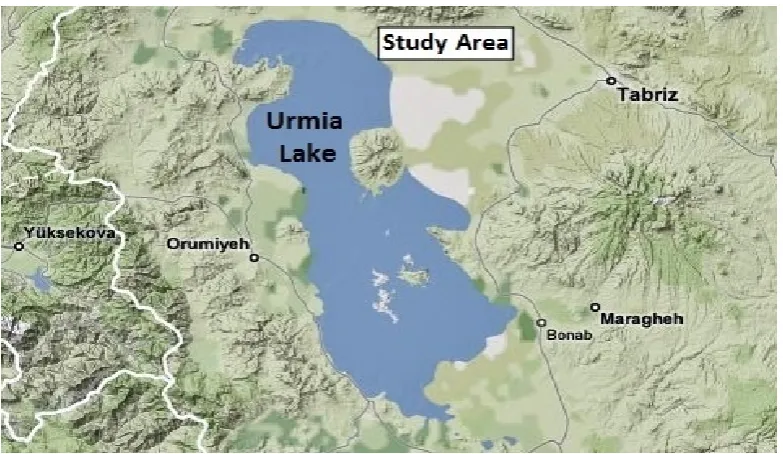
northwest of Iran. It is between 45 26 and 46 2 north latitude and 38 3 and 38 23 east longitude with a cold arid climate. The plain area is about 1,297 km2 and its main river is the Daryanchai. The headwaters of the river are situated at a height of about 2,982m of the Misho Mountain, and it discharges to Urmia Lake. According to statistical results of data from the last 40 years, the average discharge of the Daryanchai River is 0.475 m3/s. The mean daily temperature varies from -19C in January up to 42C in July with a yearly average of 11C and an average annual rainfall of about 250 mm (Nourani and Ejlali, 2012).
As showed by Figure 1, the study area is
a coastal aquifer system. There are about 25 plains around the Urmia Lake basin. The water levels of the lake have a tremendous environmental impact on the groundwater resources from these plains, especially in terms of salinity (Azizi and Abbasi, 2013). A significant population lives in the Urmia Lake basin, whose irrigation economics are strongly dependent on the existing surface, and groundwater resources in the area. Accordingly, the focus of the human population, indiscriminate use, and the recent droughts has reduced the lake’s water level, and seasonal main river. So nowadays, groundwater is a major source of drinking and agricultural water supply.
Fig. 1. Study area in northwest Iran
This study has tried to evaluate the GA-BP and ANN-GA-BP performance models and to provide a comparison of a more optimal model for the estimation of groundwater levels. For this purpose, the data were collected for nine years (from October 2000 to September 2009) with a one month time interval. The data utilized consist of observed groundwater level at 15 piezometers, average discharge of the Daryanchai River, annual time series,
12
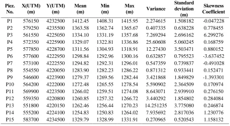
Table 1. Statistical analysis of observed groundwater in 15 piezometers
Skewness Coefficient Standard deviation (m) Variance Max (m) Min (m) Mean (m) Y(UTM) (m) X(UTM) (m) Piez. No. -0.047228 1.508182 2.274615 1415.95 1408.31 1412.45 4232500 576150 P1 0.778455 0.638228 0.407335 1365.67 1362.74 1363.58 4235500 579250 P2 6.299276 2.696162 7.269294 1357.68 1331.19 1334.10 4225050 561550 P3 0.168759 5.060245 25.60608 1336.86 1322.81 1329.07 4225900 572350 P4 0.880152 3.503471 12.27430 1318.91 1304.93 1311.56 4228700 577850 P5 -3.637452 0.795523 0.632857 1300.16 1292.96 1298.84 4222950 577600 P6 -0.491028 0.739837 0.547359 1296.01 1292.31 1294.82 4222550 573100 P7 0.152471 0.933441 0.871312 1286.22 1282.23 1283.90 4220050 554550 P8 -1.393301 1.849829 3.421868 1282.44 1269.56 1279.37 4223900 546600 P9 0.170974 2.364509 5.590902 1278.54 1265.55 1272.48 4222000 564200 P10 0.276150 2.939910 8.643071 1274.08 1259.51 1266.02 4223500 569900 P11 0.284084 1.854802 3.440292 1266.72 1257.32 1260.85 4220800 559350 P12 0.246874 3.775080 14.251235 1270.23 1256.44 1262.46 4220150 551800 P13 1.230776 2.817036 7.935692 1264.02 1250.83 1254.83 4224100 555200 P14 1.158132 0.520543 0.270965 1331.91 1328.99 1329.79 4234500 583700 P15
Fig. 2. Piezometer positions in Shabestar Plain
MARETIALS & METHODS Artificial neural network (ANN)
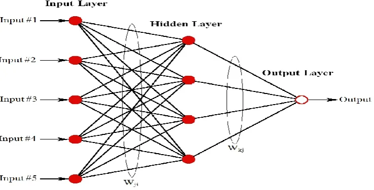
Neural Networks basically comprise interconnected simulated neurons. In hydrological engineering applications to date, the most widely used network is the Feed-Forward Neural Network (FF-NN).
13
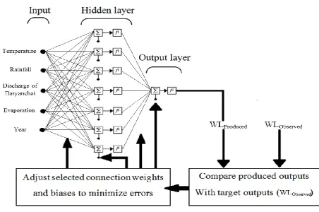
The FF-NN typically consists of three layers, including input, hidden and output layers as depicted in Figure 3. It is possible to have more than one hidden layer but a single layer is sufficient to approximate any function to a desired degree of accuracy (Hornik et al., 1989). The number of neurons in the input and output layers are normally determined by the special problem. Furthermore, for most cases to date, the best way to determine the optimal number of neurons in the hidden layer is done by systemic trial and error. In fact, the inputs are fed through the input layer and, after being multiplied by synaptic weights, are delivered to the hidden layer. In the hidden neurons, the weighted sum of inputs is transformed by a nonlinear activation function, which is usually chosen as the logistic or the hyperbolic tangent. The same process takes place in each of the following hidden layers, until
the outcomes reach the output neuron. Meanwhile, the linear activation function is most commonly applied to the output layer (Triana et al., 2010).
Back-propagation (BP) algorithms are the most popular training algorithms that are widely used due to their simplicity and the application for training FF-NN (Kulluk, 2013). In FF-BP networks, which are considered in this study, output error is reported back, and in this way, a more desirable output is acquired through updating the weighting coefficients matrix. This action is carried out until the error between the target data and output data derived from the weighting matrix is insignificant and consequently the value of the objective function is minimized (Fig.4). For further details on FF-NNs, the reader is referred to the bibliography (ASCE Task Committee on Application of Artificial Neural Networks in Hydrology, 2000).
Fig. 3. Typical Feed-Forward Neural Networks
14 Hybrid genetic algorithm-back propagation (hybrid GA-BP)
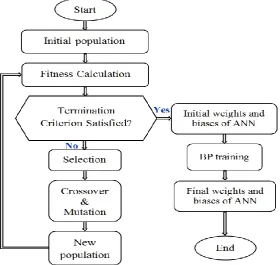
In order to avoid local optimum, the ANN learning process for the hybrid GA-BP model (Liang et al., 2000) consists of two stages: in the first stage, GA is employed to
search for the optima or approximate optimal connection weights and biases for the network. Then in the second stage, the back-propagation training algorithm is used to adjust the final weights and biases (Fig.5).
Fig. 5. GA-BP flow chart
GA is the most well-known evolutionary algorithm, which was introduced by John Holland and his colleague in the 1960s. The study of Jong and Goldberg et al. made significant progress in theoretical study as well as practical applications (Goldberg, 1989). This algorithm has an iterative progress, which begins the search with a random initial solution. In the hybrid GA-BP model, the ANN weights and biases are initialized as genes of chromosomes, and then for searching for the global optimum, three operators (selection, crossover,
and mutation) are used to generate the next
population. GA is stopped when the stopping criteria (e.g., number of generation, stall generation, time limit and so on) is met. After that, this procedure is completed by applying a BP training
algorithm on GA established initial connection weights and biases (Fig.5).
RESULTS & DISCUSSION
In this study, the hybrid GA-BP model is designed in comparison with the ANN-BP model for estimation of groundwater levels. For this purpose, the weights adjustment is done through minimizing the objective function, which is normally defined as a root mean squared error (RMSE), which calculates according to Equation 1.
N
observed predicted i 1 1
RMSE (WL WL )
N
(1)In this equation, RMSE is the root mean squared error, N is the number of training samples, WLobserved is the amount of
15
piezometer, and WLpredicted is the predicted
groundwater level using the GA-BP or ANN-BP model.
As has been explained, the utilized dataset was acquired for October 2000 to September 2009 including Rainfall (mm/month), average discharge of the Daryanchai River (m3/s), temperature (C), evaporation (mm/month), and annual time series (year), which was defined as the external inputs for determining groundwater fluctuations from 15 piezometers. According to recent researches (Coulibaly et al., 2001a; Lallahem et al., 2005; Nourani et al., 2008) effective factors in the fluctuation of groundwater levels include temperature, rainfall and average discharge of the basin. However, typical hydrology and hydrogeology of every basin are different. In the coastal aquifer of the Shabestar Plain, groundwater levels decreased in all piezometers. Undoubtedly, evaporation also has an important role in these decreases. So, in this case study the evaporation data were added to the input layer. Furthermore, in another case study, the evaporation factor is used for the estimation of groundwater levels in another coastal aquifer located in Italy (Taormina et al., 2012). These four input data (temperature, rainfall, average discharge and evaporation) reflect monthly fluctuations in the groundwater level since piezometer groundwater levels decrease with a constant gradient annually, annual time series are also included in the present study. Rainfall values ranged from 3 to 110.2 mm/month (average 20.39), average discharge value from 0.03 to
2.658 m3/s (average 0.41), temperature value from -6.7 to 27C (average 13.41) and evaporation value from 0 to 265.9 mm/month (average 87.39).
For better assessment of the results, all input and output data were normalized using the method introduced by Larose in data mining and statistical analysis (Larose, 2005). Normalization is performed in the typical range of 0 (L) and 1 (H) by using
the maximum and minimum values according to Equations 2-4.
*
i
X mX b (2)
H L
m
Max ( X ) Min( X )
(3)
Max ( X ) L Min( X ) H
b
Max ( X ) Min( X )
(4)
where, X* are the normalized and Xi are
main variables.
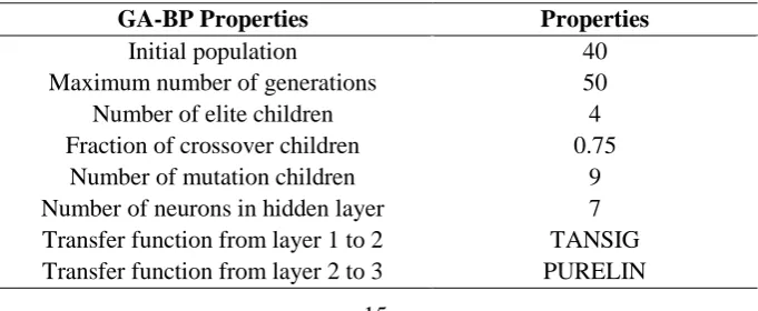
Table 2 represents the parameters that were used in construction of the GA-BP model. Structure of the ANN-BP model designed (5:7:1) for both models consists of three layers, including the input layer, hidden layer and output layer, as shown in Figure 6. Architecture of the feed forward BP neural network consists of five input variables, seven hidden neurons with hyperbolic tangent function and one output variable with a linear activation function, transform the sum of all the weighted inputs into an output signal. By using a trial and error method it was realized that a structure with seven neurons in the hidden layer (5:7:1structure) gives the best results.
Table 2. Parameters used in the construction of the GA-BP model
Properties GA-BP Properties
40 Initial population
50 Maximum number of generations
4 elite children
Number of
0.75 Fraction of crossover children
9 Number of mutation children
7 Number of neurons in hidden layer
TANSIG Transfer function from layer 1 to 2
16
Fig. 6. Typical Architecture of feed forward BP neural network with seven neurons in the hidden layer (Hosseini, 2013); by comparing produced groundwater level (WLProduced) and observed groundwater level (WLObserved) during the training phase, errors propagate backward to the connections in the previous layers.
To make an appropriate comparison between the different intelligent optimization methods the same set of input/output data and training, testing and validation data were used. Meanwhile, the same parameter settings for the individual and hybrid models were used. The total dataset includes 84 training data for each piezometer (October 2000 to September 2007), 12 testing data (October 2007 to September 2008) and 12 validation data (October 2008 to September 2009) for evaluating its accuracy. RMSE and correlation coefficient (R2) between the observed and estimated data were calculated as criteria to evaluate their accuracy.
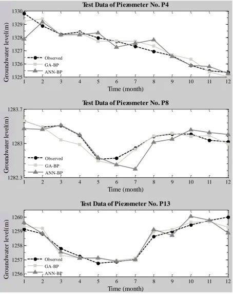
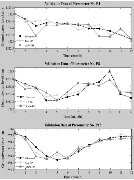
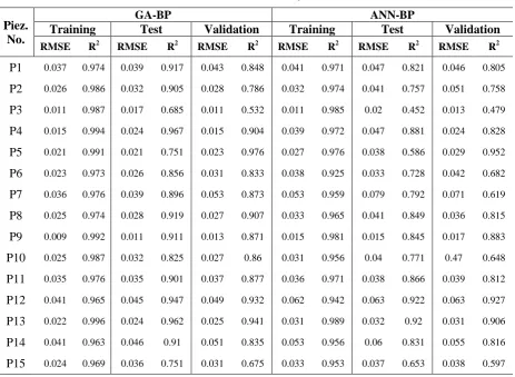
All results of the training and test stage for each model (GA-BP and ANN-BP models) are shown in Table 3. It can be observed that the performance of GA-BP model is much better than that of the ANN-BP model in training, testing and validation data. According to Table 3, the GA-BP
model has the best performance in the training step, providing the best results for test data. Average RMSE and R2 between observed and estimated data using the GA-BP model in training data from 15 piezometers are 0.026 and 0.98, respectively. These amounts for test data are calculated 0.03 and 0.873, and 0.049 and 0.843, respectively, for the validation set. Furthermore, average RMSE and average R2 between observed and predicted groundwater level using the ANN-BP model are 0.036 and 0.965, respectively, in training data, and 0.042 and 0.778, respectively, in test data, as well as 0.068 and 0.768 in the validation data.
17
data by using two intelligent models for testing data. The results clearly show that the GA-BP model is more successful among the individual models designed
(ANN-BP) in this study. This model is faster than GA stochastic models. So, the GA-BP model can be of high prominence in the estimation of groundwater levels.
1 2 3 4 5 6 7 8 9 10 11 12
1325 1326 1327 1328 1329 1330
Time (month)
G
o
u
n
d
w
a
te
r
le
v
e
l
(m
)
Test Data of Piezometer No. P4
1 2 3 4 5 6 7 8 9 10 11 12
1282.3 1283 1283.7
Time (month)
G
ro
u
n
d
w
a
te
r
le
v
e
l
(m
)
Test Data of Piezometer No. P8
1 2 3 4 5 6 7 8 9 10 11 12
1256 1257 1258 1259 1260
Time (month)
G
o
u
n
d
w
a
te
r
le
v
e
l
(m
)
Test Data of Piezometer No. P13
Observed GA-BP ANN-BP Observed GA-BP ANN-BP Observed GA-BP ANN-BP
Fig. 7. Graphical comparison of estimated versus observed groundwater level at selected piezometers using GA-BP and ANN-GA-BP in test stage
Groun
dwat
er level(
m)
Groundwat
er level(
m)
G
ro
u
n
d
w
at
er
l
ev
el
(m
18
1 2 3 4 5 6 7 8 9 10 11 12
1322.5 1323 1323.5 1324 1324.5 1325 1325.5
Time (month)
G
ro
u
n
d
w
a
te
r
le
v
e
l
(m
)
Validation Data of Piezometer No. P4
1 2 3 4 5 6 7 8 9 10 11 12
1255.3 1256.1 1256.9 1257.7 1258.5 1259.3 1260
Time (month)
G
ro
u
n
d
w
a
te
r
le
v
e
l
(m
)
Validation Data of Piezometer No. P13
ObservedGA-BP
ANN-BP
1 2 3 4 5 6 7 8 9 10 11 12
1282 1282.2 1282.4 1282.6 1282.8 1283
Time (month)
G
ro
u
n
d
w
a
te
r
le
v
e
l
(m
)
Validation Data of Piezometer No. P8
Observed
GA-BP
ANN-BP
Observed
GA-BP
ANN-BP
19
Table 3. The results of models for estimation of normal groundwater levels
ANN-BP GA-BP
Piez.
No. Training Test Validation Training Test Validation R2 RMSE R2 RMSE R2 RMSE R2 RMSE R2 RMSE R2 RMSE 0.805 0.046 0.821 0.047 0.971 0.041 0.848 0.043 0.917 0.039 0.974 0.037 P1 0.758 0.051 0.757 0.041 0.974 0.032 0.786 0.028 0.905 0.032 0.986 0.026 P2 0.479 0.013 0.452 0.02 0.985 0.011 0.532 0.011 0.685 0.017 0.987 0.011 P3 0.828 0.024 0.881 0.047 0.972 0.039 0.904 0.015 0.967 0.024 0.994 0.015 P4 0.952 0.029 0.586 0.038 0.976 0.027 0.976 0.023 0.751 0.021 0.991 0.021 P5 0.682 0.042 0.728 0.033 0.925 0.038 0.833 0.031 0.856 0.026 0.973 0.023 P6 0.619 0.071 0.792 0.079 0.959 0.053 0.873 0.053 0.896 0.039 0.976 0.036 P7 0.815 0.036 0.849 0.041 0.965 0.033 0.907 0.027 0.919 0.028 0.974 0.025 P8 0.883 0.017 0.845 0.015 0.981 0.015 0.871 0.013 0.911 0.011 0.992 0.009 P9 0.648 0.47 0.771 0.04 0.956 0.031 0.86 0.027 0.825 0.032 0.987 0.025 P10 0.812 0.039 0.866 0.038 0.971 0.036 0.877 0.037 0.901 0.035 0.976 0.035 P11 0.927 0.063 0.922 0.063 0.942 0.062 0.932 0.049 0.947 0.045 0.965 0.041 P12 0.906 0.031 0.92 0.032 0.989 0.031 0.941 0.025 0.962 0.024 0.996 0.022 P13 0.816 0.055 0.831 0.06 0.956 0.053 0.835 0.051 0.91 0.046 0.963 0.041 P14 0.597 0.038 0.653 0.037 0.953 0.033 0.675 0.031 0.751 0.036 0.969 0.024 P15 CONCLUSION
In this study, the GA-BP and ANN-BP models are designed to estimate groundwater levels in the Shabestar Plain. The nine years of monthly average data including rainfall, temperature, river discharge, annual time series and evaporation criteria, were used as inputs and groundwater level data were considered as output of the models. Results of this study showed that the GA-BP model has better performance than each model individually (GA and ANN-BP models). Results of the simulation with the GA-BP and the ANN-BP models for all piezometers show that average RMSE for testing data are 0.03 and 0.042, respectively. Data for the validation stage are 0.049 and 0.068, respectively. Furthermore, average R2 of the testing and validation set was 0.873 and 0.843 for the
GA-BP model and 0.778 and 0.768 for the ANN-BP model, respectively. The findings of this research demonstrate that employing a genetic algorithm to initialize neural network connection weights in complex space avoids the risk of becoming stuck in local minima. Therefore, in water resources management projects, it can prevent high costs and time wasting for drilling more piezometers. It is expected that the GA-BP model is capable of identifying groundwater levels in other coastal aquifers.
REFERENCES
ASCE Task Committee on Application of Artificial Neural Networks in Hydrology, (2000). Artificial neural networks in hydrology, parts I and II. J. Hydrol. Eng. 5(2), 115-137.
20 Drying Lake Urmia. (Paper presented at 3rd Climate Change Technology Conference, Montreal)
Belew, R. K., McInerney, J., and Schraudolph, N. N. (1991). Evolving networks: using the genetic algorithm with connectionist learning. (In C.G. Langton (Eds.) Artificial Life II. (pp. 511-547) USA: Addison-Wesley)
Chau, K. W. (2007). Application of a PSO-based neural network in analysis of outcomes of construction claims. Autom. Constr., 16(5), 642– 646.
Coulibaly, P., Anctil, F., Aravena, R., and Bobee, B. (2001a). Artificial neural network modeling of water table depth fluctuation. Water Resour. Res., 37(4), 885-896.
Coulibaly, P., Anctil, F., and Bobee, B. (2001b). Multivariate reservoir inflow forecasting using temporal neural networks. J. Hydrol. Eng., 65(9-10), 367-376.
Coulibaly, P., Bobee, B., and Anctil, F. (2001c). Improving extreme hydrologic events forecasting using a new criterion for artificial neural network selection. Hydrol. Process., 15(8), 1533-1536.
Daliakopoulos, I., Coulibaly, P., and Tsanis, I. K. (2005). Groundwater level forecasting using artificial neural networks. J. Hydrol., 309, 229-240.
Dogan, A., Demirpence, H., and Cobaner, M. (2008). Prediction of groundwater levels from lake levels and climate data using ANN approach. Water SA., 34, 199-205.
Goldberg, D. E. (1989). Genetic Algorithm in search, Optimization and Machine Learning. First Ed., (New York: Addison-Wesley Professional)
Hornik, K., Stinchcombe, M., White, H., (1989). Multilayer feed-forward networks are universal approximators. Neural Networks, 2, 359-366.
Hosseini, Z. (2013). Synthesis of geochemical log from petrophysical data using Ant Colony Optimization in the Ahwaz oilfield. (M.S. thesis, Department of Geology, Faculty of Natural Science, University of Tabriz)
Jalalkamali, A., and Jalalkamali, N. (2011). Groundwater modeling using hybrid of artificial neural network with genetic algorithm. Afr. J. Agricul. Res., 6(26), 5775-5784.
Kulluk, S. (2013). A novel hybrid algorithm combining hunting search with harmony search algorithm for training neural networks. J. Oper. Res. Soc., 64(5), 748-761.
Lallahem, S., and Mania, J. (2003a). Evaluation and forecasting of daily groundwater inflow in a small
chalky watershed. Hydrol. Process., 17(8), 1561-1577.
Lallahem, S., and Mania, J. (2003b). A non-linear rainfall-runoff model using neural network technique: Example in fractured porous media. Math. Comput. Model., 37(9-10), 1047-1061.
Lallahem, S., Mania, J., Hani, A., and Najjar, Y. (2005). On the use of neural networks to evaluate groundwater levels in fractured media. J. Hydrol. Eng., 307, 92-111.
Larose D. T. (2005). Discovering knowledge in data: an introduction to data mining. First Ed., (New Jersey: John Wiley & Sons Inc.)
Liang, H., Lin, Z., and McCallum, R. W. (2000). Application of combined genetic algorithms with cascade correlation to diagnosis of delayed gastric emptying from electrogastrograms, Medical Eng. Phys., 22, 229-234.
Maier, H. R., and Dandy, G. C. (2000). Neural networks for the prediction and forecasting of water resources variables: a review of modeling issues and applications. Environ. Modell. Softw., 15(1), 101-124.
Maier, H. R., Jain, A., Dandy, G. C., and Sudheer, K. P. (2010). Methods used for the development of neural networks for the prediction of water resource variables in river systems: current status and future directions. Environ. Modell. Softw., 25(8), 891-909.
Montana, D. J., (1995). Neural network weight selection using genetic algorithms. (In S. Goonatilake and S. Khebbal (Eds.) Intelligent Hybrid Systems (pp. 85-104) New York: John Wiley & Sons)
Moosavi, V., Vafakhah, M., Shirmohammadi, B., and Behnia, N. (2013). A Wavelet-ANFIS Hybrid Model for Groundwater Level Forecasting for Different Prediction Periods. Water Resour. Manag., 27(5), 1301-1321.
Nakhaei, M., and Saberi Naser, A. (2012). A combined Wavelet-Artificial Neural Network model and its application to the prediction of groundwater level fluctuations. J. Geope., 2(2), 77-91.
Nourani, V., Moghaddam, A. A., and Nadiri, A. (2008). An ANN-based model for spatiotemporal groundwater level forecasting. Hydrol. Process., 22, 5054-5066.
21 Nourani, V., and Ejlali, R. G. (2012). Quantity and Quality Modeling of Groundwater by Conjugation of ANN and Co-Kriging Approaches. (In P. Nayak, (Ed.), Water Resour.Manag Modeling, E-Publishing, InTech. pp. 287–310).
Sreekanth, P. D., Geethanjali, N., Sreedevi, P. D., Ahmad, S., Ravi Kumar, N., and Kamala Jayanthi, P. D. (2009). Forecasting groundwater level using artificial neural networks. Curr. Sci. India, 96(7), 933-939.
Taormina, R., Chau, K., and Sethi, R. (2012). Artificial Neural Network simulation of hourly
groundwater levels in a coastal aquifer system of the Venice lagoon. Eng. Appl. Artif. Intell., 25(8), 1670-1676.
Triana, E., Labadie, J.W., Gates, T.K., and Anderson, C.W. (2010). Neural network approach to stream-aquifer modeling for improved river basin management. J. Hydrol., 391, 235-247.