www.geosci-model-dev.net/7/2717/2014/ doi:10.5194/gmd-7-2717-2014
© Author(s) 2014. CC Attribution 3.0 License.
Verification of a non-hydrostatic dynamical core using the horizontal
spectral element method and vertical finite difference method:
2-D aspects
S.-J. Choi1, F. X. Giraldo2, J. Kim1, and S. Shin1
1Korea Institute of Atmospheric Prediction Systems, Seoul, Korea 2Naval Postgraduate School, Monterey, USA
Correspondence to: S.-J. Choi ([email protected])
Received: 23 May 2014 – Published in Geosci. Model Dev. Discuss.: 10 June 2014 Revised: 2 October 2014 – Accepted: 7 October 2014 – Published: 19 November 2014
Abstract. The non-hydrostatic (NH) compressible Euler equations for dry atmosphere were solved in a simplified two-dimensional (2-D) slice framework employing a spec-tral element method (SEM) for the horizontal discretiza-tion and a finite difference method (FDM) for the ver-tical discretization. By using horizontal SEM, which de-composes the physical domain into smaller pieces with a small communication stencil, a high level of scalability can be achieved. By using vertical FDM, an easy method for coupling the dynamics and existing physics packages can be provided. The SEM uses high-order nodal ba-sis functions associated with Lagrange polynomials based on Gauss–Lobatto–Legendre (GLL) quadrature points. The FDM employs a third-order upwind-biased scheme for the vertical flux terms and a centered finite difference scheme for the vertical derivative and integral terms. For temporal in-tegration, a time-split, third-order Runge–Kutta (RK3) inte-gration technique was applied. The Euler equations that were used here are in flux form based on the hydrostatic pressure vertical coordinate. The equations are the same as those used in the Weather Research and Forecasting (WRF) model, but a hybrid sigma–pressure vertical coordinate was implemented in this model.
We validated the model by conducting the widely used standard tests: linear hydrostatic mountain wave, tracer ad-vection, and gravity wave over the Schär-type mountain, as well as density current, inertia–gravity wave, and rising ther-mal bubble. The results from these tests demonstrated that the model using the horizontal SEM and the vertical FDM is accurate and robust provided sufficient diffusion is applied.
The results with various horizontal resolutions also showed convergence of second-order accuracy due to the accuracy of the time integration scheme and that of the vertical direction, although high-order basis functions were used in the hori-zontal. By using the 2-D slice model, we effectively showed that the combined spatial discretization method of the spec-tral element and finite difference methods in the horizontal and vertical directions, respectively, offers a viable method for development of an NH dynamical core.
1 Introduction
and Loft, 2005) and the scalable spectral element Eulerian at-mospheric model (SEE-AM) (Giraldo and Rosmond, 2004). These models consider the primitive hydrostatic equations on global grids, such as a cubed sphere tiled with quadrilateral elements using SEM in the horizontal discretization and the finite difference method (FDM) in the vertical. The robust-ness of SEM has been illustrated through three-dimensional dry dynamical test cases (Giraldo and Rosmond, 2004; Gi-raldo, 2005; Thomas and Loft, 2005; Taylor et al., 2007; Lau-ritzen et al., 2010).
The ultimate objective of our study is to build a 3-D non-hydrostatic (NH) model based on the compressible Navier–Stokes equations using SEM in the horizontal dis-cretization and FDM in the vertical. Because testing a 3-D NH model requires a large amount of computing resources, studying the feasibility of our approach in 2-D is an attrac-tive alternaattrac-tive to the development of a fully 3-D model. This is the case because a 2-D slice model can effectively test the practical issues resulting from the vertical discretization and time integration prior to construction of a full 3-D model. Al-though we could discretize the vertical direction using SEM (as proposed in Kelly and Giraldo, 2012, and Giraldo et al., 2013), we chose to use a finite difference method for dis-cretization in the vertical direction because it provides an easy way to couple the dynamics and existing physics pack-ages.
For this objective, we developed a dry 2-D NH compress-ible Euler model based on SEM along the x direction and FDM along thezdirection, which we hereafter refer to as the 2-D NH model. We adopted the governing equation formula-tion proposed by Skamarock and Klemp (2008) (SK08 here-after), which is used in the Weather Research and Forecast-ing (WRF) model. The Euler equations are in flux form based on the hydrostatic pressure vertical coordinate. In SK08, the terrain-following sigma–pressure coordinate is used, but we here employed a hybrid sigma–pressure vertical coordinate. Park et al. (2013) (PK13 hereafter) provided a clue for the equation set in the hybrid sigma–pressure in their Appendix, in which the hybrid sigma–pressure coordinate is applied to the hydrostatic primitive equations and can be modified ex-actly to the sigma–pressure coordinate at the level of the ac-tual coding implementation. We also built the 2-D NH model using a time-split, third-order Runge–Kutta (RK3) for the time discretization, which has been shown to be effective in the WRF model. We kept the temporal discretization of the model as similar as possible to the WRF model in order to more directly discern the differences related to the discrete spatial operators between the two models. This provides ro-bust tools for development and verification of the 2-D NH model.
In this paper, we demonstrate the feasibility of the 2-D NH model by conducting conventional benchmark test cases and by focusing on the description of the numerical scheme for the spatial discretization. We verify the 2-D NH by analyz-ing six test cases: inertia–gravity wave, risanalyz-ing thermal
bub-ble, density current wave, linear hydrostatic mountain wave, and tracer advection and gravity wave over the Schär-type mountain.
The organization of this paper is as follows. In the next section, we describe the governing equations with definitions of the prognostic and diagnostic variables used in our model. In Sect. 3, we explain the temporal and spatial discretiza-tion including the spectral element formuladiscretiza-tion. In Sect. 4, we present the results of the 2-D NH model using all four test cases, and finally, in Sect. 5, we summarize the paper and propose future directions.
2 Governing equations
We adopted the formulation of the governing-equation set of SK08. Here, we implemented the hybrid sigma–pressure coordinate introduced in PK13, which only considers the hy-drostatic primitive equation. The hybrid sigma pressure co-ordinate is defined withη∈[0,1] as
pd=B(η) (ps−pt)+[η−B(η)](p0−pt)+pt, (1) wherepd is the hydrostatic pressure of dry air;B(η)is the relative weighting of the terrain-following coordinate versus the normalized pressure coordinate; andps,pt, andp0 are the hydrostatic surface pressure of dry air, the top-level pres-sure, and a reference sea level prespres-sure, respectively. A more detailed description of the hybrid sigma–pressure coordinate can be found in the Appendix of PK13. The definition of the flux variables are
(VH, W, , 2)=µd×(vH, w,η, θ ) ,˙ (2) wherevH=(u, v)andw are the velocities in the horizon-tal and vertical directions, respectively; η˙≡dη
dt is the η
-coordinate (contravariant) vertical velocity;θis the potential temperature; andµdis the mass of the dry air in the layers, defined as
µd(x, y, η, t )=
∂pd ∂η =
∂B(η)
∂η (ps−pt)+
1−∂B(η) ∂η
(p0−pt) . (3) The flux-form Euler equations for dry atmosphere to be recast using perturbation variables are expressed as
∂VH
∂t = −µd ∇ηφ 0+
αd∇ηp0+αd0∇ηp¯
−
∂p0 ∂η −µ
0 d
∇ηφ− ∇η·(VH⊗vH)−
∂ (vH)
∂η +FVH, (4)
∂W ∂t =g
∂p0 ∂η −µ
0 d
− ∇η·(VHw)− ∂ (w)
∂η +FW, (5) ∂µ0d
∂t = ∂ ∂t
∂p0 d ∂η
=∂B(η) ∂η
∂ps0
∂t = −∇η·VH− ∂ ∂η, (6) ∂φ0
∂t = − 1 µd
VH· ∇ηφ+ ∂φ ∂η−gW
∂2
∂t = −∇η·(VHθ )− ∂ (θ )
∂η , (8)
whereφis the geopotential;αdis the inverse density for dry air; andFVH andFWrepresent forcing terms of Coriolis and curvature, which we ignore for simplicity. In Eqs. (4)–(8), the governing equations are described with perturbation vari-ables, such asp= ¯p(z)¯ +p0,φ= ¯φ (z)¯ +φ0,αd= ¯αd(z)¯ +α0d, and ps= ¯ps(x, y)+p0s, where the variables denoted by an overbar are the reference state variables that satisfy hydro-static balance.
For completeness, the diagnostic relation foris given by integrating Eq. (6) vertically from the surface (η=1)to the material surface: = − η Z 1 ∂B(η) ∂η
∂p0s
∂t + ∇η·VH
dη, (9)
where ∂p
0 s
∂t is obtained by integrating Eq. (6) vertically from
the surface (η=1) to the top (η=0) using a no-flux bound-ary condition, such as |η=0 or 1=0.∂p
0 s
∂t is defined as ∂p0s
∂t = − η=1 Z
η=0
(∇ ·VH)dη. (10)
The above equation allows forps0to be evolved forward in time, where we then computeµ0ddirectly from Eq. (5). The diagnostic relation for the dry inverse density is given as
∂φ0
∂η = − ¯µdα 0
d−αdµ0d, (11)
and the full pressure for dry atmosphere is
p=p0
R
dθ p0αd
cp/cv
. (12)
This concludes the description of the governing equations used in our model; in the next section, we describe the dis-cretization of the continuous form of the governing equations that are used in our model.
3 Discretization
3.1 Spatial discretization 3.1.1 Horizontal direction
For a givenηlevel, we discretized the horizontal operators using SEM. Therefore, in the 2-D (x−z) slice framework, we focus on the SEM discrete gradient operator for 1-D (x). In SEM, we approximate the solution in non-overlapping el-ementseas
q(x, t )=
N+1 X
i=1
ψi(x)qN(xi, t ), (13)
wherexi represents theN+1 grid points that correspond to
the Gauss–Lobatto–Legendre (GLL) points andψi(x)are the Nth-order Lagrange polynomials based on the GLL points. It is worth noting that theψi have the cardinal property, i.e.,
they can be represented as Kronecker delta functions where ψi are zero at all nodal points exceptxi.
The GLL pointsξi in a reference coordinate systemξ ∈
[−1,+1] and the associated quadrature weightsω(ξi), ω(ξi)=
2 N (N+1)
1
PN(ξi) 2
, (14)
are introduced for the Gaussian quadrature:
Z
e qde=
+1 Z
−1
q(ξ )|J (ξ )|dξ≈
N X
i=0
ω(ξi)q(ξi)|J (ξi)|, (15)
where PN(ξ ) are the Nth-order Legendre polynomials, J=∂x
∂ξ is the transformation Jacobian, and
erepresents the non-overlapping elements.
We now introduce the polynomial expansions into our governing equations in the form of
∂q
∂t = −F (q), (16)
multiply by the basis functionψi as a test function, and
in-tegrate to yield a system of ordinary differential equations, such as
Mj ie dqi dt = −
Z
e ψjF
N+1 X
i=1 ψi(ξ )qi
!
dξ, (17)
wherei=1,2,· · ·, N+1,Mj ie is the element-based mass ma-trix given as
Mj ie =
Z
e
ψjψidξ=ωj Jj
δj i. (18)
The right-hand sides of Eqs. (17) and (18) are evaluated using the Gaussian quadrature of Eq. (15). It is noted that using GLL points for both interpolation and integration re-sults in a diagonal mass matrixMj ie, which means that the inversion of the mass matrix is trivial.
The horizontal derivatives included in the right-hand side of Eq. (17) are evaluated using the analytic derivatives of the basis functions as follows:
∂q ∂x= ∂q ∂ξ ∂ξ ∂x = ∂ ∂ξ
"N+1
X
i=1
ψi(ξ )qi #
∂ξ ∂x =
"N+1
X
i=1
∂ψi
∂ξ qi
# 1
3.1.2 Vertical direction
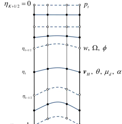
Using a Lorenz staggering, the variablesVH,2,µ,α, andp are at layer midpoints denoted byk=1,2, . . ., K, whereKis the total number of layers, and the variablesW,, andφare at layer interfaces defined byk+1
2,k=0,1, . . ., K, so that ηK+1/2=ηtopandη1/2=ηBottom=1. Figure 1 describes the grid points and the allocation of the variables. Here, we eval-uate the vertical advection terms∂(vH)
∂η ,
∂(w) ∂η ,and
∂(θ ) ∂η
and vertical derivative terms ∂p∂η0 and∂φ∂η. The former is discretized using the third-order upwind-biased discretiza-tion in Hundsdorfer et al. (1995), which is given as
∂f ∂η k
=fk−2−8fk−1+8fk+1−fk+2 121η
+sign()fk−2−4fk−1+6fk−4fk+1+fk+2
121η , (20)
where f corresponds to the flux, such as vH, and 1η=ηk+1/2−ηk−1/2is the thickness of the layer. The latter is discretized by the centered finite difference, which is given as ∂g η k
=gk+1/2−gk−1/2
1η , (21)
wheregcorresponds to the variablesp0andϕ. Likewise, the vertical discretization integration rules for the calculations of Eqs. (9) and (10) follow the finite difference naturally as
Z
qdη=X
k
qk+1/2(ηk+1−ηk) . (22)
3.1.3 Explicit diffusion
In addition to the governing equations, a viscous term might be needed to conduct some tests. The viscosity used here is an explicit Laplacian (∇2)diffusion operator on coordi-nate surfaces. In order to implement the Laplacian operator f =νh ∂
2
∂x2(µda)for a model flux variableµda, we multiply by the basis functionψas a test function and integrate using the divergence theorem to yield the weak form equation Z
e
ψfde=Kh
Z
0e ψ ∂
∂x(µda)d0 e−
Z
e ∂ ∂xψ·
∂
∂x(µda) d e
, (23) whereνhdenotes the eddy viscosity coefficient and the term
with0eis a boundary integral that accounts for internal faces (neighboring elements share faces). Because we used the pe-riodic boundary condition in this study, the boundary integral term of the right-hand side can be ignored in all elements, which allows us to rewrite the equations as
Z
e
ψfde= −νh Z
e ∂ψ
∂x ∂
∂x(µda)d
e. (24)
cv
cv
cv
cv
cv
1/ 20
η
K+=
1/ 2
1
η
=
1/ 2 ηk+
ηk
1/ 2 ηk−
, , , ,
θ µ α
H d
p
v
, ,
Ω
φ
w
sp
tp
Figure 1. Grid points of columns within an element having four
GLL points. The hybrid sigma–pressure coordinates are illustrated, and the closed (open) circles on the solid (dashed) line indicate the location of the variables at layer midpoints (interfaces).
After introducing the polynomial expansions, such as a(x, t )=
N+1 P
i=1
ψi(x)aN(xi, t ), the integrals of the above
equation can be approximated using SEM. A description of the Laplacian operator using SEM can also be found in Denis et al. (2011). The vertical Laplacian operator for a model flux variableµdais added to a governing equation as follows:
∂
∂t(µda)=. . .+νvg
2(µ dα)−1
∂ ∂η
(µdα)−1∂ (µda) ∂η
, (25) whereνvdenotes the vertical eddy viscosity coefficient and α is the inverse density. It is noted that the above term is not more thanνv∂
2(µ da)
∂z2 . The vertical derivative term ∂ ∂η is
discretized by the centered finite difference. 3.2 Temporal discretization
acoustic-mode filterings of the forward centering of the vertically im-plicit portion and divergence damping of the horizontal mo-mentum equation are used, which is the same as in the WRF model (Skamarock et al., 2008). It is notable that the time-split RK3 integration scheme is third-order accurate for lin-ear equations and second-order accurate for nonlinlin-ear equa-tions (SK08).
This technique has been shown to work effectively within numerous non-hydrostatic models, including the WRF model (Skamarock et al., 2008), the Model for Predic-tion Across Scales (MPAS) (Skamarock et al., 2012), and the Non-hydrostatic Icosahedral Atmospheric Model (NICAM) (Satoh et al., 2008). It is also noted that, in the procedure of the time-split RK3 integration, the difference between the approach used in this paper and that in SK08 comes from the vertical coordinate. Since we use the hybrid sigma–pressure coordinate, the equation forp0s(Eq. 6) should be first stepped forward in time using forward–backward differencing on the small time steps, thenµ0dcan be computed directly from the specification of the vertical coordinate in Eq. (9) andcan be obtained from the vertical integration.
4 Test cases
We validated the 2-D NH model with six test cases: linear hy-drostatic mountain-wave, tracer-advection, and gravity-wave tests over Schär Mountain, as well as density current, iner-tia–gravity wave, and rising thermal bubble experiments. The last three cases do not have analytic solutions. Therefore, for the mountain experiments, the numerical results of the 2-D NH model were compared with analytic solutions (Durran and Klemp, 1983; Schär et al., 2002); for the other experi-ments, we compared our results with the results of other pub-lished papers.
It should be mentioned that the horizontal SEM formula-tion is able to utilize arbitrary-order polynomials per element to represent the discrete spatial operators, but in this paper all the results presented use either fifth- or eighth-order polyno-mials. The averaged horizontal grid spacing is defined as
1x¯=
N P
n=1 1xn
N , (26)
where1xn is the internal grid spacing within the element,
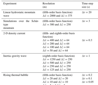
which is regularly spaced in the domain, andNis the number of intervals associated with irregularly spaced GLL quadra-ture points, which is equivalent to the order of the basis poly-nomials. The average vertical grid spacing is defined as in Eq. (26). Below, we use this convention to define the grid resolution. The resolutions and time-step sizes used for all the cases are summarized in Table 1.
4.1 Linear hydrostatic mountain-wave test
We simulated the linear hydrostatic mountawave test in-troduced by Durran and Klemp (1983) (DK83 hereafter) in which the analytic steady-state solution is provided by using a single-peak mountain with uniform zonal wind. To com-pare our results with the analytic and numerical solutions shown in DK83, the 2-D NH was initialized using the same initial conditions and mountain profile as in DK83, and we analyzed our results using the same metrics as DK83.
The mountain profile is given by
h(x)= hm
1+x−xc am
2, (27)
where the half-length of the mountain am is 10 km, the height hm is 1 m, and the prescribed center xc of the pro-file is 0 km. The initial temperature is T0=250 K for an isothermal atmosphere with the uniform zonal wind u¯= 20 m s−1. In the isothermal case, the Brunt–Väisälä fre-quencyN2=gd(lndzθ )¯ ≈ g2
cpT0 yields the potential temperature as
¯ θ=θ0e
g
cpT0z, (28)
which is one of the prognostic variables in our model. The domain is defined as(x, z)∈[−300,300]×[0,30] km2. The bottom boundary uses a no-flux boundary condition, whereas the lateral and top boundaries use sponge layers. The sponged zone is 10 km deep from the top and 50 km wide from the lateral boundaries. Over the sponge-layer zone, the prognostic variables are relaxed to the basic initial hydro-static state. The model is integrated with a grid resolution of 1x¯=2 km using fifth-order basis polynomials per ele-ment and1z¯=375 m for a nondimensional time ofut¯a =60, which corresponds to 8.33 h. Additionally, the model is run without diffusion or viscosity.
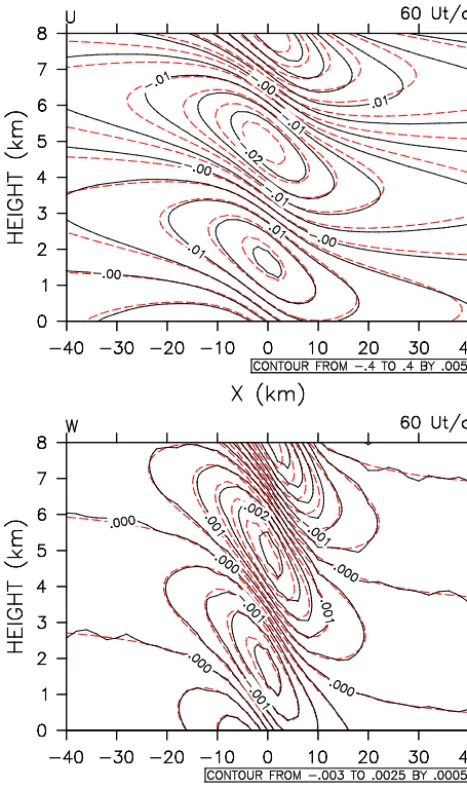
Figure 2 shows the numerical and analytic solutions at steady state for the horizontal and vertical velocities, which agree reasonably well. The vertical velocity fields match very closely, although the extrema in the horizontal veloc-ity field are underestimated by the numerical model. The underestimated extrema in the horizontal velocity were also shown in both models of DK83, which used1x=2 km and 1z=200 m, and in Giraldo and Restelli (2008) (GR08 here-after), which used1x¯=1.2 km and1z¯=240 m with 10th-order basis polynomials. Our result in the horizontal velocity is in good agreement with DK83 and GR08.
Table 1. Summary of the resolutions and time-step sizes used for the tests.
Experiment Resolution (m)
Time-step size (s)
Linear hydrostatic mountain wave
(fifth-order basis function)
1x¯=2000 and1z¯=375
1t=20
Simulations over the Schär-type
mountain
(fifth-order basis function)
1x¯=300 and1z¯=250
1t=3
2-D density current (fifth- and eighth-order basis function)
1x¯=400 and1z¯=64
1x¯=200 and1z¯=64
1x¯=100 and1z¯=64
1x¯=50 and1z¯=64
1t=0.3
Inertia–gravity wave (eighth-order basis function)
1x¯=1250 and1z¯=250
1x¯=500 and1z¯=250
1x¯=250 and1z¯=250
1x¯=125 and1z¯=250
1t=1
Rising thermal bubble (fifth-order basis function)
1x¯=20 and1z¯=20
1x¯=10 and1z¯=10
1x¯=5 and1z¯=5
1t=0.2
1t=0.1
1t=0.05
Durran–Klemp model is based on the FD method in both di-rections, while the Giraldo–Restelli model is based on SEM in both directions. The mountain test shows that the terrain-following vertical coordinate is well suited for the combi-nation of horizontal SEM and vertical FDM for spatial dis-cretization, even though we considered a small mountain.
4.2 Tracer-advection and gravity-wave tests over the Schär-type mountain
In order to verify the feasibility of 2-D NH to treat steep sur-face elevations associated with the vertical terrain-following coordinate, we performed the tracer-advection and gravity-wave experiments introduced by Schär et al. (2002) (SC02 hereafter), in which the mountain is defined by a five-peak mountain chain, over the Schär-type mountain. To compare our results with the numerical solution shown in SC02, the initial conditions and mountain profiles are the same as those of SC02.
For the tracer-advection test, the mountain profile is given by
h(x)=
( h0cos2
π x λ
cos2π x 2a
for|x| ≤a 0 for|x| ≥a
, (29)
whereh0=3 km,a=25 km, andλ=8 km. The prescribed wind profile is given by
u(z)=u0
1 forz2≤z sin2
π
2 z−z1 z2−z1
forz1≤z≤z2 0 forz≤z1,
(30)
whereu0=10 m s−1,z1=4 km, andz2=5 km, and the ini-tial tracer is assigned as
q(x, z)=q0
cos2 π r2 forr≤1
0 else (31)
with r=
" x−x
0 Ax
2
+
z−z 0 Az
2#1/2 ,
where amplitude q0=1, location (x0, z0)=(−50,9)km, and the half-width(Ax, Az)=(25,3)km. Since the domain
is defined as (x, z)∈[−150,150]×[0,25] km2, the tracer is centered directly over the mountain at time 2500 s. The model is integrated with a grid resolution of 1x¯=300 m using fifth-order basis polynomials per element and1z¯= 250 m using 100 levels for 5000 s. The model is run with-out any diffusion, filter, or limiter. It should be noted that the advection equation used in this study is the advective form defined as
∂q ∂t = −
u∂q
∂x+ ˙η ∂q ∂η
31
1
FIG. 2. Steady-state flow of (top) horizontal velocity (m/s) and (bottom) vertical velocity
2
(m/s) over 1-m high mountain at nondimensional time
ut
60
a
=
with a grid resolution of
3
2
x
∆ =
km using 5th-order basis polynomials per element and
∆ =z
375m. The numerical
4
solution is represented by solid lines and the analytic solution is represented by dashed lines.
5
6
Figure 2. Steady-state flow of (top) horizontal velocity (m s−1) and (bottom) vertical velocity (m s−1) over 1 m high mountain at nondi-mensional time ut¯a =60 with a grid resolution of1x¯=2 km using fifth-order basis polynomials per element and1z¯=375 m. The nu-merical solution is represented by solid lines and the analytic solu-tion is represented by dashed lines.
The numerical solutions and the error field are shown in Fig. 4. The figure uses the same contouring interval as in SC02. Even att=2500 s, when the center of the tracer is lo-cated over the center of the mountain, the distribution of the initial tracer is generally maintained (Fig. 4a), which means that 2-D NH using the horizontal spectral element method and vertical finite difference method can produce numeri-cal solutions of good quality in response to the strong ver-tical gradient in the coordinate deformation. It is worth not-ing that the error in Fig. 4b at t=5000 s gives ranges of
−
2.71×10−2,2.35×10−2
, which are substantially small, and that the error is distributed mainly over the mountain where distortion of the computational grid is significant.
32 1
FIG. 3. Vertical flux of horizontal momentum, normalized by its analytic value at several 2
nondimensional times ut
a . M and MH are the momentum flux of the numerical and analytic
3
solutions. 4
5
Figure 3. Vertical flux of horizontal momentum, normalized by its
analytic value at several nondimensional timesut¯a.MandMHare
the momentum flux of the numerical and analytic solutions.
The Schär-type mountain gravity-wave test was initialized in a stratified atmosphere with the Brunt–Väisälä frequency of N=0.01 s−1, the constant mean flow of u¯=10 m s−1, and the initial temperature ofT0=288 K. In the Schär-type mountain gravity wave, the highest mountain peak wash0= 250 m, which is relatively lower than that in the advection test. The mountain profile is given by
h(x)=h0exp
−
x a
2
cos2π x λ
, (33)
wherea=5 km andλ=4 km, and the domain is defined as (x, z)∈[−30,30]×[0,21] km2. The model was integrated with a grid resolution of1x¯=300 m using fifth-order basis polynomials per element and1z¯=250 m using 80 levels for 10 h without any diffusion or viscosity. The bottom boundary had a no-flux boundary condition, while the lateral and top boundaries had sponge layers. The sponged zone was 10 km deep from the top and 5 km wide from the lateral boundaries. Over the sponge layer zone, the prognostic variables were relaxed to the initial state.
33 1
FIG. 4. Tracer advection test over the topography (red line). (a) Advective tracer at time 2
0 (black line), 2500 s (orange), and 5000 s (blue). The contour values are from −1.0 to 1.0 3
with an interval of 0.1. (b) Error at time 5000 s. The contour values are from −0.24 to 0.2 with 4
an interval of 0.01. The numerical solutions were obtained with a grid resolution of 5
300
x
∆ = m using 5th-order basis polynomials per element and ∆ =z 250 m. The sky-blue 6
dashed lines indicate surfaces of constant eta. The zero contour level is omitted. 7
(a)
(b)
Figure 4. Tracer advection test over the topography (red line). (a) Advective tracer at time 0 (black line), 2500 s (orange), and
5000 s (blue). The contour values are from−1.0 to 1.0 with an in-terval of 0.1. (b) Error at time 5000 s. The contour values are from
−0.24 to 0.2 with an interval of 0.01. The numerical solutions were obtained with a grid resolution of1x¯=300 m using fifth-order ba-sis polynomials per element and1z¯=250 m. The sky-blue dashed lines indicate surfaces of constant eta. The zero contour level is omitted.
Table 2. Root-mean-square errors (RMSEs) of the Schär-type
mountain wave after 10 h for 1x¯=300 m using fifth-order poly-nomials per element and1¯z=250 m using 80 levels.
Variable RMSE
u(m s−1) 1.43×10⁻¹
w(m s−1) 3.97×10⁻²
θ(K) 3.77×10⁻²
4.3 2-D density current test
In order to verify the feasibility of 2-D NH to control os-cillations with numerical viscosity and evaluate numerical schemes in 2-D NH, we conducted the density current test suggested by Straka et al. (1993). The density current test is initialized using a cold bubble in a neutrally stratified at-mosphere. When the bubble touches the ground, the density current wave starts to spread symmetrically in the
horizon-34
1
FIG. 5. Steady-state flow of (a) perturbed horizontal velocity (
m s
−1) and (b) vertical
2
velocity (
m s
−1) over Schär Mountain after 10 h with a grid resolution of
∆ =
x
300
m using
3
5th-order basis polynomials per element and
∆ =
z
250
m. The numerical solution is
4
represented by black lines and the analytic solution is represented by red lines. Dashed lines
5
denote negative values. The contour values are from −2.0 to 2.0 with an interval of 0.2 (0.05)
6
for the horizontal velocity (the vertical velocity).
7
8
(a)
(b)
Figure 5. Steady-state flow of (a) perturbed horizontal velocity
(m s−1) and (b) vertical velocity (m s−1) over the Schär-type moun-tain after 10 h with a grid resolution of1x¯=300 m using fifth-order basis polynomials per element and1z¯=250 m. The numeri-cal solution is represented by black lines and the analytic solution is represented by red lines. Dashed lines denote negative values. The contour values are from−2.0 to 2.0 with an interval of 0.2 (0.05) for the horizontal velocity (the vertical velocity).
35 1
FIG. 6. Potential temperature perturbation after 900 s using grid spacing of (a) 2
400
x
∆ = m, (b) ∆ =x 200m, (c) ∆ =x 100m, and (d) ∆ =x 50m, with 5th-order basis 3
polynomials per element for the density current. All simulations use ∆ =z 64m grid spacing. 4
The contour values are from −14.5 to −0.5 with an interval of 1.0. 5
6
(a)
(b)
(c)
(d)
Figure 6. Potential temperature perturbation after 900 s using grid
spacing of (a)1x¯=400 m, (b)1x¯=200 m, (c)1x¯=100 m, and
(d)1x¯=50 m, with fifth-order basis polynomials per element for the density current. All simulations use 1z¯=64 m grid spacing. The contour values are from−14.5 to−0.5 with an interval of 1.0.
For an initial cold bubble, the potential temperature per-turbation is given as
θ0=θc
2 [1+cos(π r)], (34)
whereθc= −15 K andr= r
x−xc
xr 2
+z−zc zr
2
, with the center of the bubble at (xc, zc)=(0,3000)m and the size parameter(xr, zr)=(4000,2000)m. No-flux boundary
con-ditions were used for all boundaries, and the model was integrated for 900 s on the domain [−25 600,25 600]× [0,6400] m2. In this study, the potential temperature per-turbation of θc= −15 K was adopted for comparison with
GR08 and Li et al. (2013). Straka et al. (1993) originally used a−15 K temperature perturbation. The−15 K potential tem-perature corresponds to−13.53 K temperature.
Figure 6 shows the potential temperature perturbation af-ter 900 s for 400, 200, 100, and 50 m grid spacings (1x)¯ using fifth-order basis polynomials per element. All simu-lations used1z¯=64 m grid spacing vertically. As expected, the higher-resolution experiments produced better solutions than the lower-resolution experiments. At the very lowest resolution of 400 m, only two of the three Kelvin–Helmholtz rotors were generated with somewhat coarsened frontal sur-faces. In the experiment with a resolution of 200 m, the three rotors appeared, but the numerical solution still suffered from the coarsening of frontal surfaces. The solutions on grids finer than 100 m converged with the three rotor structures ad-equately simulated. The converged solution was almost iden-tical to other published solutions (e.g., Straka et al., 1993; Skamarock and Klemp, 2008; GR08).
In order to examine the effect of higher order of the ba-sis polynomials than fifth-order, we show profiles of the po-tential temperature perturbation at the height of 1200 m in the simulations using fifth-order polynomials together with the simulations using eighth-order polynomials (Fig. 7). Note that the simulations using eighth-order polynomials have the same number of GLL grid points as the simulations using fifth-order basis polynomials. This was achieved by using a lower number of elements in the eighth-order experiment than in the fifth-order experiment as the number of grid points at a given level becomesne×np, in whichne refers to the number of elements andnpdenotes the polynomial or-der of the elements. It is also noted that we arbitrarily choose eighth-order as the higher order. The results from the high-est grid resolution of the simulations using fifth- and eighth-order polynomials are indistinguishable and well converged, with three minima corresponding to the three rotors, which agree well with other published solutions (Fig. 7a). In addi-tion to the profiles, the front locaaddi-tion (−1 K of potential tem-perature perturbation at the surface) and the extrema of the pressure perturbation and potential temperature perturbation agreed well with each other (Table 3). The numbers in Ta-ble 3 are comparaTa-ble to those of GR08. Although the poten-tial temperature profiles of the simulations using fifth-order polynomials tend to have more fluctuations than those using eighth-order basis polynomials, the simulations do not show a large difference between using eighth-order and fifth-order basis polynomials (Fig. 7b and c).
Table 3. Comparison between fifth- and eighth-order polynomials per element for the density current. The simulation was conducted with a
resolution of1x¯=50 m and1z¯=50 m.
Order of polynomials Front location (km) pmax0 (Pa) pmin0 (Pa) θmax0 θmin0
5th 14.77 630.62 −452.79 0.08 −8.87 8th 14.74 626.91 −456.84 0.08 −8.94
36 1
FIG. 7. Profiles of (a) potential temperature perturbation after 900 s along 1200 m height 2
using grid spacing of ∆ =x 50m with 5th-order (thin solid line) and 8th-order (thick solid 3
line) basis function, (b) difference between various resolution and ∆ =x 50m with 5th-order 4
basis function, (c) difference between various resolution and ∆ =x 50m with 8th-order basis 5
function. 6
7
(a)
(b)
(c)
Figure 7. Profiles of (a) potential temperature perturbation after
900 s along 1200 m height using grid spacing of1x¯=50 m with fifth-order (thin solid line) and eighth-order (thick solid line) basis function, (b) difference between various resolution and1x¯=50 m with fifth-order basis function, and (c) difference between various resolution and1x¯=50 m with eighth-order basis function.
37 1
FIG. 8. Self-convergence test for the density current test; Relative L2 error norms of the 2
potential temperature perturbation θ′ as functions of the space resolution ∆x are shown. The 3
reference solutions for these computations were made with ∆ =x 25 m, ∆ =z 64 m, and 4
0.1 t
∆ = s. The dotted line represents second-order convergence. 5
6
Figure 8. Self-convergence test for the density current test; relative
L2 error norms of the potential temperature perturbationθ0as func-tions of the space resolution1x¯are shown. The reference solutions for these computations were made with1x¯=25 m,1z¯=64 m, and 1t=0.1 s. The dotted line represents second-order conver-gence.
were interpolated to the equidistant grid of 1x=400 and 1z=50 and then used to evaluate errors. Here, we evalu-ated the error by using the relative L2 error defined by
kqsimulationkL2= v u u t R
(qref−qsimulation) 2d R
q 2 refd
, (35)
4.4 Inertia–gravity-wave test
This test examines the evolution of a potential temperature perturbationθ0in a constant mean flow with a stratified atmo-sphere. This initial potential temperature perturbationθ0 radi-ates symmetrically to the left and right in a channel with pe-riodic lateral boundary conditions. The inertia–gravity-wave test introduced by Skamarock and Klemp (1994) (SK94 here-after) serves as a tool to investigate the accuracy for NH dy-namics. We also used this experiment to check the consis-tency of the results at various resolutions. The parameters for the test were the same as those of SK94. The initial state was a constant Brunt–Väisälä frequency ofN=0.01 s−1with a surface potential temperature of θ0=300 K and a uniform zonal wind ofu¯=20 m s−1. In order to trigger the wave, the initial potential temperature perturbationθ0was overlaid the above initial state and is given as
θ0(x, z)=θc
sinπ zz c
1+x−xc ac
2, (36)
whereθc=0.01 K,zc=10 km,xc=100 km, andac=5 km. The domain was defined as (x, z)∈[0,300]×[0,10] km2. We used periodic lateral boundary conditions and no-flux boundary conditions for both the bottom and top boundaries. The simulation was performed for 3000 s with no viscosity.
Figure 9 shows the solution θ0 at the initial time and at time 3000 s with horizontal resolution1x¯=250 m and ver-tical resolution1z¯=250 m. For comparison, the figure uses the same contouring interval as in SK94 and Giraldo and Restelli (2008). The results were produced with eighth-order polynomials per element. We conducted the 2-D NH model with various basis polynomial orders at the same resolution, and the simulated results were found to be very comparable. SK94 provides an analytic solution for the case of the Boussi-nesq equations; however, it is only valid for the BoussiBoussi-nesq equations and we used the fully compressible equations in our model. Using the analytic solution for only qualitative comparisons, we found that the extrema of our results are comparable to the analytic values. Compared with the results of Giraldo and Restelli (2008), for which the fully compress-ible equations were also used, our results appear very similar. Figure 10 shows profiles along 5000 m for various hor-izontal resolutions. All models show consistently identical solutions with symmetric distribution about the midpoint (x=160 km), which is the location to which the initial per-turbation moved by the horizontal flow of 20 m s−1 after 3000 s. Even in coarser-resolution experiments, it does not exhibit phase errors, although the maxima and minima near the midpoint (x=160 km) are slightly damped. Table 4 shows the extrema of vertical velocities and potential tem-perature perturbations for the results of various horizontal resolutions after 3000 s. All the experiments give almost the same values for potential temperature perturbation, which is
38 1
FIG. 9. Potential temperature perturbation at the initial time (top) and time 3000 s 2
(bottom) for ∆ =x 250m using 8th-order basis polynomials per element and ∆ =z 250m 3
for the inertia-gravity wave. The contour values are from 0 (−0.0015) to 0.009 (0.0025) with 4
an interval of 0.001 (0.0005) for the initial time (time 3000 s). 5
6
Figure 9. Potential temperature perturbation at the initial time (top)
and time 3000 s (bottom) for1x¯=250 m using eighth-order ba-sis polynomials per element and1¯z=250 m for the inertia–gravity wave. The contour values are from 0 (−0.0015) to 0.009 (0.0025) with an interval of 0.001 (0.0005) for the initial time (time 3000 s).
1
FIG. 10. Profiles of potential temperature perturbation along the 5000-m height for 2
125
x
∆ = m (thick solid line), ∆ =x 500 m (thin dashed line), and ∆ =x 1250 m (thin 3
solid line) using 8th-order basis polynomials per element for the inertia–gravity wave. All 4
models use ∆ =z 250m. 5
6
Figure 10. Profiles of potential temperature perturbation along the
5000 m height for1x¯=125 m (thick solid line),1x¯=500 m (thin dashed line), and1x¯=1250 m (thin solid line) using eighth-order basis polynomials per element for the inertia–gravity wave. All models use1z¯=250 m.
in the range θ0∈−1.52×10−3,2.83×10−3
. These val-ues are comparable to those of other studies. For example, GR08 gave the ranges ofθ0∈−1.51×10−3,2.78×10−3
from the model based on the spectral element and discon-tinuous Galerkin methods. Additionally, Li et al. (2013), us-ing the high-order conservative finite volume model, showed θ0∈−
1.53×10−3,2.80×10−3
. 4.5 Rising thermal bubble test
We also conducted the rising thermal bubble test to verify the consistency of the scheme in the model to simulate ther-modynamic motion (Wicker and Skamarock, 1998). This test considers the time evolution of warm air in a constant poten-tial temperature environment for an atmosphere at rest. The air that is warmer than ambient air rises due to buoyant forc-ing, which then deforms due to the shearing motion caused by gradients of the velocity field and eventually shapes the thermal bubble into a mushroom cloud. Because the test case has no analytic solution, the simulation results were evalu-ated qualitatively.
The initial conditions we used follow those of GR08, in which the domain for the case is defined as (x, z)∈ [0,1]2km2. We used no-flux boundary conditions for all four boundaries. The domain was initialized for a neutral atmo-sphere at rest withθ0=300 K in hydrostatic balance. The po-tential temperature perturbation to drive the motion is given as
θ0=
0 forr > rc θc
2
1+cos
π r rc
forr≤rc,
(37)
where θc=0.5 K, r= p
(x−xc)2+(z−zc)2 with (xc, zc)=(500,350)m, and rc=250 m. The model was run for a time of 700 s. It should be noted that an explicit Laplacian (∇2) diffusion on coordinate surfaces was used with a viscosity coefficient of ν=1 m2s−1 for all simulations of this test. The numerical diffusion was applied for momentum and potential temperature along the horizontal and vertical directions to eliminate erroneous oscillations at the small scale. Although this amount of diffusion might seem excessive, it was chosen because it allows the model to remain stable even after the bubble reaches the top boundary.
Figure 11 shows the potential temperature perturbation, horizontal wind field, and vertical wind field for the simu-lations of the two resolutions of 20 and 5 m horizontal and vertical grid spacings (1x¯and1z)¯ , respectively, employing fifth-order basis polynomials. In both simulations, the fine structures in the numerical solutions are well depicted, with a symmetric distribution at the midpoint and sharp disconti-nuities of the fields along the boundary lines of the bubble. At lower resolution, however, degradations in the solution are visible in the potential temperature perturbation and ver-tical wind, as illustrated by fluctuations in the values as well
40 1
FIG. 11. Plots of (a, b) potential temperature perturbation (K), (c, d) horizontal wind 2
(m/s), and (e, f) vertical wind (m/s) for the rising thermal bubble test after 700 s with (left) 3
, 20 x z
∆ ∆ = m and (right) ∆ ∆ =x, z 5m resolution for the rising thermal bubble test. All 4
simulations use 5th-order basis polynomials per element. Negative values are denoted by 5
dashed lines and positive values are denoted by solid lines. 6
7
(a)
(b)
(c)
(d)
(e)
(f)
Figure 11. Plots of (a, b) potential temperature perturbation (K), (c, d) horizontal wind (m s−1), and (e, f) vertical wind (m s−1) for the rising thermal bubble test after 700 s with (left)1x, 1¯ z¯=20 m and (right)1x, 1¯ z¯=5 m resolution for the rising thermal bubble test. All simulations use fifth-order basis polynomials per element. Negative values are denoted by dashed lines and positive values are denoted by solid lines.
as the concave lines at the top of the bubble. It is noted that although the numerical solution of the model using the spa-tially centered FDM of Wicker and Skamarock (1998) shows spurious oscillations in the potential temperature field, the present simulations of 2-D NH using SEM horizontally and FDM vertically is devoid of these oscillations.
Table 4. Comparison of the numerical results for various horizontal resolutions for the inertia–gravity wave. All simulations use eighth-order
polynomials per element and a vertical resolution of1z¯=250 m.
Resolution (m) wmax(m s−1) wmin(m s−1) θmax0 θmin0
1x¯=125 2.85×10⁻³ −2.89×10⁻³ 2.83×10⁻³ −1.52×10⁻³
1x¯=250 2.80×10⁻³ −2.82×10⁻³ 2.83×10⁻³ −1.52×10⁻³
1x¯=500 2.73×10⁻³ −2.73×10⁻³ 2.83×10⁻³ −1.52×10⁻³
1x¯=750 2.72×10⁻³ −2.70×10⁻³ 2.83×10⁻³ −1.52×10⁻³
1x¯=1250 2.68×10⁻³ −2.62×10⁻³ 2.82×10⁻³ −1.52×10⁻³
41 1
FIG. 12. Vertical profiles of the potential temperature perturbation for the rising thermal 2
bubble test at x = 500 m after 700 s for various resolutions: ∆ ∆ =x, z 20m (thin solid line), 3
, 10
x z
∆ ∆ = m (thin dashed line), and ∆ ∆ =x, z 5m (thick solid line). 4
5
Figure 12. Vertical profiles of the potential temperature
perturba-tion for the rising thermal bubble test at x=500 m after 700 s for various resolutions:1x, 1¯ z¯=20 m (thin solid line),1x, 1¯ z¯=
10 m (thin dashed line), and1x, 1¯ z¯=5 m (thick solid line).
in Fig. 13. In all simulations, the maximum vertical velocity increases as the maximum theta perturbation decreases. This shows that the thermal energy of the theta perturbation leads to the acceleration of the vertical velocity. This result agrees well with the study of Ahmad and Lindeman (2007).
5 Summary and conclusions
The non-hydrostatic compressible Euler equations for a dry atmosphere were solved in a simplified 2-D slice (X–Z) framework by using spectral element method (SEM) for the horizontal discretization and finite difference method (FDM) for the vertical discretization. The form of the Euler equa-tions used here is the same as those used in the Weather Re-search and Forecasting (WRF) model. We employed a hybrid sigma–pressure vertical coordinate, which can be converted exactly into a sigma–pressure coordinate at the level of the actual coding implementation.
For the spatial discretization, the spatial operators were separated into their horizontal and vertical components. In
42 1
FIG. 13. Domain maximum potential temperature perturbation (top) and vertical wind 2
(bottom) for the rising thermal bubble test. All simulations use 5th-order basis polynomials 3
per element, and the vertical resolutions are the same as the horizontal resolutions. 4
5
Figure 13. Domain maximum potential temperature perturbation
(top) and vertical wind (bottom) for the rising thermal bubble test. All simulations use fifth-order basis polynomials per element, and the vertical resolutions are the same as the horizontal resolutions.
ver-tical derivatives. The time discretization relied on the time-split, third-order Runge–Kutta technique.
We presented results from idealized standard benchmark tests for large-scale flows (e.g., mountain-wave tests) and for non-hydrostatic-scale flows (e.g., inertia–gravity wave, rising thermal bubble, and density current). By varying the viscos-ity between test cases, the numerical results showed that the present dynamical core is able to produce high-quality so-lutions comparable to other published soso-lutions. These tests effectively revealed that the combined spatial discretization method of the spectral element and finite difference methods in the horizontal and vertical directions, respectively, offers a viable method for the development of a NH dynamical core. Further work will be needed to achieve accurate solutions for a resting atmosphere over steep orography with minimal diffusion and to implement a horizontal diffusion operator in physical space, although horizontal diffusion on the coor-dinate surface was used in this study. Further research will also be conducted to couple the present core with the exist-ing physics packages and extend the 2-D slice framework to develop a 3-D dynamical core for the global atmosphere in which the cubed-sphere grid is used for the spherical geom-etry.
Acknowledgements. This work was carried out through the R&D project on the development of global numerical weather prediction systems of the Korea Institute of Atmospheric Prediction Systems (KIAPS) funded by the Korea Meteorological Administration (KMA). The first author thanks Joseph B. Klemp for sharing his idea for the hybrid sigma–pressure coordinate and also thanks Francis X. Giraldo for his assistance and his MA4245 course at the Naval Postgraduate School, which introduced us to the spectral element method. The second author gratefully acknowledges the support of KIAPS, the Office of Naval Research through program element PE-0602435N, and the National Science Foundation (Divi-sion of Mathematical Sciences) through program element 121670. We also thank the reviewers for their constructive suggestions.
Edited by: H. Weller
References
Ahmad, N. and Lindeman, J.: Euler solutions using flux-based wave decomposition, Int. J. Numer. Meth. Fl., 54, 47–72, 2007. Denis, J., Edwards, J., Evans, K. J., Guba, O. N., Lauritzen, P. H.,
Mirin, A. A., St-Cyr, A., Taylor, M. A., and Worly, P. H.: CAM-SE: a scalable spectral element dynamical core for the com-munity atmosphere model, Int. J. High Perform. C., 26, 74–89, doi:10.1177/1094342011428142, 2012.
Durran, D. R. and Klemp, J. B.: A compressible model for the simulation of moist mountain waves, Mon. Weather Rev., 111, 2341–2360, 1983.
Giraldo, F. X.: A spectral element shallow water model on spherical geodesic grids, Int. J. Numer. Meth. Fl., 35, 869–901, 2001.
Giraldo, F. X.: Semi-implicit time-integrators for a scalable spec-tral element atmospheric model, Q. J. Roy. Meteor. Soc., 131, 2431–2454, 2005.
Giraldo, F. X. and Restelli, M.: A study of spectral element and dis-continuous Galerkin methods for the Navier-Stokes equations in nonhydrostatic mesoscale atmospheric modeling: equation sets and test cases, J. Comput. Phys., 227, 3849–3877, 2008. Giraldo, F. X. and Rosmond, T. E.: A Scalable Spectral Element
Eulerian Atmospheric Model (SEE-AM) for NWP: Dynamical Core Tests, Mon. Weather Rev., 132, 133–153, 2004.
Giraldo, F. X., Kelly, J. F., and Constantinescu, E. M.: Implicit-Explicit Formulations for a 3D Nonhydrostatic Unified Model of the Atmosphere (NUMA), SIAM J. Sci. Comput., 35, B1162–B1194, 2013.
Hundsdorfer, W., Koren, B., van Loon, M., and Verwer, K. G.: A positive finite-difference advection scheme, J. Comput. Phys., 117, 35–46, 1995.
Kelly, J. F. and Giraldo, F. X.: Continuous and discontinuous Galerkin methods for a scalable three-dimensional nonhydro-static atmospheric model: Limited-area mode, J. Comput. Phys., 231, 7988–8008, 2012.
Klemp, J. B., Skamarock, W. C., and Dudhia, J.: Conservative split-explicit time integration methods for the compressible nonhydro-static equations, Mon. Weather Rev., 135, 2897–2913, 2007. Lauritzen, P., Jablonowski, C., Taylor, M., and Nair, R.: Rotated
versions of the Jablonowski steady-state and baroclinic wave test cases: A dynamical core intercomparison, J. Adv. Model. Earth Syst., 2, 15, doi:10.3894/JAMES.2010.2.15, 2010.
Li, X., Chen, C., Shen, X., and Xiao, F.: A multimoment constrained finite-volume model for nonhydrostatic atmospheric dynamics, Mon. Weather Rev., 141, 1216–1240, 2013.
Park, S.-H., Skamarock, W. C., Klemp, J. B., Fowler, L. D., and Duda, M. G.: Evaluation of global atmospheric solvers using ex-tensions of the Jablonowski and Williamson baroclinic wave test case, Mon. Weather Rev., 141, 3116–3129, 2013.
Satho, M., Matsuno, T., Tomita, H., Miura, H., Nasuno, T., and Iga, S.: Nonhydrostatic icosahedral atmospheric model (NICAM) for global cloud resolving simulations, J. Comput. Phys., 227, 3486–3514, 2008.
Schär, C., Leuenberger, D., Fuhrer, O., Lüthi, D., and Girard, C.: A new terrain-following vertical coordinate formulation for atmo-spheric prediction models, Mon. Weather Rev., 130, 2459–2480, 2002.
Skamarock, W. C. and Klemp, J. B.: Efficiency and accuracy of the Klemp-Wilhelmson time-splitting technique, Mon. Weather Rev., 122, 2623–2630, 1994.
Skamarock, W. C. and Klemp, J. B.: A time-split nonhydrostatic atmospheric model for weather research and forecasting applica-tions, J. Comput. Phys., 227, 3465–3485, 2008.
Skamarock, W. C., Klemp, J. B., Dudhia, J., Gill, D. O., Barker, D. M., Duda, M. G., Huang, X. Y., Wang, W., and Powers, J. G.: A desciption of the advanced research WRF version 3, NCAR Tech. Note TN-475+STR, 2008.
Skamarock, W. C., Klemp, J. B., Duda, M. G., Fowler, L. D., and Park, S.-H.: A multiscale nonhydrostatic atmospheric model us-ing centroidal Voronoi tessellations and C-grid staggerus-ing, Mon. Weather Rev., 140, 3090–3105, 2012.
current: A benchmark solution and comparisons, Int. J. Numer. Meth. Fl., 17, 1–22, 1993.
Taylor, M., Tribbia, J., and Iskandarani, M.: The spectral element method for the shallow water equations on the sphere., J. Com-put. Phys., 130, 92–108, 1997.
Taylor, M., Edwards, J., Thomas, S.,and Nair, R.: A mass and en-ergy conserving spectral element atmospheric dynamical core on the cubed-sphere grid, J. Phys. Conf. Ser., 78, 012074, doi:10.1088/1742-6596/78/1/012074, 2007.
Thomas, S. J. and Loft, R. D.: Semi-implicit spectral element atmo-spheric model, J. Sci. Comput., 17, 339–350, 2002.
Thomas, S. J. and Loft, R. D.: The NCAR spectral element climate dynamical core: semi-implicit Eulerian formulation, J. Sci. Com-put., 25, 307–322, 2005.