https://doi.org/10.5194/gmd-11-793-2018 © Author(s) 2018. This work is distributed under the Creative Commons Attribution 4.0 License.
Radiative–convective equilibrium model intercomparison project
Allison A. Wing1, Kevin A. Reed2, Masaki Satoh3, Bjorn Stevens4, Sandrine Bony5, and Tomoki Ohno6 1Florida State University, Tallahassee, FL, USA
2Stony Brook University, Stony Brook, NY, USA
3Atmosphere and Ocean Research Institute, The University of Tokyo, Kashiwa, Japan 4Max Planck Institute for Meteorology, Hamburg, Germany
5Laboratoire de Météorologie Dynamique, IPSL, CNRS, Paris, France 6Japan Agency for Marine-Earth Science and Technology, Yokohama, Japan Correspondence:Allison A. Wing ([email protected])
Received: 29 August 2017 – Discussion started: 19 September 2017
Revised: 22 January 2018 – Accepted: 24 January 2018 – Published: 2 March 2018
Abstract. RCEMIP, an intercomparison of multiple types of models configured in radiative–convective equilib-rium (RCE), is proposed. RCE is an idealization of the cli-mate system in which there is a balance between radiative cooling of the atmosphere and heating by convection. The scientific objectives of RCEMIP are three-fold. First, clouds and climate sensitivity will be investigated in the RCE set-ting. This includes determining how cloud fraction changes with warming and the role of self-aggregation of convection in climate sensitivity. Second, RCEMIP will quantify the de-pendence of the degree of convective aggregation and tropi-cal circulation regimes on temperature. Finally, by providing a common baseline, RCEMIP will allow the robustness of the RCE state across the spectrum of models to be assessed, which is essential for interpreting the results found regarding clouds, climate sensitivity, and aggregation, and more gen-erally, determining which features of tropical climate a RCE framework is useful for. A novel aspect and major advantage of RCEMIP is the accessibility of the RCE framework to a variety of models, including cloud-resolving models, general circulation models, global cloud-resolving models, single-column models, and large-eddy simulation models.
1 Introduction
Radiative–convective equilibrium (RCE) has long been used as an idealization of the climate system. In a greenhouse at-mosphere, convection must balance the radiative heat loss of the atmosphere, making radiative–convective equilibrium the
simplest possible description of the climate system (Dines, 1917). For this reason, there is a rich history of modeling RCE, mostly as a one-dimensional problem (e.g., Möller, 1963; Manabe and Strickler, 1964; Satoh and Hayashi, 1992; Renno et al., 1994). These early studies of RCE helped for-mulate an understanding of the basic characteristics of cli-mate and the first esticli-mates of clicli-mate sensitivity (Manabe and Wetherald, 1967; Ramanathan and Coakley, 1978; Char-ney et al., 1979). Early work with two-dimensional simu-lations of RCE studied the resimu-lationship between convection and environmental structures (Nakajima and Matsuno, 1988; Held et al., 1993; Sui et al., 1994; Randall et al., 1994; Grabowski et al., 1996). In recent years, as it became pos-sible to perform more computationally intensive numerical simulations of RCE, there has been a revival in the use of RCE to study a variety of problems in tropical meteorology and climate. One common configuration is to simulate RCE with a three-dimensional numerical model with explicitly resolved convection over domain lengths of 100–1000 km (e.g., Tompkins and Craig, 1998; Bretherton et al., 2005). The RCE state is achieved by prescribing uniform solar inso-lation and a horizontally uniform boundary condition (con-stant sea surface temperature (SST) or a slab ocean model) and initializing the model with random noise. There is also a growing body of work employing RCE in general circula-tion models (GCMs) with parameterized clouds and convec-tion (e.g., Held et al., 2007; Popke et al., 2013; Bony et al., 2016; Silvers et al., 2016).
ques-tions about the climate system. RCE has been extensively used to help answer questions such as how the represen-tation of subgrid-scale processes influences the coupling of clouds and convection to the climate system (e.g., Satoh and Matsuda, 2009; Becker et al., 2017), and how this coupling depends on temperature (e.g., Muller et al., 2011; Romps, 2011; Singh and O’Gorman, 2013, 2014, 2015; Seeley and Romps, 2015, 2016; Hohenegger and Stevens, 2016). RCE has been used to study the predictability of mesoscale rainfall (e.g., Islam et al., 1993), tropical anvil clouds (Bony et al., 2016; Cronin and Wing, 2017), and precipitation extremes (e.g., Muller et al., 2011; Romps, 2011; Muller, 2013; Singh and O’Gorman, 2014; Pendergrass et al., 2016), as well as how the land surface influences the climate state (Rochetin et al., 2014; Becker and Stevens, 2014), or the rectifying ef-fects of surface heterogeneity in the form of islands (e.g., Cronin et al., 2015). RCE has also been used as a back-ground state for tropical cyclone studies (e.g., Nolan et al., 2007; Chavas and Emanuel, 2014; Reed and Chavas, 2015). A central theme arising in many of these studies, and related to the formation of tropical cyclones (Wing et al., 2016) and the Madden–Julian Oscillation (Arnold and Randall, 2015; Satoh et al., 2016), is the role of convective aggregation, which often arises spontaneously in studies of RCE using ex-plicit and parameterized convection (Wing et al., 2017, and references therein). It remains an open question as to how and whether the real atmosphere self-aggregates, and to what ex-tent this is important for the properties of the climate system (Bony et al., 2015), in part because these aspects of the sim-ulations appear sensitive to how the models are formulated (e.g., Muller and Held, 2012).
Assessing the structural sensitivity of simulations of RCE is hindered by the absence of a common baseline. Past studies differ in many, seemingly unessential details, which makes them hard to compare and determine which aspects of the simulations are robust. These range from different pre-scriptions of boundary conditions, such as incoming solar ra-diation, to different specifications of atmospheric composi-tion, to different treatments of the upper atmosphere, or sur-face properties such as albedo. To provide context for the many studies that have been performed so far, and to pro-vide a starting point for the many studies to come, a com-mon baseline would be helpful. In this paper, we propose such a baseline in the form of a model intercomparison study, RCEMIP. A standard configuration of RCE is a useful frame-work for model development and evaluation (Held et al., 2007; Reed and Medeiros, 2016), but in addition to provid-ing a fixed point for past and future studies, such an inter-comparison can itself address important questions related to RCE, such as establishing which features of the RCE state are consistent across models and which vary across configu-rations. Already, groups are beginning to compare RCE so-lutions using general circulation models with parameterized physics on large domains, to simulations on smaller domains with finer grids, to solutions using cloud-resolving models
(e.g., Hohenegger and Stevens, 2016). No other framework is accessible by so many of the varied models used to study the climate system, as in addition to cloud-resolving mod-els, general circulation modmod-els, and single-column modmod-els, large-eddy simulation models and even Earth system mod-els of intermediate complexity (Claussen et al., 2002) could be applied to the problem of RCE. Hence, through the def-inition of a common baseline, it should be possible to en-courage the study of this canonical representation of the cli-mate system using an even wider range of models, which is important for evaluating the generality of previous work on RCE. In addition to the simplicity and accessibility of the RCE framework, its importance lies in its similarities to sub-stantial aspects of the real atmosphere; in general, RCE states are thought to correspond to convective regions over the trop-ical western Pacific warm pool, in terms of thermal structure (RCE has also been considered to represent the whole trop-ical belt, in which there is no large-scale verttrop-ical motion on average over the tropics and an approximate moist adiabatic thermal structure). There have already been some efforts to consider RCE simulations within a hierarchy of models; for example, Held et al. (2007) and Popke et al. (2013) com-pared cloud feedbacks between a GCM in a realistic config-uration and in RCE, and Satoh et al. (2016) compared the structure of tropical convective systems between Earth-like aqua-planet experiments and RCE. A standard configuration of RCE would enable more of these types of comparisons.
Given this backdrop, in what follows, we describe the proposed model intercomparison study, RCEMIP, and more specifically detail the questions it will be used to address. In Sect. 2, we state the main scientific questions that this ini-tiative will address. Subsequent sections specify the experi-mental design, including the required output and diagnostics. Finally, to give a flavor and better guide to those who wish to participate in this study, in Sect. 5, we present some sample results from three different models.
2 Science objectives
The three themes that RCEMIP has been designed for are as follows:
1. What is the response of clouds to warming and the cli-mate sensitivity in RCE?
2. What is the dependence of convective aggregation and tropical circulation regimes on temperature in RCE? 3. What is the robustness of the RCE state, including the
above results, across the spectrum of models?
climate models (e.g., Boucher et al., 2013). The role of con-vection in cloud feedbacks is central to a better understand-ing of global and regional climate changes, as pointed out by the WCRP Grand Challenge on Clouds, Circulation, and Climate Sensitivity (Bony et al., 2015). RCEMIP, which in-cludes both cloud-resolving models (CRMs) and GCMs, is uniquely situated to determine the response of certain types of clouds to warming, without the complications of topogra-phy, latitudinal insolation gradients, and the associated dy-namical disturbances. Recent work has suggested a ther-modynamic mechanism for a decrease in anvil cloud frac-tion with warming in several GCMs (Bony et al., 2016) and a CRM (Cronin and Wing, 2017), but the robustness of this response across a wider range of models has yet to be de-termined. For example, one other CRM finds the opposite response, an increase in anvil cloud fraction with warming (Singh and O’Gorman, 2015). Changes in the amount and height of anvil clouds with warming have strong implica-tions for cloud feedbacks, and the coupling between tem-perature, cloud amount, and circulation may contribute to a narrowing of convective areas – both of which could lead to a type of iris effect (Mauritsen and Stevens, 2015; Bony et al., 2016; Byrne and Schneider, 2016, 2018). The net feed-back parameter of the RCE state may be computed, which is reminiscent of the use of single-column model simula-tions of RCE for the very first estimates of climate sensitiv-ity, but now RCE can be simulated in much more advanced models that allow relative humidity and clouds to vary, in-cluding models that allow for the generation of large-scale circulations by self-aggregation. The climate sensitivity of RCE simulations would reflect the fundamental character-istics of each model’s representation of tropical clouds and convection, as opposed to Coupled Model Intercomparison Project (CMIP)-type simulations, which include many ad-ditional complexities such as ice–albedo feedbacks and in-teractions between clouds and midlatitude baroclinic eddies. A potentially important factor in determining the climate sen-sitivity of RCE is the extent to which a given model’s convec-tion self-aggregates and how the aggregaconvec-tion changes with warming. Self-aggregation has been hypothesized to be im-portant for climate and climate sensitivity (Khairoutdinov and Emanuel, 2010; Mauritsen and Stevens, 2015) because both numerical simulations (e.g., Bretherton et al., 2005) and observational analyses (e.g., Tobin et al., 2013) indi-cate the mean atmospheric state is drier and more efficient at radiating heat to space when convection is more aggre-gated. Much remains to be understood, however, about how the self-aggregation in idealized simulations is borne out in the real atmosphere (Holloway et al., 2017). The role of self-aggregation in climate is therefore an aspect of climate sen-sitivity that RCEMIP will target.
The manner and extent to which self-aggregation is tem-perature dependent is strongly related to the impact of aggre-gation on climate sensitivity but remains unresolved (Wing and Emanuel, 2014; Emanuel et al., 2014; Wing and Cronin,
2016; Coppin and Bony, 2015; Bony et al., 2016; Cronin and Wing, 2017). Therefore, the second theme of RCEMIP is about the dependence of the degree of convective self-aggregation on temperature (for instance, whether convec-tion becomes more or less aggregated in a warmer climate). Not only does the degree of self-aggregation have impli-cations for climate feedbacks, changing convective organi-zation has also been shown to be one mechanism for in-creases in extreme precipitation with warming (Pendergrass et al., 2016). Changes in the amount of organized convec-tion have also been linked to observed regional tropical pre-cipitation increases (Tan et al., 2015). In addition, the fact that self-aggregation generates large-scale overturning circu-lations allows us to ask the more general question of how tropical circulation regimes change with climate. In CRMs with domain geometries capable of containing multiple self-aggregated regions, there is the additional possibility of ex-amining interactions between clouds, convection, and circu-lation in a framework that explicitly simulates both convec-tion and the large-scale circulaconvec-tion in which it is embedded, which is a rare combination (Cronin and Wing, 2017). Across both CRMs and GCMs, RCEMIP will be able to assess how circulation strength depends on temperature.
self-aggregation of convection across a wide range of models set up in a consistent manner has not been fully characterized. RCEMIP will enable us to better determine the robustness of self-aggregation and its sensitivities, an important step to understanding its role in climate.
3 Simulation design
The experimental design of RCEMIP is to require a small set of experiments that are designed to maximize the utility of the RCEMIP simulations in answering the questions about clouds, climate sensitivity, and self-aggregation posed above while minimizing the effort required by the modeling groups. 3.1 Required simulations
We propose the following two sets of simulations to form the basis of RCEMIP, each to be performed at three different values of uniform, fixed SSTs:
1. RCE_small: RCE simulation on a small, square do-main (for CRMs) or single column (for GCMs).
a. RCE_small295: uniform, fixed SST of 295 K. b. RCE_small300: uniform, fixed SST of 300 K. c. RCE_small305: uniform, fixed SST of 305 K. 2. RCE_large: RCE simulation on a large, rectangular
domain (for CRMs) or global (for GCMs).
a. RCE_large295: uniform, fixed SST of 295 K. b. RCE_large300: uniform, fixed SST of 300 K. c. RCE_large305: uniform, fixed SST of 305 K. The domain specifications are provided in Sect. 3.3. RCE_small will serve as a spin-up simulation for RCE_large(see Sect. 3.2.3) but will also serve as a con-trol simulation that represents “conventional” RCE with-out convective self-aggregation (which might occur in RCE_large). The surface temperatures for these simula-tions have been chosen so that RCEMIP spans a relatively wide range (10 K) of SST near the current climate with a lim-ited number of simulations. Additional, optional simulations at intermediate SSTs or warmer or cooler SSTs could be per-formed by modeling groups if desired. Models with param-eterized convection with the capability also have the option of performingRCE_smallandRCE_largeon planar do-mains.
3.2 RCE setup
RCE is simulated in a modeling setting by imposing a ho-mogeneous lower boundary representing the thermodynamic state of a sea surface with a fixed (i.e., spatially uniform) tem-perature and spatially uniform insolation as a forcing. The
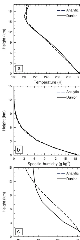
Table 1.Geophysical constants.
Parameter Value
Earth rotation rate =0 Coriolis parameter f=0
Mean Earth radius RE=6371.0 km Mean surface gravity g=9.79764 ms−2 Gas constant for dry air Rd=287.04 J kg−1K−1 Specific heat capacity for dry air Cpd=1004.64 J kg−1K−1 Water vapor gas constant Rv=461.50 J kg−1K−1 Water vapor specific heat capacity Cpv=1846.0 J kg−1K−1 Latent heat of vaporization at 0◦C Lv0=2.501×10⁶J kg−1 Latent heat of fusion at 0◦C Lf0=3.337×10⁵J kg−1 Latent heat of sublimation at 0◦C Ls0=2.834×10⁶J kg−1
model is initialized with the same temperature and moisture sounding at every grid point and zero wind, and convection is generated by prescribing some symmetry-breaking random noise. The model is then run to stationarity, at which time irradiances, precipitation, and other variables have stopped trending up or down and exhibit variability about an approx-imately constant value. Here, we consider RCE in a non-rotating setting; i.e., the Coriolis parameter, f, or Earth’s angular velocity,, is zero. Recommendations for geophys-ical constants and parameters are given in Table 1; models should use standard Earth values, following the convention of the Aqua-Planet Experiment (APE; http://climate.ncas.ac. uk/ape/design.html).
3.2.1 Surface boundary condition
The lower boundary condition is to be a spatially uniform, fixed sea surface temperature. If a skin temperature equation is employed, the skin temperature should be equal to the pre-scribed surface temperature. There is no sea ice and no land. The surface enthalpy fluxes are to be calculated interac-tively from the resolved surface wind speed and air–sea en-thalpy disequilibrium. Models should compute surface ex-change coefficients following their normal formulation, for instance, implying stability corrections, gustiness parameter-izations, or sea-state-dependent roughness formulations as is standard for their model tropics. If allowed by a model’s sur-face layer formulation, a minimum wind speed of 1 ms−1 should be enforced (either as V =max(Vresolved,1) or in quadrature asV =
q
Vresolved2 +1). We recognize that biases may result from the lack of boundary layer closure in some CRMs, but here we ask models to simply use their standard boundary layer scheme, if one exists.
3.2.2 Radiative processes
radia-Table 2.Radiation and initialization parameters.
Parameter Value
Radiation parameters
CO2concentration 348 ppmv CH4concentration 1650 ppbv N2O concentration 306 ppbv CFC11 concentration 0 CFC12 concentration 0 CFC22 concentration 0 CCL4 concentration 0
O3fit parameterg1 3.6478 ppmv hPa−g2 O3fit parameterg2 0.83209
O3fit parameterg3 11.3515 hPa Solar constant 551.58 W m−2
Zenith angle 42.05◦
Surface albedo 0.07
Analytic sounding parameters
zt 15 km
q0,295 12.00 g kg−1 q0,300 18.65 g kg−1 q0,305 24.00 g kg−1
qt 10−11g kg−1
zq1 4000 m
zq2 7500 m
0 0.0067 K m−1
p0 1014.8 hPa
tion scheme. GCMs that participate in CMIP6 (Eyring et al., 2016) should use the same radiation scheme as in CMIP6.
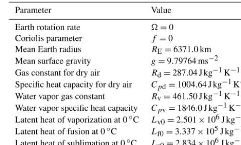
The climatologies of trace gases are to be adjusted so that they do not have any longitudinal and latitudinal dependen-cies, and their values should be fixed according to Table 2. The CO2concentration is to be set to 348 ppmv, CH4is to be 1650 ppbv, and N2O is to be 306 ppbv, following the conven-tion of the APE (http://climate.ncas.ac.uk/ape/design.html). Chlorofluorocarbon (CFC) concentrations are to be set to zero (following Popke et al., 2013). The ozone climatology is to be an analytic approximation of the horizontally uniform equatorial profile derived from the Aqua-Planet Experiment ozone climatology (Eq. 1, Fig. 1). The ozone volumetric mix-ing ratio, in units of parts per million, is to be computed from pressure using a gamma distribution:
O3=g1×pg2exp(−p/g3) , (1) where g1=3.6478, g2=0.83209, g3=11.3515, p is in hPa, and O3is in ppmv.
Aerosol effects are to be ignored by zeroing the aerosol concentrations. In some GCMs, aerosol effects may be ig-nored by excluding aerosol from the radiative transfer cal-culation and fixing the cloud droplet number concentration (we suggestNc=1.0×10⁸m−3) and ice crystal number con-centration (we suggest Ni=1.0×10⁵m−3) within the
mi-0 5 10
O3 concentration (ppmv)
0
50
100
150
200
Pressure (hPa)
(a)
0 5 10
O3 concentration (ppmv)
0
200
400
600
800
1000
Pressure (hPa)
(b)
Figure 1.Ozone concentration (ppm) from the Aqua-Planet Ex-periment (black) and gamma distribution given by Eq. (1) (green dashes), as a function of pressure above 200 hPa(a)and as a func-tion of pressure over the whole atmosphere(b).
crophysics parameterizations, following Reed et al. (2015). Cloud optical properties should be determined by the micro-physics parameterization. If specification of number concen-trations or condensation nuclei is required (as in two-moment schemes), GCMs should use the aqua-planet configuration of their microphysics. For those models that do not have an aqua-planet configuration (i.e., CRMs), if the microphysics scheme uses fixed cloud droplet and ice crystal number con-centration, we recommend these be set to the above values (Nc andNi). For those schemes that instead specify cloud condensation nuclei (CCN) and ice nuclei (IN), or CCN and IN sources, they should set values consistent with the above specifications ofNcandNi.
Importantly, the incoming solar radiation is to be adjusted such that every model grid point sees the same incident radia-tion. It is to be spatially uniform and constant in time; there is to be no diurnal cycle and no seasonal cycle. A reduced solar constant of 551.58 W m−2and a fixed zenith angle of 42.05◦ should be used (Table 2); these values yield an insolation of 409.6 W m−2, equal to the tropical (0–20◦) annual mean. The zenith angle is equal to the average insolation-weighted zenith angle between the Equator and 20◦(see Cronin, 2014).
3.2.3 Initialization procedure
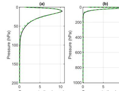
RCE_large, the large domain/global set of simula-tions, is to be initialized from the horizontally averaged equilibrium sounding of the corresponding RCE_small small-domain/single-column simulation. We request that RCE_small be initialized with the below analytic mois-ture (Eq. 2), temperamois-ture (Eq. 4) and pressure (Eq. 5) pro-file, and zero wind. The analytic sounding approximates the moist tropical sounding of Dunion (2011), enabling the use of an observed sounding while eliminating the need for inter-polation to different vertical grids. The parameter values for the analytic profile are found in Table 2. The analytic initial specific humidity profileq(z)is given, as a function of height (z) as
q(z)=q0exp
− z
zq1
exp "
−
z
zq2 2#
for 0≤z≤zt
q(z)=qtforz > zt, (2)
where zt=15 km approximates the tropopause height as seen in the Dunion (2011) sounding;q0is the specific humid-ity at the surface (z=0 km), which is taken to be 12 g kg−1 for the simulation at 295 K, 18.65 g kg−1 for the simulation at 300 K, and 24 g kg−1for the simulation at 305 K; andqtis the specific humidity in the upper atmosphere set to a con-stant value of 10−11g kg−1. The values ofq0have been ad-justed so that the relative humidity is near 80 % in the lower atmosphere for each SST value. The constant zq1 is set to 4000 m and the constant zq2 is set to 7500 m. The analytic initial virtual temperature profile is given by
Tv(z)=Tv0−0zfor 0≤z≤zt
Tv(z)=Tvtforz > zt, (3)
where the virtual temperature at the surface Tv0=
T0(1+0.608q0), the virtual temperature lapse rate 0 is 0.0067 K m−1, and the virtual temperature in the upper at-mosphere is the constantTvt=Tv0−0zt.T0is to be set to the SST value for each simulation (295, 300, or 305 K, re-spectively). The analytic initial temperature profile T (z)is thus
T (z)= Tv(z)
1+0.608q(z). (4)
The initial pressure profile p(z)is computed using the hy-drostatic equation and ideal gas law:
p(z)=p0 T
v0−0z Tv0
g/(Rd0)
for 0≤z≤zt
p(z)=ptexp
−
g(z−z t) RdTvt
forz > zt, (5)
where
pt=p0 Tvt
Tv0
g/(Rd0)
, (6)
and wherep0is the surface pressure 1014.8 hPa, andRdand gare given in Table 1. Code to compute this sounding from a specified set of height or pressure levels is provided on the RCEMIP website (http://myweb.fsu.edu/awing/rcemip. html). This analytic sounding shown in Fig. 2 is to be used only to begin the small-domain/single-column model simu-lations (RCE_small), not the large-domain/global simula-tions (RCE_large). It is worth nothing that this analytic setup is similar to that from Reed and Jablonowski (2011) used to initialize tropical environments in GCMs.
RCE_large, the large-domain/global simulations, should be initialized with average equilibrium profiles from the RCE_small simulations (at the corresponding SST). These equilibrium profiles should be derived by taking a horizontal and time mean of theRCE_smallsimulations, over the last 30 days of the 100-day simulation (i.e., after the simulation has reached statistical equilibrium). By starting from an equilibrium profile from the more computationally efficient RCE_small simulations, each RCE_large simulation will begin from that model’s own RCE state and thus eliminate the necessity of a lengthy spin-up period with large adjustments. Self-aggregation (which can be thought of as the instability of the RCE state; Emanuel et al., 2014) would be manifest as a large divergence away from the initial state. Care should be taken to ensure the settings of the RCE_smallsimulations match those of theRCE_large simulations.
For bothRCE_smallandRCE_large, symmetry is to be broken by prescribing a small amount of thermal noise in the five lowest layers (an amplitude of 0.1 K in the lowest layer, decreasing linearly to 0.02 K in the fifth layer). This will allow convection to start within the first few hours of each simulation.
We note that this procedure implies that stratospheric wa-ter vapor will be initialized with very small, but non-zero, specific humidities. It is unlikely that the stratospheric wa-ter vapor will be properly equilibrated by the end of the RCEMIP simulations, and so it is possible that this could af-fect the sensitivity of radiative fluxes to warming. The strato-spheric water vapor will thus need to be monitored and as-sessed in the evaluation of the simulations.
3.3 Model-type specific settings
single-Figure 2.Comparison of the analytic vertical profiles at 300 K to the observed Dunion (2011) moist tropical soundings of(a) temper-ature,(b)specific humidity, and(c)relative humidity (over liquid).
column models (SCMs), including those not tied to a parent GCM, is also possible. Below, we specify domain sizes and grid spacings for the required simulations but also encourage optional additional simulations with other grid spacings. In particular, we encourage large eddy simulations (LESs) with sub-kilometer grid spacings (see details in Sect. 3.3.2).
Table 3.CRM vertical grid for scalar variables.
Level Height Level Height Level Height
(m) (m) (m)
1 37 26 9000 51 21 500
2 112 27 9500 52 22 000
3 194 28 10 000 53 22 500
4 288 29 10 500 54 23 000
5 395 30 11 000 55 23 500
6 520 31 11 500 56 24 000
7 667 32 12 000 57 24 500
8 843 33 12 500 58 25 000
9 1062 34 13 000 59 25 500
10 1331 35 13 500 60 26 000
11 1664 36 14 000 61 26 500
12 2055 37 14 500 62 27 000
13 2505 38 15 000 63 27 500
14 3000 39 15 500 64 28 000
15 3500 40 16 000 65 28 500
16 4000 41 16 500 66 29 000
17 4500 42 17 000 67 29 500
18 5000 43 17 500 68 30 000
19 5500 44 18 000 69 30 500
20 6000 45 18 500 70 31 000
21 6500 46 19 000 71 31 500
22 7000 47 19 500 72 32 000
23 7500 48 20 000 73 32 500
24 8000 49 20 500 74 33 000
25 8500 50 21 000
3.3.1 CRMs
For all experiments, CRM simulations, that is, model simu-lations with explicit convection run on a limited-area planar domain, are to employ a three-dimensional domain with dou-bly periodic lateral boundary conditions. TheRCE_small simulations are to employ a square domain of ∼100 km length in each horizontal dimension and a horizontal grid spacing of∼1 km, which approximates the size of a GCM grid box.
TheRCE_largesimulations are to use a horizontal grid spacing of ∼3 km to resolve deep convection and cloud systems but reduce the computational cost. An elongated channel geometry of∼6000 km in the zonal direction and
The vertical grid will be stretched with at least 74 vertical levels with a model top no lower than 33 km and a sponge layer in the top model layers to damp gravity waves, follow-ing a given model’s usual prescription. Table 3 indicates the recommended vertical grid. The simulations should be run for at least 100 days.
3.3.2 GCMs
GCMs, that is, models with parameterized convection, should first be run in single-column mode forRCE_small, from which the equilibrium profile used to initialize the RCE_largeglobal simulations is derived.
For RCE_large, GCM simulations should employ a three-dimension spherical global domain using whichever dynamical core and grid are standard for each given model. Each model should use the horizontal resolution, vertical co-ordinate, and grid of one of their CMIP6 configurations. The simulations should be run for at least 3 years (∼1000 days). If the GCM has the capability to run in a planar configu-ration, it should also be run on the CRM grid described in Sect. 3.3.1 but with the GCM grid spacing and physics pa-rameterizations.
3.3.3 GCRMs
GCRMs, or models with explicit convection run on a non-rotating sphere, are an important category bridging CRMs and GCMs. Ideally, GCRMs should be run with the same grid spacing as CRMs and the same domain size as GCMs (that is, ∼3 km resolution and the real Earth radiusRE, respec-tively). Although recently more computer resources have be-come available for running GCRMs at such resolutions, we opt to define a more moderate specification of GCRM exper-iments such that more research groups running GCRMs are able to join RCEMIP. We propose two options: GCRM1, ar-bitrary horizontal resolution for the sphere with the Earth’s radius; and GCRM2,∼3 km horizontal grid spacing for an arbitrary radius of the sphere. Required integration time is the same as that of CRMs (100 days), and the other settings are also the same as those of CRMs or GCMs, as appropriate. In practice, relatively coarser resolutions than 3 km are used from GCRMs, though the resolution required to “re-solve” clouds explicitly is ambiguous. Resolutions of 7 and 14 km are frequently used for the Nonhydrostatic ICosahe-dral Atmospheric Model (NICAM), and even coarser resolu-tions have been used without convective parameterizaresolu-tions in NICAM (Yoshizaki et al., 2012; Takasuka et al., 2015) and other models (e.g., Webb et al., 2015; Becker et al., 2017). In addition, the definition of the horizontal resolution de-pends on grid structure and details of discretization which vary among GCRMs, so we recognize that it may not be pos-sible for all groups to use precisely the same resolution. If a smaller Earth radius is used, it can beRE/2,RE/4,RE/8, or RE/16 and so on (about 3200, 1600, 800, or 400 km,
respec-tively). The reduction of the Earth’s radius for global RCE studies has also been used in GCMs at hydrostatic scales (Reed and Medeiros, 2016).
The GCRM RCE_largesimulations should be initial-ized from a non-aggregated state, which can be obtained either from a simulation on a much smaller horizontal do-main (i.e., less than 200 km) or a simulation with horizontally homogenized radiative heating rates. We encourage GCRM groups to contact the RCEMIP organizers to discuss appro-priate model setups and coordinate with other groups. 3.3.4 SCMs
SCMs, or models with parameterized convection and a sin-gle grid column (no circulation), should be initialized using the analytic sounding described in Sect. 3.2.3 and should use whatever vertical grid is standard. If run in tandem with a par-ent GCM, care should be taken to ensure the settings and parameterizations are the same as in the global model. The simulations should be run for at least 3 years (∼1000 days). While SCM simulations are not able to address questions about convective aggregation itself, they may be compared to a parent GCM to determine the impact of convective ag-gregation on the RCE state (should agag-gregation occur in the global model). SCM simulations may also be compared to the otherRCE_smallsimulations (that is, to other SCMs and to non-aggregated small-domain CRM or LES simula-tions) to determine the robustness of the RCE state and the effectiveness of the SCM convective parameterization. 3.3.5 LES
LES, that is, models with explicit convection and sub-kilometer grid spacings that resolve the energy containing “large” turbulent eddies, may participate in RCEMIP by pro-viding a set of 50-day simulations on a small square domain of∼100 km length in each horizontal dimension with a hori-zontal grid spacing of∼50–100 m and∼100 vertical levels. The setup is similar to the CRM setup except any boundary layer parameterization should be turned off and any LES sub-grid model should be turned on. The LES model may be ini-tialized from the analytic sounding provided in Sect. 3.2.1, so that it can be compared to the correspondingRCE_smallat
∼1 km grid spacing. We encourage LES modelers to contact the RCEMIP organizers to discuss appropriate model setups and facilitate coordination with other groups.
4 Output specification
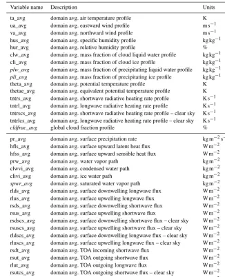
Table 4.The 1-D hourly-averaged variables (z, t) or (t). TOA indicates the top of atmosphere.
Variable name Description Units
ta_avg domain avg. air temperature profile K ua_avg domain avg. eastward wind profile m s−1 va_avg domain avg. northward wind profile m s−1 hus_avg domain avg. specific humidity profile kg kg−1 hur_avg domain avg. relative humidity profile % clw_avg domain avg. mass fraction of cloud liquid water profile kg kg−1 cli_avg domain avg. mass fraction of cloud ice profile kg kg−1
plw_avg domain avg. mass fraction of precipitating liquid water profile kg kg−1
pli_avg domain avg. mass fraction of precipitating ice profile kg kg−1 theta_avg domain avg. potential temperature profile K thetae_avg domain avg. equivalent potential temperature profile K tntrs_avg domain avg. shortwave radiative heating rate profile K s−1 tntrl_avg domain avg. longwave radiative heating rate profile K s−1 tntrscs_avg domain avg. shortwave radiative heating rate profile – clear sky K s−1 tntrlcs_avg domain avg. longwave radiative heating rate profile – clear sky K s−1
cldfrac_avg global cloud fraction profile % pr_avg domain avg. surface precipitation rate kg m−2s−1 hfls_avg domain avg. surface upward latent heat flux W m−2 hfss_avg domain avg. surface upward sensible heat flux W m−2 prw_avg domain avg. water vapor path kg m−2 clwvi_avg domain avg. condensed water path kg m−2 clivi_avg domain avg. ice water path kg m−2
spwr_avg domain avg. saturated water vapor path kg m−2 rlds_avg domain avg. surface downwelling longwave flux W m−2 rlus_avg domain avg. surface upwelling longwave flux W m−2 rsds_avg domain avg. surface downwelling shortwave flux W m−2 rsus_avg domain avg. surface upwelling shortwave flux W m−2 rsdscs_avg domain avg. surface downwelling shortwave flux – clear sky W m−2 rsuscs_avg domain avg. surface upwelling shortwave flux – clear sky W m−2 rldscs_avg domain avg. surface downwelling longwave flux – clear sky W m−2 rluscs_avg domain avg. surface upwelling longwave flux – clear sky W m−2 rsdt_avg domain avg. TOA incoming shortwave flux W m−2 rsut_avg domain avg. TOA outgoing shortwave flux W m−2 rlut_avg domain avg. TOA outgoing longwave flux W m−2 rsutcs_avg domain avg. TOA outgoing shortwave flux – clear sky W m−2 rlutcs_avg domain avg. TOA outgoing longwave flux – clear sky W m−2
For CRMs, the variables should be output on the model levels and on the nativex/ygrid. For GCMs, the variables should be output on model levels and the native grid (groups may addi-tionally interpolate to the standard CMIP6 pressure levels if they desire). If the native GCM grid is not latitude–longitude, then the output should also be interpolated to a latitude– longitude grid. The output format should be NetCDF, and will be uploaded to a shared data server, which will facilitate analysis and comparison of the simulations.
4.1 Variables
Table 4 indicates the list of one-dimensional statistics and domain-averaged profiles that are to be computed and output as hourly averages. The first half of the table includes vari-ables that are profiles (functions ofzandt), while the sec-ond half includes variables that are only a function of time. The italicized variables are non-standard outputs; all
oth-ers are standard CMIP6 output. The condensed water path, clwvi_avg, includes condensed (liquid plus ice) water, and includes precipitating hydrometeors only if the precipitating hydrometeors affect the calculation of radiative transfer in the model. The ice water path, clivi_avg, includes precipitat-ing frozen hydrometeors only if the precipitatprecipitat-ing hydrome-teors affect the calculation of radiative transfer in the model. The vertical coordinate and time coordinate should also be output. Relative humidity (hur_avg) should be computed with respect to liquid and ice, according to each model’s mi-crophysics scheme. We recommend that the Bolton formu-lation for equivalent potential temperature (thetae_avg) be used (Bolton, 1980, his Eq. 43).
Table 5.The 2-D hourly-averaged variables (x, y, t).
Variable name Description Units
pr surface precipitation rate kg m−2s−1 pr_conv! surface convective precipitation rate kg m−2s−1
evspsbl evaporation flux kg m−2s−1
hfls surface upward latent heat flux W m−2 hfss surface upward sensible heat flux W m−2 rlds surface downwelling longwave flux W m−2 rlus surface upwelling longwave flux W m−2 rsds surface downwelling shortwave flux W m−2 rsus surface upwelling shortwave flux W m−2 rsdscs surface downwelling shortwave flux – clear sky W m−2 rsuscs surface upwelling shortwave flux – clear sky W m−2 rldscs surface downwelling longwave flux – clear sky W m−2 rluscs surface upwelling longwave flux – clear sky W m−2 rsdt TOA incoming shortwave flux W m−2 rsut TOA outgoing shortwave flux W m−2 rlut TOA outgoing longwave flux W m−2 rsutcs TOA outgoing shortwave flux – clear sky W m−2 rlutcs TOA outgoing longwave flux – clear sky W m−2
prw water vapor path kg m−2
clwvi condensed water path kg m−2
clivi ice water path kg m−2
psl sea level pressure Pa
tas 2 m air temperature K
tabot* air temperature at lowest model level K
uas 10 m eastward wind m s−1
vas 10 m northward wind m s−1
uabot* eastward wind at lowest model level m s−1
vabot* northward wind at lowest model level m s−1
wa500ˆ vertical velocity at 500 hPa m s−1
wap500∼ omega at 500 hPa Pa s−1
spwr saturated water vapor path kg m−2 cl! total cloud fraction of grid column %
CRMs only. The variables with a (−)!symbol are outputs for GCMs only. Each model should output one or the other of the variables indicated with a symbol, depending on if they are in height (ˆ) or pressure-based (∼) coordinates. The horizontal coordinates and time coordinate should also be output.
Table 7 indicates the list of three-dimensional variables to output, as instantaneous 6-hourly snapshots. It is optional to upload these variables to the shared data server (we sug-gest uploading the last 25 days of 3-D output), but the 3-D variables must be saved and stored locally by each modeling group. The italicized variables are non-standard outputs; all others are standard CMIP6 output. The variables with a (−)! symbol are outputs for GCMs only. Note that each model should output omega or vertical velocity, and geopotential height or pressure, depending on whether the model is in pressure-based or height coordinates. Generally, CRMs are in height coordinates and GCMs are in a pressure-based co-ordinate such as hybrid sigma–pressure levels. Each model
should output one or the other of the variables indicated with a symbol, depending on if they are in height (ˆ) or pressure-based (∼) coordinates. The horizontal, vertical, and time co-ordinates should also be output.
4.2 Diagnostics 4.2.1 Cloud fraction
Table 6.The 2-D instantaneous hourly variables (x, y, t).
Variable name Description Units
fmse mass-weighted vertical integral of frozen moist static energy J m−2 hadvfmse mass-weighted vertical integral of horizontal advective tendency of frozen moist static energy J m−2s−1 vadvfmse mass-weighted vertical integral of vertical advective tendency of frozen moist static energy J m−2s−1 tnfmse total tendency of mass-weighted vertical integral of frozen moist static energy J m−2s−1 tnfmsevar total tendency of spatial variance of mass-weighted vertical integral of frozen moist static energy J2m−4s−1
Table 7.The 3-D instantaneous hourly variables (x, y, z, t).
Variable name Description Units
clw mass fraction of cloud liquid water g g−1
cli mass fraction of cloud ice g g−1
plw mass fraction of precipitating liquid water g g−1
pli mass fraction of precipitating ice g g−1
mc! convective mass flux kg m−2s−1
ta air temperature K
ua eastward wind m s−1
va northward wind m s−1
hus specific humidity g g−1
hur relative humidity %
wap∼ omega Pa s−1
waˆ vertical velocity m s−1
zg∼ geopotential height m
paˆ pressure Pa
tntr tendency of air temperature due to radiative heating K s−1 tntc! tendency of air temperature due to moist convection K s−1
tntrs tendency of air temperature due to shortwave radiative heating K s−1
tntrl tendency of air temperature due to longwave radiative heating K s−1
for all simulations. For GCMs, we also request the output of a total cloud fraction for each grid column as a 2-D variable (Table 5) under the variable name “cl”, which is a function ofx,y, andt.
4.2.2 Moist static energy budgets
We request that each modeling group estimate the moist static energy budget, as accurately as is possible. Specifically, we request the diagnosis and output of the additional 2-D instantaneous variables listed in Table 6. This (along with the other 2-D variables) will enable the quantification of the physical mechanisms related to self-aggregation (using the moist static energy variance budget as in Wing and Emanuel, 2014).
Frozen moist static energy is given by h=cpT+gz+ Lvq+Lfqice. The values ofcp,g,Lv, andLf used by the model formulation should be used to computeh.qice is the mass fraction of cloud ice. The mass-weighted vertical inte-gral of frozen moist static energy (fmse) is given by
bh= ztop
Z
0
cpT+gz+Lvq+Lfqiceρdz, (7)
or, in pressure coordinates,
eh= 1 g
psfc
Z
ptop
cpT+gz+Lfqicedp. (8)
Care should be taken to make sure the same limits of inte-gration are used at all times/locations. The mass-weighted vertical integral of horizontal advective tendency of frozen moist static energy (hadvfmse) is given by
ztop
Z
0
u∂h ∂x+v
∂h ∂y
and the mass-weighted vertical integral of the vertical ad-vective tendency of frozen moist static energy (vadvfmse) is given by
ztop
Z
0 w∂h
∂zρdz. (10)
Ideally, frozen moist static energy would be diagnosed on-line and each model’s advection scheme used to advect it, but if this is not possible we ask that groups make their best effort to estimate these terms. The spatial variance of the mass-weighted vertical integral of frozen moist static energy is computed using the squared anomalies from the horizontal mean of the mass-weighted vertical integral of moist static energy (bh). Its tendency (tnfmsevar) is given by
∂ ∂t
ztop
Z
0 hρdz
02
, (11)
where0indicates an anomaly from the horizontal mean. 4.2.3 Aggregation metrics
We expect that the phenomenon of self-aggregation may oc-cur in some simulations and therefore request the diagno-sis of the following metrics that may be used to character-ize the degree of aggregation. Code for these (and other) diagnostics will be provided on the RCEMIP website (http: //myweb.fsu.edu/awing/rcemip.html).
1. The “organization index” (Iorg) was introduced by Tompkins and Semie (2017) as an index of aggregation in CRM simulations based on the distribution of near-est neighbor distance between convective entities. If the system exhibits random convection behaving as a Pois-son point process,Iorgwould be equal to 0.5. Therefore, values ofIorggreater than 0.5 indicate aggregated con-vection, with higher values indicating a higher degree of organization. Tompkins and Semie (2017) used a verti-cal velocity threshold of 1 ms−1at 730 hPa to define up-draft grid cells in CRM simulations of self-aggregation. Cronin and Wing (2017) compared using a vertical ve-locity threshold and a cloud top temperature thresh-old to defineIorgin simulations of self-aggregation and found that, while the absolute values of Iorg differed, their tendencies were the same. Therefore, given that RCEMIP includes both CRM and GCM simulations and that a vertical velocity threshold may not be appropri-ate for GCM simulations, here we suggest defining con-vective grid cells as grid boxes with values of outgoing longwave radiation less than 173 W m−2.
2. The “subsidence fraction” (SF) uses the fractional area of the domain covered by large-scale subsidence in the
Upward LW radiation at TOA
100 W m-2 320 W m-2
P (mm h )
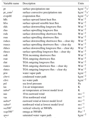
0.648 1.33 2.73 5.62 11.5 23.7 48.6 99.9 205 421 865 OLR and precipitation, day 90.7083
0 20 40 60 80
x (km) 0
10 20 30 40 50 60 70 80 90
y (km)
-1
Figure 3.Hourly-average OLR (gray shading) and precipitation (color shading) in small-domain System for Atmospheric Model-ing (SAM) simulation atTs=300 K.
mid-troposphere (w <0 or ω >0 at 500 hPa) to char-acterize the degree of aggregation (Coppin and Bony, 2015). SF is less than 0.6 when convection is unor-ganized and greater than 0.6 when it is aggregated. For CRM simulations, the vertical velocity at 500 hPa should be averaged over 1 day and over a suitably large area (∼100 km, to approximate the size of a GCM grid cell).
5 Sample results
Table 8 shows a preliminary list of models that are con-firmed to participate in RCEMIP. We expect this list to grow with participation from other modeling groups and scientists across the world.
Table 8.Preliminary list of participating models.
Model Acronym Model Type Citation
Community Atmosphere Model, version 5 CAM5 GCM Neale et al. (2012)
Community Atmosphere Model, version 6 CAM6 GCM TBD
ECHAM6 ECHAM6 GCM Popke et al. (2013)
ICOsahedral Nonhydrostatic Model ICON CRM/GCRM/GCM Dipankar et al. (2015)
IPSL-CM5A-LR IPSL-CM5A-LR GCM Dufresne et al. (2013)
IPSL-CM6 IPSL-CM6 GCM TBD
Nonhydrostatic ICosahedral Atmospheric Model,
version 15 NICAM.15 GCRM Satoh et al. (2014)
System for Atmospheric Modeling SAM CRM Khairoutdinov and Randall (2003) UCLA Large-Eddy Simulation Model UCLA-LES CRM Hohenegger and Stevens (2016)
Upward LW radiation at TOA 100 W m-2 320 W m-2
P (mm h )
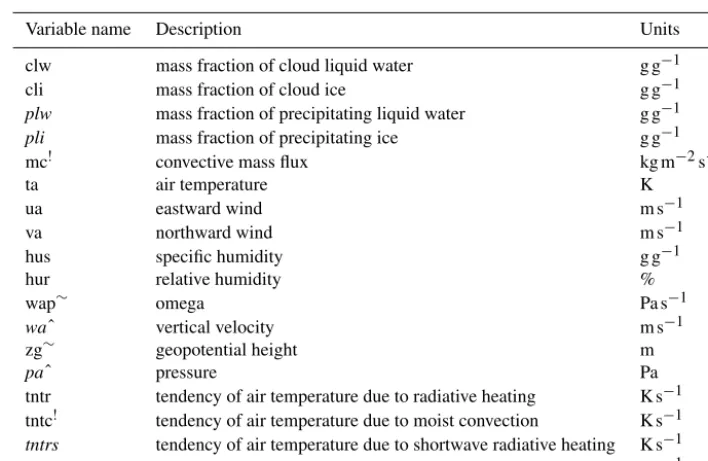
0.648 1.33 2.73 5.62 11.5 23.7 48.6 99.9 205 421 865 OLR and precipitation, day 90.7083
0 1000 2000 3000 4000 5000 6000
x (km)
0 100 200 300
y (km)
-1
Figure 4.Hourly-average outgoing longwave radiation (gray shading) and precipitation (color shading) in large-domain SAM simulation at
Ts=300 K.
(a) Day 10 water vapor path (kg m-2)
0 1000 2000 3000 4000 5000 6000
x (km) 0
100 200 300
y (km) 20
40 60
(b) Day 90 water vapor path (kg m-2)
0 1000 2000 3000 4000 5000 6000
x (km) 0
100 200 300
y (km) 20
40 60
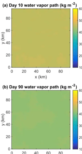
Figure 5.Daily mean water vapor path (computed from hourly averages) on day 10(a)and day 90(b)of the large-domain SAM simulation atTs=300 K.
Figures 3–7 show example results from a cloud-resolving model simulation of RCE, using SAM with the settings configured as described in Sect. 3.3.1 (with the exception of the q0 values in the analytic profiles used to initial-ize the RCE_small simulations at 295 and 305 K; q0= 18.65 g kg−1was used for all simulations shown here). Fig-ure 3 shows outgoing longwave radiation (indicating deep convective clouds) and precipitation rate from the end of aRCE_smallsimulation at 300 K; the convection is quasi-random in space and time. Figure 4 shows outgoing long-wave radiation and precipitation rate from a RCE_large simulation at 300 K. The convection is aggregated into sev-eral large clusters. Self-aggregation is characterized by the
feed-(a) Day 10 water vapor path (kg m-2)
0 20 40 60 80 x (km) 0
20 40 60 80
y (km)
10 20 30 40 50 60
(b) Day 90 water vapor path (kg m-2)
0 20 40 60 80 x (km) 0
20 40 60 80
y (km)
10 20 30 40 50 60
Figure 6.Daily mean water vapor path (computed from hourly av-erages) on day 10 (a)and day 90(b) of the small-domain SAM simulation atTs=300 K.
backs to that growth in moist static energy variance; in this case, it is the surface flux and longwave radiation feedbacks. Figure 8 shows an example result from a global simulation of RCE with explicit convection, using NICAM in a global, non-rotating, spherical configuration with a real Earth radius and a 14 km horizontal grid spacing. Figure 8 shows a snap-shot of outgoing longwave radiation (OLR) and precipita-tion rate, which is similar to Figs. 3–4. The convecprecipita-tion has spontaneously organized into clusters. Differences in aggre-gation properties, such as cluster sizes, can be seen between the results shown in Figs. 4 and 8, which may stem from the domain geometry, the horizontal resolution, or other de-tails, as mentioned in Sect. 3.3.1. Note that, in this exam-ple simulation, slightly different values of the solar constant, zenith angle, surface albedo, and minimum wind speed in the surface flux calculation were used than those described in the RCEMIP protocol (434 W m−2, 0◦, and 2 ms−1, respec-tively). The simulation was initialized from zonally averaged profiles of a coarser-resolution simulation.
Figures 9–10 show example results from a series of GCM simulations of RCE, using CAM5 with the spectral element dynamical core on a cubed–sphere grid with ne30 resolution, which corresponds to ∼100 km grid spacing. More details on the version of CAM5 (including the physics packages)
0 20 40 60 80 100
1012 1013 1014 1015
(J/m
2)
2
20 40 60 80
Time (days)
-2 -1 0 1 2
days
-1
Longwave Shortwave Surface flux Advective
Figure 7.Domain average frozen moist static energy (FMSE) vari-ance(a)and terms in domain average FMSE variance budget, nor-malized by domain average FMSE variance(b) from the large-domain SAM simulation atTs=300 K.
used for these simulations can be found in Reed et al. (2015). Figure 9 shows a snapshot of OLR and precipitation rate for the set of three RCEMIP experiments, which can be com-pared to Figs. 3, 4, and 8. Figure 10 shows a snapshot of water vapor path (at the same time as displayed in Fig. 9). There is a large cluster of clouds and precipitation in each of the simulations at 300 and 305 K, while the precipitation in the simulation at 295 K is somewhat more scattered. The simulation at 305 K appears to be the most aggregated, with a single hemisphere-scale, intensely precipitating cluster and little cloud cover or precipitation elsewhere on the globe. It is also evident from Fig. 10 that the range of water vapor path values is largest in the simulation at 305 K, with the largest values occurring where the clouds and precipitation are clus-tered.
0.648 1.33 2.73 5.62 11.5 23.7 48.6 99.9 205 421 865 Upward longwave radiation at TOA [W m ]-2
Precipitation rate [mm h ]
100 120 140 160 180 200 220 240 260 280 300 320
-1
Figure 8.Hourly-averaged OLR at the top of atmosphere (gray shading) and precipitation rate (color shading) in a NICAM simulation at
Ts=300 K. Note that several parameters do not precisely follow the RCEMIP protocol.
aggregation). The degree of convective aggregation can be diagnosed using the subsidence fraction metric, for example (SF; Sect. 4.2.3). In the SAM CRM simulation, the subsi-dence fraction increases over the first∼40 days of each sim-ulation, indicating the increasing aggregation of convection and development of large areas of subsiding air (Fig. 12). The mean subsidence fraction over the last 25 days decreases with increasing SST, but there is large variability in the subsidence fraction. The equilibrium value of the subsidence fraction is between∼0.65 and 0.7 in the SAM simulations, while it is higher (∼0.7–0.8) in the NICAM and CAM simulations, in-dicating that the convection is more aggregated in the global simulations. The subsidence fraction does not depend mono-tonically on SST in either the NICAM or CAM simulations.
6 Extensions of RCEMIP
RCEMIP has been designed to be as simple as possible in order to maximize participation, foster a community of mod-elers of RCE, and allow for scientific progress on each of our three themes with a minimum of simulations. We recognize that the initial simulations will not necessarily be a defini-tive representation of the RCE state, for reasons such as lack of boundary closure in some CRMs, distortions of shallow clouds, sensitivity to microphysical formulations, and other sources of bias that we might not be aware of yet. Our vi-sion for the evolution of RCEMIP is that the simulations proposed here serve as a starting point that will allow us to establish a baseline, enable progress on the scientific ob-jectives presented in Sect. 2, and based on the results,
in-form subsequent experimentation. RCEMIP presents an ex-ceptional opportunity for the participants to explore other is-sues, which we hope will form the basis for a second phase of RCEMIP. Here, we provide a few suggestions that we think are promising avenues forward but leave open the possibility for other directions that could evolve from the results of the first RCEMIP simulations.
6.1 Robustness of RCE results to experimental design Additional simulations could be performed to assess the sen-sitivity of the results to the model setup/configuration (for example, the impact of the lower boundary conditions, de-pendence on domain size and resolution, and dede-pendence on the initial conditions of convective organization).
promis-1 (a)
(b)
(c)
Figure 9.Hourly-averaged snapshot of upward longwave radiation at the top of atmosphere (OLR; gray shading) and precipitation rate (color shading) from the last day (day 1095) of the three CAM sim-ulations atTs=295 K(a),Ts=300 K(b), andTs=305 K(c).
ing avenue forward to determine the sensitivity of the RCE state to model setup, dynamics, and physics is to design uni-fied and simple representations of parameterized processes, as, for instance, was used to study stratocumulus clouds in the GEWEX Cloud System Study (GCSS) intercomparison (Bretherton et al., 1999). Such a setup would reduce the ever-increasing complexity of parameterizations and thus may be useful for identifying the origin of differences between mod-els. In particular, we expect large differences to occur based on the diversity in the treatment of microphysics, and be-cause of the neglect of the boundary layer in some CRMs. Jeevanjee et al. (2017), in arguing for an “elegant” RCE con-figuration, suggested that the adoption of a simple, warm-rain, Kessler-type microphysics scheme would ease compar-ison between models with regards to cloud fraction and cloud radiative effects, for example. Simplified treatments of cloud
(a)
(b)
(c)
Figure 10. Hourly-averaged water vapor path from the last day (day 1095) of the three CAM simulations atTs=295 K(a),Ts= 300 K(b), andTs=305 K(c).
optical properties for radiative transfer and boundary layer closures could also be designed, as could a simple micro-physics scheme that includes frozen precipitation.
6.3 Mechanisms of convective aggregation
More in-depth investigation into how the mechanisms of con-vective aggregation vary across models, including their spa-tial scale and hysteresis, would be valuable. The inispa-tial sim-ulations of RCEMIP (Sect. 3) are a good starting point for studying self-aggregation, but further experiments could be defined to leverage the opportunity afforded by RCEMIP to make progress on some of the unanswered questions laid out by Wing et al. (2017). These questions include the behav-ior of self-aggregation when subjected to mean winds and/or vertical wind shear, simulated over a land surface, or simu-lated over an ocean mixed layer with interactive SST. 6.4 Impact of ocean–atmosphere interactions
0 0.1 0.2 0.3
Cloud fraction
200
400
600
800
1000
Pressure, hPa
(a) SAM-Small Domain
295 K 300 K 305 K
0 0.1 0.2 0.3
Cloud fraction
200
400
600
800
1000
Pressure, hPa
(b) SAM-Large Domain
0 0.1 0.2 0.3
Cloud fraction
200
400
600
800
1000
Pressure, hPa
(c) NICAM
0 0.1 0.2 0.3
Cloud fraction
200
400
600
800
1000
Pressure, hPa
(d) CAM
Figure 11.Profiles of total global cloud fraction from the (a)small-domain SAM simulations,(b) large-domain SAM simulations,(c)
NICAM simulations, and(d) CAM simulations. The SAM data are averaged over the last 25 days of simulation, the NICAM data are averaged over the last 20 days of simulation, and the CAM data are averaged over the last 2 years of simulation. Note that the NICAM simulations do not precisely follow the RCEMIP protocol, and the NICAM simulations labeled 295 and 305 K are actually performed at surface temperatures of 296 and 304 K, respectively.
Time (days)
0 50 100
SF
0.5 0.55 0.6 0.65 0.7 0.75 0.8
0.85 (a) SAM
295 K 300 K 305 K
Time (days)
0 50 100 150 200
SF
0.5 0.55 0.6 0.65 0.7 0.75 0.8
0.85 (b) NICAM
Time (days)
0 200 400 600 800 1000 1200
SF
0.5 0.55 0.6 0.65 0.7 0.75 0.8
0.85 (c) CAM
Figure 12.Subsidence fraction (SF) as a function of time in the(a)large-domain SAM simulations,(b)NICAM simulations and(c)CAM simulations. The circles indicate the mean subsidence fraction over the last 25 days of simulation; the error bars indicate the bounds of the 5–95 % confidence interval. Note that the time axes are different in each panel. Also note that the NICAM simulations do not precisely follow the RCEMIP protocol, and the NICAM simulations labeled 295 and 305 K are actually performed at surface temperatures of 296 and 304 K, respectively.
to an ocean mixed layer, it would be possible to study the in-fluence of air–sea coupling on the interplay between surface temperature and convective aggregation, which has found to be critical in some models (e.g., Coppin and Bony, 2015). An abrupt 4×CO2experiment run with such a model would also help assess the RCE response to CO2forcing, including the adjustment of tropospheric clouds, and the climate sensi-tivity.
6.5 Impact of rotation
RCEMIP has been designed to simulate RCE in a non-rotating framework, but there is a growing body of work simulating rotating RCE, in which convective aggregation takes the form of spontaneous genesis of tropical cyclones (e.g., Held and Zhao, 2008; Khairoutdinov and Emanuel, 2013; Zhou et al., 2014; Shi and Bretherton, 2014; Reed and Chavas, 2015; Wing et al., 2016). Such simulations can be
performed on a limited-area domain with uniform rotation, a global domain with uniform rotation, or a global domain with spherically varying rotation.
7 Conclusions
sensitivity, and the aggregation of convection and its role in climate. In addition, the simple premise of RCE will allow the results of RCEMIP to be connected to theory, as well as serve as a useful framework for model development and evaluation. RCEMIP distinguishes itself from many other in-tercomparisons because of its ability to involve many model types (SCMs, CRMs, GCRMs, GCMs, LES); the comparison between model types is vital as increasingly higher resolu-tions are possible in climate-scale global modeling. RCEMIP is specifically designed to determine how models of differ-ent types represdiffer-ent the same phenomena and thus provides a basis for testing models with parameterized convection against models that simulate convection directly. In doing so, RCEMIP will help us answer some of the most important questions in climate science.
Code and data availability. Scripts to calculate the analytic sound-ing described in Sect. 3.2.3 and the diagnostics described in Sect. 4.2 will be available on the RCEMIP website at http://myweb. fsu.edu/awing/rcemip.html. The model output from RCEMIP will be made publicly available through the WDCC/CERA archive at DKRZ, accessible at https://cera-www.dkrz.de/WDCC/ ui/cerasearch/.
Author contributions. AAW led the writing of the text. All authors contributed to editing the text and discussing the goals and specifi-cations of RCEMIP.
Competing interests. The authors declare that they have no conflict of interest.
Acknowledgements. RCEMIP arose from discussion at the Model Hierarchies Workshop, sponsored by the Working Group on Climate Modeling of the World Climate Research Programme and held in Princeton, NJ, in November 2016. The authors thank Nadir Jeevanjee, Timothy Cronin, Kerry Emanuel, George Bryan, and Travis O’Brien for helpful feedback and discussion, as well as Isaac Held, Levi Silvers, and two anonymous reviewers for constructive reviews that improved the design and presentation of RCEMIP. The SAM cloud-resolving model, from which results were shown in Sect. 5, is maintained and provided by Marat Khairoutdinov.
Edited by: Chiel van Heerwaarden
Reviewed by: Levi Silvers, Isaac Held, and two anonymous referees
References
Arnold, N. P. and Randall, D. A.: Global-scale convec-tive aggregation: implications for the Madden-Julian Oscillation, J. Adv. Model. Earth Syst., 7, 1499–1518, https://doi.org/10.1002/2015MS000498, 2015.
Becker, T. and Stevens, B.: Climate and climate sensitivity to chang-ing CO2on an idealized land planet, J. Adv. Model. Earth Syst., 6, 1205–1223, https://doi.org/10.1002/2014MS000369, 2014. Becker, T., Hohenegger, C., and Stevens, B.: Imprint of the
convec-tive parameterization and sea-surface temperature on large-scale convective self-aggregation, J. Adv. Model. Earth Syst., 9, 1488– 1505, https://doi.org/10.1002/2016MS000865, 2017.
Bolton, D.: The Computation of equivalent potential temperature, Mon. Weather Rev., 108, 1046–1053, 1980.
Bony, S., Stevens, B., Frierson, D. M. W., Jakob, C., Kageyam, M., Pincus, R., Shepherd, T. G., Sherwood, S. C., Siebesma, A. P., Sobel, A. H., Watanabe, M., and Webb, M. J.: Clouds, cir-culation and climate sensitivity, Nat. Geosci., 8, 261–268, https://doi.org/10.1038/ngeo2398, 2015.
Bony, S., Stevens, B., Coppin, D., Becker, T., Reed, K. A., Voigt, A., and Medeiros, B.: Thermodynamic control of anvil cloud amount, P. Natl. Acad. Sci. USA, 113, 8927–8932, https://doi.org/10.1073/pnas.1601472113, 2016.
Boucher, O., Randall, D., Artaxo, P., Bretherton, C., Feingold, G., Forster, P., Kerminen, V.-M., Kondo, Y., Liao, H., Lohmann, U., Rasch, P., Satheesh, S., Sherwood, S., Stevens, B., and Zhang, X.: Clouds and aerosols, in: Climate Change 2013: The Physical Sci-ence Basis, IPCC, Cambridge Univ. Pres, Cambridge, 571–657, 2013.
Bretherton, C. S., Macvean, M., Bechtold, P., Chlond, A., Cot-ton, W. R., Cuxart, J., Cuijpers, H., Khairoutdinov, M., Koso-vic, B., Lewellen, D., Moeng, C.-H., Siebesma, P., Stevens, B., Stevens, D., Sykes, I., and Wyant, M.: An intercomparison of radiatively-driven entrainment and turbulence in a smoke cloud, as simulated by different numerical models, Q. J. Roy. Meteor. Soc., 125, 391–423, 1999.
Bretherton, C. S., Blossey, P. N., and Khairoutdinov, M.: An energy-balance analysis of deep convective self-aggregation above uniform SST, J. Atmos. Sci., 62, 4237–4292, https://doi.org/10.1175/JAS3614.1, 2005.
Byrne, M. P. and Schneider, T.: Narrowing of the ITCZ in a warming climate: physical mechanisms, Geophys. Res. Lett., 43, 11350–11357, https://doi.org/10.1002/2016GL070396, 2016. Byrne, M. P. and Schneider, T.: Atmospheric dynamics
feed-back: concept, simulations and climate implications, J. Climate, https://doi.org/10.1175/JCLI-D-17-0470.1, in press, 2018. Charney, J. G., Arakawa, A., Baker, D. J., and Bolin, B.: Carbon
Dioxide and Climate: A Scientific Assessment, National Re-search Council, Woods Hole, MA, 1979.
Chavas, D. R. and Emanuel, K. A.: Equilibrium tropical cyclone size in an idealied state of radiative-convective equilibrium, J. Atmos. Sci., 71, 1663–1680, https://doi.org/10.1175/JAS-D-13-0155.1, 2014.
spectrum of climate system models, Clim. Dynam., 18, 579–586, 2002.
Coppin, D. and Bony, S.: Physical mechanisms controlling the initiation of convective self-aggregation in a General Cir-culation Model, J. Adv. Model. Earth Syst., 7, 2060–2078, https://doi.org/10.1002/2015MS000571, 2015.
Cronin, T. W.: On the choice of average solar zenith angle, J. Atmos. Sci., 71, 2994–3003, https://doi.org/10.1175/JAS-D-13-0392.1, 2014.
Cronin, T. W. and Wing, A. A.: Clouds, circulation, and cli-mate sensitivity in a radiative-convective equilibrium chan-nel model, J. Adv. Model. Earth Syst., 9, 2833–2905, https://doi.org/10.1002/2017MS001111, 2017.
Cronin, T. W., Emanuel, K., and Molnar, P.: Island precipita-tion enhancement and the diurnal cycle in radiative-convective equilibrium, Q. J. Roy. Meteorol. Soc., 141, 1017–1034, https://doi.org/10.1002/qj.2443, 2015.
Dines, W. H.: The heat balance of the atmosphere, Q. J. Roy. Mete-orol. Soc., 43, 151–158, 1917.
Dipankar, A., Stevens, B., Heinze, R., Moseley, C., Zängl, G., Gior-getta, M., and Brdar, S.: Large eddy simulation using the general circulation model ICON, J. Adv. Model. Earth Syst., 7, 963–986, https://doi.org/10.1002/2015MS000431, 2015.
Dufresne, J.-L., Foujols, M.-A., Denvil, S., Caubel, A., Marti, O., Aumont, O., Balkanski, Y., Bekki, S., Bellenger, H., Ben-shila, R., Bony, S., Bopp, L., Braconnot, P., Brockmann, P., Cadule, P., Cheruy, F., Codron, F., Cozic, A., Cugnet, D., de Noblet, N., Duvel, J.-P., Ethé, C., Fairhead, L., Fichefet, T., Flavoni, S., Friedlingstein, P., Grandpeix, J.-Y., Guez, L., Guil-yardi, E., Hauglustaine, D., Hourdin, F., Idelkadi, A., Ghat-tas, J., Joussaume, S., Kageyama, M., Krinner, G., Labetoulle, S., Lahellec, A., Lefebvre, M.-P., Lefevre, F., Levy, C., Li, Z., Lloyd, J., Lott, F., Madec, G., Mancip, M., Marchand, M., Masson, S., Meurdesoif, Y., Mignot, J., Musat, I., Parouty, S., Polcher, J., Rio, C., Schulz, M., Swingedouw, D., Szopa, S., Talandier, C., Terray, P., Viovy, N., and Vuichard, N.: Cli-mate change projections using the IPSL-CM5 Earth System Model: from CMIP3 to CMIP5, Clim. Dynam., 40, 2123–2165, https://doi.org/10.1007/s00382-012-1636-1, 2013.
Dunion, J.: Rewriting the climatology of the Tropical North At-lantic and Caribbean Sea atmosphere, J. Climate, 24, 893–908, https://doi.org/10.1175/2010JCLI3496.1, 2011.
Emanuel, K., Wing, A. A., and Vincent, E. M.: Radiative-convective instability, J. Adv. Model. Earth Syst., 6, 75–90, https://doi.org/10.1002/2013MS000270, 2014.
Eyring, V., Bony, S., Meehl, G. A., Senior, C. A., Stevens, B., Stouffer, R. J., and Taylor, K. E.: Overview of the Coupled Model Intercomparison Project Phase 6 (CMIP6) experimen-tal design and organization, Geosci. Model Dev., 9, 1937–1958, https://doi.org/10.5194/gmd-9-1937-2016, 2016.
Grabowski, W., Moncrieff, M., and Kiehl, J.: Long-term behavior of precipitating tropical cloud systems: a numerical study, Q. J. Roy. Meteorol. Soc., 122, 1019–1042, 1996.
Held, I. M. and Zhao, M.: Horizontally homogeneous rotating radiative-covnective equilibrium at GCM resolution, J. Atmos. Sci., 65, 2003–2013, https://doi.org/10.1175/2007JAS2604.1, 2008.
Held, I. M., Hemler, R. S., and Ramaswamy, V.: Radiative-convective equilibrium with explicity two-dimensional moist convection, J. Atmos. Sci., 50, 3909–3927, 1993.
Held, I. M., Zhao, M., and Wyman, B.: Dynamic radiative-convective equilibria using GCM column physics, J. Atmos. Sci., 64, 228–238, https://doi.org/10.1175/JAS3825.11, 2007. Hohenegger, C. and Stevens, B.: Coupled radiative
convec-tive equilibrium simulationswith explicit and parameterized convection, J. Adv. Model. Earth Syst., 8, 1468–1482, https://doi.org/10.1002/2016MS000666, 2016.
Holloway, C. E., Wing, A. A., Bony, S., Muller, C., Masunaga, H., L’Ecuyer, T. S., Turner, D. D., and Zuidema, P.: Observing con-vective aggregation, Surv. Geophys., 38, 1199–1236, 2017. Ingram, W.: A very simple model for the water vapour
feed-back on climate change, Q. J. Roy. Meteorol. Soc., 136, 30–40, https://doi.org/10.1002/qj.546, 2010.
Islam, S., Bras, R. L., and Emanuel, K. A.: Predictability of mesoscale rainfall in the tropics, J. Appl. Meteorol., 32, 297– 310, 1993.
Jeevanjee, N. and Romps, D. M.: Invariant radiative cooling and mean precipitation change, Atmospheric and Oceanic Physics, available at: https://arxiv.org/abs/1711.03516v1, last access: 15 December 2017.
Jeevanjee, N., Hassanzadeh, P., Hill, S. A., and Sheshadri, A.: A perspective on climate model hierarchies, J. Adv. Model. Earth Syst., 9, 1760–1771, https://doi.org/10.1002/2017MS001038, 2017.
Khairoutdinov, M. and Randall, D.: Cloud resolving modeling of the ARM Summer 1997 IOP: model formulation, results, uncer-tainties, and sensitivities, J. Atmos. Sci., 60, 607–625, 2003. Khairoutdinov, M. F. and Emanuel, K. A.: Aggregation of
con-vection and the regulation of tropical climate, Preprints, in: 29th Conference on Hurricanes and Tropical Meteorology, Amer. Meteorol. Soc., Tucson, AZ, 2010.
Khairoutdinov, M. F. and Emanuel, K.: Rotating radiative-convective equilibrium simulated by a cloud-resolving omdel, J. Adv. Model. Earth Syst., 5, 816–825, https://doi.org/10.1002/2013MS000253, 2013.
Manabe, S. and Strickler, R. F.: Thermal equilibriation of the atmo-sphere with a convective adjustment, J. Atmos. Sci., 21, 361–385, 1964.
Manabe, S. and Wetherald, R. T.: Thermal equilibrium of the atmo-sphere with a given distribution of relative humidity, J. Atmos. Sci., 24, 241–259, 1967.
Mauritsen, T. and Stevens, B.: Missing iris effect as a possible cause of muted hydrological change and high climate sensitivity in models, Nat. Geosci., 8, 346–351, https://doi.org/10.1038/ngeo2414, 2015.
Möller, F.: On influence of changes in CO2concentration in air on radiation balance of earths surface and on climate, J. Geophys. Res., 68, 3877–3886, 1963.
Muller, C. J.: Impact of convective organization on the response of tropical precipitation extremes to warming, J. Climate, 26, 5028– 5043, https://doi.org/10.1174/JCLI-D-12-00655.1, 2013. Muller, C. J. and Held, I. M.: Detailed investigation of the