DEPARTMENT OF CIVIL, ENVIRONMENTAL AND MECHANICAL ENGINEERING
Doctoral School in Department of Civil, Environmental and Mechanical Engineering
XXIX cycle
Numerical Methods for Compressible Multi-phase
flows with Surface Tension
Nguyen Tri Nguyen
Advisor
Prof. Michael Dumbser
Universit`
a degli Studi di Trento
Abstract
In this thesis we present a new and accurate series of computation methods for com-pressible multi-phase flows with capillary effects based upon the full seven-equation Baer-Nunziato model. For that reason, there are some numerical methods to obtain high accuracy solutions, which will be shown here. First, a high resolution shock capturing Total Variation Diminishing (TVD) finite volume scheme is used on both Cartesian and unstructured triangular grids. Regarding the TVD finite volume scheme on the unstruc-tured grid, time-accurate local time stepping (LTS) is applied to compute the solutions of the governing PDE system, in which the results are also compared with time-accurate global time stepping. Second, we propose a novel high order accurate numerical method for the solution of the seven equation Baer-Nunziato model based on ADER discontinuous Galerkin (DG) finite element schemes combined with a posteriori subcell finite volume limiting and adaptive mesh refinement (AMR).
In multi-phase flows, the difficulty is to design accurate numerical methods for resolving the phase interface, as well as the simulation of the phenomena occurring at the interface, such as surface tension effects, heat transfer and friction. This is because of the inter-actions of the fluids at the phase interface and its complex geometry. So the accurate simulation of compressible multi-phase flows with surface tension effects is currently still one of the most challenging problems in computational fluid dynamics (CFD). In this work, we present a novel path-conservative finite volume discretization of the continuum surface force method (CSF) of Brackbill et al. to account for the surface tension effect due to curvature of the phase interface. This is achieved in the context of a diffuse interface approach, based on the seven equation BaerNunziato model of compressible multi-phase flows. Such diffuse interface methods for compressible multi-phase flows including capil-lary effects have first been proposed by Perigaud and Saurel. Regarding the high order accuracy of a diffuse interface approach, the interface is captured and allowed to travel across one single possibly refined cell, and is computed in the context of multi-dimensional
high accurate space/time DG schemes with AMR and a posteriori sub-cell stabilization. The surface tension terms of the CSF approach are considered as a part of the non-conservative hyperbolic system. We propose to integrate the CSF source term as a non-conservative product and not simply as a source term, following the ideas on path-conservative finite volume schemes put forward by Castro and Par´es.
the memory of my grandmother Pham Thi Cat (1936 - 2014).
Acknowledgements
My sincere appreciation and deep respect to my supervisor, Professor Michael Dumbser, for his unlimited support with continuous and patient advice during my studies. Much of this work could not have been achieved without his ideas, encouragement, thorough review, and dedication.
I would like to thank all the members of the numerical analysis group for helping me one way or another during my studies at DICAM, Trento University, Italy. I also would like to thank Trento University for providing the funding for supporting my research.
Last but not least, I would like to express my loving thanks to my wife Vu Thi Kim Yen, my daughter Nguyen Vu Thien Minh, and my parents. They always helped me in sharing my difficulties throughout the years of my studies.
Contents
List of Tables ix
List of Figures xii
Symbols xvii
Abbreviations xix
1. Introduction 1
1.1. Introduction . . . 1
1.2. The compressible Euler and Navier-Stokes equations for single phase flows 6 1.2.1. 1D Euler equations in conservation form . . . 8
1.2.2. 1D Euler equations in physical form . . . 9
1.3. Baer Nunziato equations . . . 10
1.3.1. The seven-equation Baer-Nunziato model with relaxation, surface tension, viscosity and gravity effects . . . 11
1.3.2. Eigenstructure of the Baer-Nunziato model in 1D . . . 15
1.4. Young-Laplace Equation . . . 18
1.5. Overview of the thesis . . . 19
2. Path-conservative Finite Volume Schemes 21 2.1. Finite volume methods . . . 21
2.2. Conservation laws in generalized coordinates . . . 22
2.3. Total-Variation-Diminishing Schemes . . . 24
2.4. Path-conservation Finite volume schemes . . . 25
2.4.1. Path-conservation Finite volume schemes for the 2D Baer-Nunziato equaion on the Cartesian meshes . . . 25
2.4.2. Curvature computation . . . 28
2.4.3. Second order MUSCL-type method on unstructured meshes with global time stepping . . . 28
2.4.4. Local time stepping (LTS) . . . 31
3. Riemann Solvers 35
3.1. Introduction . . . 35
3.2. Riemann problem . . . 36
3.3. Approximate Riemann solvers . . . 38
3.3.1. Rusanov scheme (LLF) . . . 39
3.3.2. Osher-type scheme (DOT) . . . 39
3.3.3. Roe-type scheme . . . 39
3.4. Jump terms in the non-conservative product . . . 40
3.5. A path-conservative HLLEM scheme for non-conservative systems . . . 41
4. High Order Extension 45 4.1. Introcduction . . . 45
4.2. ADER-DG AMR scheme with a posteriorisub-cell finite volume limiter . . 47
4.3. ADER-DG scheme . . . 49
4.3.1. The local space-time predictor . . . 49
4.3.2. Fully discrete one-step ADER-DG scheme . . . 51
4.3.3. Timestep restriction, high order of accuracy, sub-cell resolution and a posteriori stabilization . . . 53
4.4. A posteriori sub-cell stabilization: detection and ADER-WENO recompu-tation . . . 53
4.4.1. Detection criteria . . . 54
4.4.2. Sub-cell ADER-WENO recomputation . . . 55
4.5. AMR framework . . . 56
4.6. Curvature computation . . . 58
4.6.1. Test #1: static curvature computation . . . 59
4.6.2. Test #2: simple dynamic curvature computation . . . 60
5. Numerical Results 65 5.1. One-dimensional tests . . . 65
5.1.1. TVD finite volume schemes. . . 65
5.1.2. Path-conservative HLLEM-type scheme. . . 66
5.2. Two dimensional tests . . . 72
5.2.1. TVD finite volume schemes on a two dimensional Cartesian grid . . 72
5.2.1.1. Steady bubble in equilibrium and numerical mesh conver-gence study . . . 74
5.2.1.3. Dynamics of a droplet under gravity and surface tension
forces . . . 77
5.2.1.4. A rising gas bubble under buoyancy forces . . . 79
5.2.1.5. Head-on Collision of Binary Drops . . . 81
5.2.2. Path-conservative HLLEM-type scheme. . . 81
5.2.2.1. Numerical Convergence Results . . . 81
5.2.2.2. Dynamics of a droplet under gravity and surface tension forces . . . 83
5.2.3. TVD finite volume schemes on a two dimensional unstructured grid 83 5.2.3.1. Numerical convergence studies . . . 83
5.2.3.2. 2D Riemann problems . . . 86
5.3. High order extension . . . 87
5.3.1. Numerical convergence studies . . . 92
5.3.2. Riemann problems . . . 93
5.3.3. Young-Laplace law . . . 96
6. Conclusion 105 A. Appendix 107 A.1. Local time stepping . . . 107
A.2. Boundary conditions . . . 108
List of Tables
5.1. Initial state left(L) and right(R) for the Baer-Nunziato problem solved in 1D with the surface tension effect. . . 66 5.2. Numerical verification of the exact well-balanced property of the DOT
Rie-mann solver for the steady bubble in equilibrium in 1D for different machine precisions. The L∞ errors refer to the velocities of the two phases u1 and
u2, respectively. In both tests the exact curvature κ = −1 and the exact
pressure jump ∆p=σκ have been prescribed. . . 72 5.3. Numerical convergence results for the compressible Baer-Nunziato
equa-tions with surface tension using the DOT Riemann solver. The error norms refer to the pressure jump at time t = 0.5 s. . . 75 5.4. Numerical convergence results for the compressible Baer-Nunziato
equa-tions with surface tension using three different numerical schemes. The error norms refer to the pressure jump at time t = 0.5 s. . . 83 5.5. Numerical convergence results for the compressible Baer-Nunziato
equa-tions with comparing global time stepping (GTS) with local time stepping (LTS) in terms of errors. The error norms refer to the variable ρ1u1α1 at
time t = 10.0. . . 86 5.6. Initial states left (L) and right (R) for the Riemann problems solved in 2D
with the Baer-Nunziato model. Values for γi, πi and the final time te are also given. . . 87 5.7. Summary of the main components of our code along with associated
fea-tures and key words. . . 92 5.8. L1, L2 and L∞ errors and convergence rates for the 2D isentropic vortex
problem for the ADER-DG-PN scheme with sub-cell limiter and adaptive mesh refinement for variable ρs at final time 10 using CF L= 1/2. . . 94 5.9. Initial states left (L) and right (R) for the Riemann problems solved in 2D.
Values for γi, πi and the final timete are also given. . . 97
List of Figures
1.1. The strategy of computer simulations . . . 2
1.2. The wave structure of an idealized Riemann problem for the seven-equation multi-phase flow model. . . 18
2.1. Piecewise constant data representation in a first order finite volume scheme (left) and piecewise linear data (right) in the second order finite volume MUSCL scheme. . . 24
3.1. The linear Riemann problem with initial conditions (left) and Riemann fan for the one-dimensional Euler equations(right). . . 37
3.2. Piecewise constant data representation in the finite volume Godunov’s scheme. . . 37
4.1. Curvature computation in the case of a static initial 2D ellipsoidal bubble. Top-left: solid volume fraction. Top-right: curvature. Bottom-left: limiter. Bottom-right: zoom on the mesh (thick line), number of degree of freedom in DG cell (submesh in blue cells) and true sub-cell resolution used in limited red cells. . . 61
4.2. Curvature computation in the case of an evolving 2D initial ellipsoidal bubble. Solid volume fraction. From top-left to bottom-right intermediate times. Last panel is at later time after several oscillations. . . 62
4.3. Curvature computation in the case of an evolving 2D initial ellipsoidal bubble. Limiter value (color) and solid volume fraction (elevation). Right panels are at later time after several oscillations whereas the first two are after one oscillation. Bottom panels present a zoom on the submesh and of the solid volume fraction to show the underlying resolution. . . 63
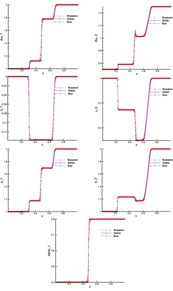
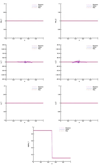
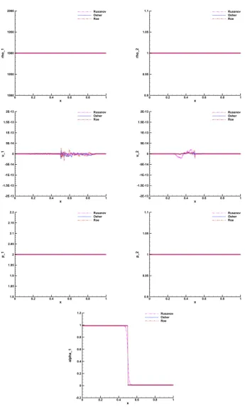
5.1. Numerical results for the two phase RP1 at time t = 0.15 s. . . 67
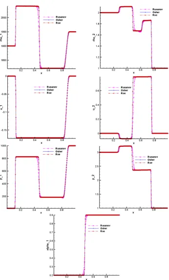
5.2. Numerical results for the two phase RP2 at time t = 0.15 s. . . 68
5.3. Numerical results for the two phase RP3 at time t = 0.15 s. . . 69
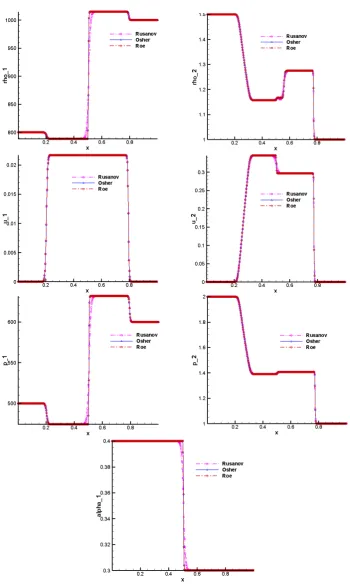
5.4. Numerical results for the two phase RP4 at time t = 0.15 s. . . 70
5.5. Numerical results for the two phase RP4 at time t = 0.15 s. . . 71
5.6. Numerical results for Riemann problems RP1-RP5 (from top to bottom). Left: Solid density ρ1. Right: Gas density ρ2. . . 74
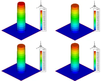
5.7. 3D surface plot for the mixture pressure obtained with a path-conservative Osher-type scheme corresponding to four different mesh sizes listed in Table 5.3. . . 76
5.8. The oscillations of the droplet in time . . . 78
5.9. The oscillations of the droplet in time . . . 78
5.10. Drop falling under gravity effect and break-up. . . 79
5.11. Interface positions in form of volume fraction contour (α2) for a rising 2D bubble. Mesh size is 100×200. . . 80
5.12. Transient flow visualization of a 2D binary drop collision. Mesh size is 200×200. . . 82
5.13. 3D surface plot for the pressure obtained with the HLLEM-type Riemann solver corresponding to four different mesh sizes listed in Table 5.4. . . 84
5.14. Drop falling under gravity effect and break-up. . . 85
5.15. Results for Riemann problem RP1 on the unstructured grid. . . 88
5.16. Results for Riemann problem RP2 on the unstructured grid. . . 89
5.17. Results for Riemann problem RP3 on the unstructured grid. . . 90
5.18. Results for Riemann problem RP4 on the unstructured grid. . . 91
5.19. 2D isentropic vortex problem — Error in logscale as a function of the number of degrees of freedom for the DG schemes tested in table 5.8, from 3rd order up to 10th order of accuracy. . . 95
5.20. Results for Riemann problem RP1. . . 98
5.21. Results for Riemann problem RP2. . . 99
5.22. Results for Riemann problem RP3. . . 100
5.23. Results for Riemann problem RP4. . . 101
5.24. Sketch of the expected behavior for the bubble deformation test starting from an ellipse bubble. A loss of kinetic energy is expected in the dissipative case (green) whereas in an (ideal) non dissipative case the energy remains the same (blue). . . 103
5.25. Laplace law test case — 2D initial ellipse bubble — Kinetic energy as a function of time. . . 104
A.2. Boundary conditions. Ghost cells outside the computational domain are created. . . 109 A.3. Sketch of the boundary conditions. Ghost cell outside the computational
domain is taken, and it is based on a logically connected mesh. . . 110
Symbols
a Speed of sound
c Color function
d Number of space dimensions
i Element index
j Neighbor element index
h Characteristic mesh size
H The enthalpy
M Maximum degree of the reconstruction
n Current time level
n+ 1 Future time level
p Pressure
pI Interface pressure
uI Interface velocity
t Time
T Control volume
u Velocity component in x-direction
v Velocity component in y-direction
w Velocity component in z-direction
x Horizontal direction in the physical system y Lateral direction in the physical system z Vertical direction in the physical system
γ Ratio of specific heats
µ Dynamic viscosity
π Material constant
δij Kronecker symbol
∆t Timestep
ρ Density
α Volume fraction
κ The curvature
σ Surface tension coefficient
λ Velocity relaxation
β Pressure relaxation
g Gravity acceleration
Z Acoustic impedance
Θ Dissipation matrix
ρE Total energy per mass unit
θ Space-time basis function and test function
ψ Space basis function
ξ Horizontal direction in the reference system η Lateral direction in the reference system ζ Vertical direction in the reference system τ Relative time with respect to timelevel tn
τ Viscous shear stress tensor
Ω Computational domain
B Non-conservative nonlinear flux tensor
F Conservative nonlinear flux tensor
I Identity matrix
` Level of refinement
n Element boundary normal vector in space
Ni Neumann neighborhood of element i
r Refinement factor
Q Vector of conserved variables
W Vector of primitive variables
S Algebraic source term
x Physical spatial coordinate vector
˜
x Physical space-time coordinate vector
ξ Reference spatial coordinate vector
˜
ξ Reference space-time coordinate vector
Abbreviations
ADER Arbitrary high order scheme using derivatives ALE Arbitrary-Lagrangian-Eulerian scheme
AMR Adaptive Mesh Refinement
BN Baer-Nunziato
CFD Computational Fluid Dynamics
CG Continuous Galerkin method
CFL Courant-Friedrichs-Levy number
CPU Central processing unit
CSF Continuum surface force
DG Discontinuous Galerkin method
ENO Essentially non-oscillatory
FV Finite Volume
GRP Generalized Riemann problem
GTS Glocal time stepping
LS Level set
LTS Local time stepping
MOOD Multi-dimensional optimal order detection
MUSCL Monotonic Upstream-Centered Scheme for Conservation Laws
NAD Numerical Admissible Criteria
ODE Ordinary differential equation
PAD Physical Admissible Criteria
PLIC Piecewise linear interface reconstruction
PPM Piecewise parabolic method
PDE Partial differential equation
RS Riemann Solver
SPH Smooth Particle Hydrodynamics
TEU Total element updates
TVD Total variation diminishing
VOF Volume of fluid
WENO Weighted essentially non-oscillatory
1. Introduction
1.1. Introduction
Multi-phase flow problems including surface tension and capillary effects are of great in-terest in mechanical, chemical and aerospace engineering. They appear in many industrial processes, such as liquid fuel sprays injected into car, air- and spacecraft engines; mixing processes in chemical engineering; breakup of liquid jets; condensation in nuclear reactors; off-shore engineering and bio-medical applications.
Laboratory experiments and computer simulations are the two main approaches for the study of complex flow problems. So far, most of the knowledge obtained is experimental, but this approach tends to be very complex and is subject to technical limitations when obtaining some measurements. Experimental data tends to include uncertainties that do not allow correct validation of the theory. As a consequence, numerical simulations with modern state of the art methods can help one to understand the complexity involved in these fluid flows more clearly without having to perform time consuming, expensive and complicated experiments. Advances in modern computers combined with advances in nu-merical schemes for the solution of the governing partial differential equations can provide important information, especially at complicated conditions where it can be difficult to extract measurements experimentally. This simulation approach is known as Computa-tional Fluid Dynamics (CFD). In CFD, one has been trying to improve numerical schemes in order to simulate increasingly complex flows with greater accuracy and efficiency. The strategy of computer simulations is presented in Figure 1.1.
Figure 1.1.: The strategy of computer simulations
multi-phase flows.
In the past, many mathematical models and numerical methods have been developed for compressible and incompressible multi-phase flows. A first problem is to determine the location of the interface where the interactions between different fluids take place. Further difficulties arise when shock waves travel across the interface between two fluids. This is due to the fact that the numerical simulation of compressible multi-phase flows is far more complex than the simulation of single phase flows.
The numerical schemes used to solve the interface tracking problem can be classified into three basic categories: tracking methods (moving grid or Lagrangian approach), capturing methods (fixed grid or Eulerian approach) and combined methods.
In general, Lagrangian methods [14] explicitly track the interface of the two fluids via a moving mesh and thus always provide the exact location of the interface. However, mesh-based Lagrangian schemes are typically not suitable for multi-phase flows with complex vortex structures or where a complex merging and separation of the phase interface oc-curs. Thus, a completely different approach for the modeling of multi-phase flows with surface tension is based upon meshless Lagrangian particle schemes, such as the well-known Smooth Particle Hydrodynamics (SPH) method [110]. SPH is well-suited for the simulation of complex interface flows including surface tension, complex vortex flow and separation and merging of the phase interface. The SPH method provides excellent inter-face tracking capabilities, but it is also well known to exhibit several numerical instabili-ties, such as the tensile instability, which require artificial viscosity and other stabilization techniques. It is also important to note that SPH is computationally more expensive than most of the other methods. Furthermore, the method in general lacks even zeroth order consistency with the governing PDE. In recent years, novel SPH techniques have been developed to provide accurate and stable solutions for weakly compressible free surface
flows, see e.g [73, 158].
In Eulerian schemes based on a fixed mesh there are two very popular methods for the capturing of the phase interface, namely the volume of fluid (VOF) method [85] and the level set (LS) method [142, 115, 112]. A combination of VOF and LS proposed in [141, 154] has shown to produce a robust method for flows with complex geometries and interface deformations in the setting of incompressible fluids. The disadvantage of Eulerian methods applied to multiphase flow problems is a significant amount of numerical dissipation, which requires proper interface reconstruction techniques to avoid excessive smearing of the phase boundary and to restore a sharp interface. However, this may become rather cumbersome in complex configurations. The level set method also needs a periodic re-initialization to restore the signed distance function property of the level set function, which requires the additional solution of a Hamilton-Jacobi equation. Furthermore, VOF has difficulties in simulating highly compressible multi-phase flows, hence most of the applications of the VOF method are restricted to the simulation of incompressible fluids. While the VOF method is perfectly conservative, the level-set approach is not. Due to the piecewise linear interface reconstruction (PLIC) used in the VOF context and due to the signed distance function property of the level-set method, both approaches are called
sharp interface methods.
A very recent and completely different method for simulating compressible multi-phase flows is a novel type of model that uses adiffuse interface approach based upon extended hyperbolic systems with stiff relaxation. The basic philosophy of this new type of models is similar to the capturing of discontinuities (shockwaves) in gas dynamics. These methods were presented for the first time by Saurel et al. in [131, 135]. The diffuse interface approach is stabilized by the numerical diffusion provided by the Riemann solver at the interface, and when the mesh size tends to zero, also the interface thickness is approaching zero. Hence, the diffuse interface method is a very interesting alternative approach, and in the limit, also the diffuse interface model tends to a sharp interface representation, but based on a totally different mathematical formulation. The first applications of the diffuse interface method to compressible multi-phase flows with surface tension in two space dimensions have been presented in [121, 21], with a subsequent extension to three space dimensions carried out in [120]. Further recent research on multi-phase flows with surface tension has been presented in [104, 80]. A common problem of all Eulerian methods, i.e. for both sharp and diffuse interface approaches, is the correct calculation of the interface curvature.
dimensions
∂u
∂t +∇ ·F(u) +B(u)· ∇u=S(u), (1.1) whereuis the state vector;F(u) = [f(u),g(u),h(u)] is the flux tensor for the conservative part of the PDE system, with f(u),g(u) andh(u) expressing the fluxes along thex,yand z directions, respectively; B(u) = [B1(u),B2(u),B3(u)] represents the non-conservative
part of the system, written in block-matrix notation. Finally, S(u) is the source term, which may in principle be stiff. When written in quasilinear form, the system (1.1) becomes
∂u
∂t +A(u)· ∇u=S(u), (1.2)
where the matrixA(u) = [A1,A2,A3] =∂F(u)/∂u+B(u) contains both the conservative
and the non-conservative contributions.
The diffuse interface method of Saurel et al. is used for the capturing of the interface. The interface is identified by a function that represents the volume fraction of one of the two phases. The surface tension effects are included by the continuum surface force (CSF) method [20]. Since the CSF approach produces a source term that contains the gradient of the volume fraction function, we propose to treat this term as a non-conservative product rather than a classical volume source term. Recent work on numerical schemes for systems of equations involving non-conservative terms, like Eq. (1.1), includes the family of so-called path-conservative schemes of Castro and Par´es et al. [119, 25, 75, 24] which are based on the theory proposed by Dal Maso, Le Floch and Murat [108] and are a generalization of the usual concept of conservative methods for systems of conservation laws. Note that the weak formulation of the Roe method by Toumi [151] can also be considered as a path-conservative scheme. It has to be clearly stressed that path-conservative schemes have known deficiencies, which have been studied in detail in [2, 26].
In this thesis, various high order path-conservative schemes are used to solve hyperbolic systems of PDEs with non-conservative products and stiff source terms (1.1) in multiple space dimensions. The first one is the second order TVD version of the path-conservative finite volume method. Within this scheme, the smooth part of the CSF source term is integrated like a classical volume source term, while the contributions due to the jumps in the volume fraction function at the element interfaces are naturally taken into account by the path-conservative finite volume scheme. The second one is the extension of high order path-conservative schemes which are used within the ADER approach together with space-time Adaptive Mesh Refinement (AMR) and Discontinuous Galerkin schemes. Due to the path-conservative framework, the surface tension force is naturally included
into the Riemann solver. The physical properties of the interface with curvature κ are solved by the approximate Riemann solver without spurious oscillations near the material interface. Furthermore, the scheme satisfies the Abgrall condition [1] and iswell-balanced
for a circular bubble at rest that obeys the Young-Laplace relation, i.e. where the surface tension force is exactly balanced by the pressure jump across the interface. This well-balancing has been shown via numerical evidence and under the assumption of an exact knowledge of the interface curvature.
Among the numerical methods specifically developed to solve hyperbolic problems, two well-known families are finite volume (FV) methods and Discontinuous Galerkin (DG) schemes. While FV methods are still extremely popular, nowadays, DG methods are becoming increasingly popular. First introduced by Reed and Hill [125] to solve a first order neutron transport equation, DG schemes are applied in different fields, in particular those related to fluid dynamics. In a series of well-known papers, Cockburn and Shu [35, 34, 33, 32, 36] provided a rigorous formal framework of these methods, contributing significantly to their popularization. DG methods are very robust and, among high order numerical methods, they show high flexibility and adaptivity [124]. Moreover, Jiang and Shu [86] proved that DG methods verify an entropy condition leading to nonlinear L2
stability. Unfortunately explicit DG methods have a strong stability limitation, since usually the CFL restriction for these schemes is very severe and the time step in d space dimensions is constrained as ∆t≤ h
d|λmax| 1
2N+1 [66], where h is a characteristic mesh size,
λmax is the maximum signal velocity and N is the degree of the basis polynomial.
unstructured meshes is applied. For various applications of the Baer-Nunziato model the reader is referred to the literature, see e.g. [130, 5, 137, 39, 147, 63, 59, 60]. To our knowledge, this is the first time that a path-conservative scheme has been applied to the problem of surface tension effects in compressible multi-phase flows in the context of the full seven-equation Baer-Nunziato model.
1.2. The compressible Euler and Navier-Stokes equations
for single phase flows
Before going to compressible multi-phase flows, here we briefly recall the compressible single phase flow equations. These equations are the fundamental conservation laws of mass, momentum and energy, which are given below.
Conservation of mass
∂ρ
∂t +∇ ·(ρu) = 0, (1.3)
conservation of momentum ∂ρu
∂t +∇ ·(ρu⊗u)− ∇ ·T=ρg, (1.4)
conservation of energy ∂ ρe+ρ1
2u
2
∂t +∇ ·
ρe+1 2ρu
2
u
+∇ ·q− ∇ ·(T·u) = ρg·u+qs. (1.5)
Here, ρ is the density, u denotes the velocity vector, g is the gravity acceleration, e represents the internal energy, q is the heat flux and qs is the body heating source. The stress tensor is given by T=−p I+τ, wherep represents the fluid pressure, I denotes the unit tensor andτ is the viscous shear stress tensor, respectively. The equations (1.3)-(1.5) are well established flow equations in the literature. They can be either derived from the basic principles of continuum mechanics, or from kinetic gas theory as the asymptotic limit of the Boltzmann equation in the small Knudsen number regime. It is important to mention that if heat flux, viscosity and gravity effects are neglected then these equations reduce to the Euler equations of compressible gas dynamics. The Euler system is a system of non-linear hyperbolic conservation laws that governs the dynamics of compressible materials, such as gases but also liquids or granular materials at high pressures under the assumption that viscous effects can be neglected. We consider the homogeneous three
dimensional Euler system as the following. ∂ρ
∂t +∇ ·(ρu) = 0, ∂ρu
∂t +∇ ·(ρu⊗u) +∇p = 0, ∂E
∂t +∇ ·[u(E+p)] = 0. (1.6) Here, the density ρ, the pressure p and the velocity vector are mentioned in (1.3)-(1.5). The total energy E consists of the internal energy and kinetic energy
E =ρe+ 1 2ρu
2 (1.7)
and the enthalpy H denotes the specific total enthalpy in the form, H = E+P
ρ (1.8)
The system (1.6) has to be closed with an equation of state that relates pressure to density and internal energy e=e(ρ, p). For gases, the ideal gas equation of state is given by
p= (γ−1)
E− 1
2ρu
2
, (1.9)
with γ the adiabatic exponent. For liquid fluids like water, the so-called stiffened gas equation of state can be written by
p= (γ−1)
E− 1
2ρu
2
−γπ, (1.10)
The constantπ characterises the compressibility of the fluid. The speed of sound a is defined by
a2 =
∂p ∂t
s
(1.11)
The speed of sound is a speed at which a disturbance produced by a sound wave travels in a medium. The disturbance is generally very small (a sound wave is not at all as strong as a shock wave), so that the process is considered as isentropic. For a perfect gas, we have the isentropic relationp/γ = constant, and thus,
a2 =γp
1.2.1. 1D Euler equations in conservation form
The one-dimensional Euler equations can be cast in conservative form as follows,
Ut+Fx = 0, (1.13)
where Q= ρ ρu ρE
, F=
ρu ρu2+p
ρuH
. (1.14)
The flux Jacobian reads
A= ∂F
∂U =
0 1 0
(γ−3)u22 (γ−3)u γ−1 γ−1
2 u
2−H
u H + (1−γ)u2 γu
. (1.15)
The matrix A is diagonalizable
A=RΛL (1.16)
where Λ, R, L are the eigenvalues, right and left eigenvectors of the systems (1.13), respectively. They are given by
Λ =
u−a 0 0
0 u 0
0 0 u
, (1.17)
R=
1 1 1
u−a u+a u H−ua u2/2 H+ua
, (1.18)
L= 1 2
γ−1 2a2u2+
u a
−1 2
γ−1
a2 u2+ 1
a
γ−1
2a2
1−γ2−a21u2
γ−1
a2 u −
γ−1
a2 1
2
γ−1 2a2u2−
u a
−1 2
γ−1
a2 u2 − 1
a
γ−1
2a2
, (1.19)
LdU=
dp−ρad u
2a2
−dp−aa22dρ
dp+ρad u
2a2
. (1.20)
where a is the sound speed, considering the ideal equation of state e = p/ρ/(γ−1), the sound speed is given by a = pγp/ρ. In (1.20), the quality dp−aa22dρ corresponds to the
entropy changedsand the corresponding right eigenvector indicates how the conservative variables change due the entropy change,
∂ρ ∂(ρu) ∂(ρE) ∝ 1 u u2/2
. (1.21)
This is often called an entropy wave. The associated eigenvalueugives the speed at which the entropy wave travels: it moves with the local fluid velocity.
1.2.2. 1D Euler equations in physical form
The Euler equations can be written in terms of primitive or physical variables as follows,
Wt+AwWx = 0, (1.22)
where W= ρ u p
, A
w =
u ρ 0
0 u 1
ρ 0 ρa2 u
. (1.23)
Aw is the coefficient matrix of the primitive form of the Euler equations.
Eigenstructure
Aw =RwΛLw (1.24)
with
Λ =
u−a 0 0
0 u 0
0 0 u
, R
w =
−2ρa 1 2ρa
1
2 0
1 2
−ρa2 0 ρa2
, (1.25)
Lw =
0 1 −1
ρa 1 0 −1
a2
0 1 ρa1
, L
wdU=
d u− dpρa
dρ− dpa2
d u+ dpρa
. (1.26)
The second component of (1.25, 1.26) represents the entropy wave, and we thus find
∂ρ ∂u ∂p ∝ 1 0 0
. (1.27)
From (1.27), the density changes due to the entropy wave; the velocity and the pressure are not effected.
Change of variables
dU= ∂U
∂WdW, dW= ∂W
where ∂U ∂W =
1 0 0
u ρ 0
u2/2 ρ u 1/(γ−1)
, (1.29)
∂W ∂U = ∂U ∂W −1 =
1 0 0
−u ρ
1
ρ 0
(γ−1)u2/2 −(γ−1)u γ−1
. (1.30)
The coefficient matrix Aw is related to the Jacobian matrix
Aof the conservative form by
Aw = ∂W
∂UA ∂U
∂W. (1.31)
Hence, the eigenvectors are given by
L=Lw∂W
∂U, R= ∂U ∂WR
w. (1.32)
1.3. Baer Nunziato equations
In general, averaging is a well established mathematical tool to derive multi-phase flow models from the single-phase equations. There are several types of averaging procedures which can be classified into four categories, such as time averaging [106], volume averaging [157], time and volume averaging [43], and ensemble averaging [42]. These procedures have been used by Saurel and Abgrall in [130] to obtain a seven equation model consisting of phase-specific mass, momentum, and energy conservation equations; one phase is consid-ered to be consisting of an ensemble of particles embedded in a carrier fluid. A transport equation for the volume fraction or color function (of one of the phases) completes the system of equations. The main difference between Baer and Nunziato’s work and that of Saurel and Abgrall is related to the use of relaxation terms and the definition of the interface velocity and pressure. Saurel and Abgrall introduced the notion of relaxation parameters enabling a wider application of the seven equation model. The approach by Saurel and Abgrall [130] has been shown to apply to both interface as well as homogenous two-phase flows.
In this section, multi-phase flows will be presented in the form of the original Baer-Nunziato equations [6]. Two phase flows can be obtained by applying the single-phase flow equations on both sides of the interfaces. The balance laws for each phase are similar to those for an isolated gas, i.e., each phase can be defined by a system of compressible Euler equations plus non-conservative terms (called nozzling terms) which take into account
the interphase exchange of pressure and velocity. As mentioned in the literature, there are several difficulties related to the non-conservation property of the balance equations. Hence, the design of efficient algorithms or novel methods for solving the equations has been a very challenging problem. Since the non-conservative terms do not represent fluxes, they have to be integrated as source terms. In some studies, for simple schemes, the nozzling terms are ignored to get numerical stability and non-oscillatory behavior of numerical methods [79, 117]. However, to guarantee that the entropy inequality is satisfied [137] these terms are required. Similar to the shallow-water equations, where a numerical scheme must preserve the lake-at-rest solution, a two-phase flow with initially uniform velocity and pressure should remain as such for all times, as derived by Abgrall in [1]. In recent years some other seven-equation models have been suggested by [131] and Romenski et al [128]. However, it has also been reduced to a five equation model in [89, 113, 134, 93].
1.3.1. The seven-equation Baer-Nunziato model with relaxation,
surface tension, viscosity and gravity effects
In this thesis we consider the full seven-equation Baer-Nunziato model for compressible two-phase flows including surface tension and gravity effects. The original model has been described in [6] and has been successively modified in [131]. The original Baer-Nunziato model has been proposed for the description of the deflagration-detonation transition in high-energy reactive materials. The full model with relaxation terms, gravity, viscosity and surface tension effects is given by the following non-conservative system:
∂
∂t(α1ρ1) +∇ ·(α1ρ1u1) = 0, ∂
∂t(α1ρ1u1) +∇ ·(α1(ρ1u1⊗u1+p1I−τ1))−pσ∇α1 = α1ρ1g−λ(u1−u2), ∂
∂t(α1ρ1E1) +∇ ·[α1((ρ1E1+p1)I−τ1)·u1]−pσuI · ∇α1 = α1ρ1g·u1−λ (u1−u2)·uI−β pI(p1−p2),
∂
∂t(α2ρ2) +∇ ·(α2ρ2u2) = 0, ∂
∂t(α2ρ2u2) +∇ ·(α2(ρ2u2⊗u2+p2I−τ2))−pI∇α2 = α2ρ2g+λ(u1−u2), ∂
∂t(α2ρ2E2) +∇ ·[α2((ρ2E2+p2)I−τ2)·u2]−pIuI · ∇α2 = ρ2g·u2+λ (u1−u2)·uI+β pI(p1−p2),
∂
In the above system αj is the volume fraction of phase number j, with j ∈ {1,2}, and the constraint α1+α2 = 1. The constraint immediately yields the relation∇α2 =−∇α1.
Furthermore, ρj, uj, pj and ρjEj represent the density, the velocity vector, the pressure and the total energy per unit mass for phase number j, respectively. The viscous stress tensor τj of phase number j that is supposed to be a Newtonian fluid under Stokes’ hypothesis is given by
τj =µj ∇uj +∇uTj
− 2
3µj(∇ ·uj) I, (1.34) where T represents the transpose operator,µj is the dynamic viscosity of fluid j and Iis the identity matrix. The relaxation parameter for the interphase drag is given by λ, the parameter governing the pressure relaxation is denoted byβ andgis the vector of gravity acceleration. Furthermore, the interface pressure of phase 1 that includes the surface tension effect is abbreviated with pσ =pI−σκ, whereσ is the surface tension coefficient and κ is the interface curvature.
The model (1.33) is closed by the stiffened gas equation of state (EOS) for each phase ej = pj+γjπj
ρj(γj −1)
, (1.35)
and the definition of the total energy density ρjEj =ρjej +
1 2ρju
2
j, (1.36)
where γj is the ratio of specific heats and πj is a material constant. In this work, we choose uI = u1 for the interface velocity and the interface pressure is assumed to be pI = p2. This corresponds to the original choice proposed in [6]. Other options are possible,
see for example in [131], uI is defined as velocity of the center of mass and pI is defined by mixture pressure and they are given as follows
uI =
α1ρ1u1+α2ρ2u2
α1ρ1+α2ρ2
, pI =α1p1+α2p2. (1.37)
Moreover, other closure relations were derived in [132] which are given by pI =
Z1p2+Z2p1
Z1+Z2
+ Z1Z2 Z1+Z2
∇α1
|∇α1|
·(u2−u1) (1.38)
uI =
Z1u2+Z2u1
Z1+Z2
+ Z1Z2 Z1+Z2
∇α1
|∇α1|
·(p2−p1) (1.39)
Here, Zk represents the acoustic impedance with
Zk =ρkck, k = 1,2, (1.40)
whereck is the speed of sound defined by
c2k = pk
ρ2 k
−∂ek
∂ρk
∂ek
∂ρk
pk
k = 1,2. (1.41)
As mention above (1.33), the interaction between the two fluids is given by the non-conservative terms as well as by the pressure and velocity relaxation terms. The pressure relaxation termsβ(p1−p2) and±βpI(p1−p2) appear in the volume fraction equations and
energy equations, respectively. Pressure relaxation and interface pressure condition were mentioned by Saurel and Abgrall in [131]. These terms are important in many aspects, for example, they control the relaxation phenomena behind the shock and pressure waves. Also, these terms are responsible for the interfacial pressure condition between the fluids and this condition expresses the equality of pressure.
The velocity relaxation terms±λ(u1−u2) appear in the momentum equations and the
terms ±λuI(u1−u2) in the energy equations, where λ > 0 is the velocity relaxation
parameter. This parameter gives the rate at which the velocities relax to a common value. Such terms are used to model the drag force. The drag force is because of the imbalance of the pressure and due to the viscous stresses of an elementary particle, i.e. solid particle, bubble or droplet. From experiments the relation for the drag force is defined as
Fdrag =λ(u1−u2)). (1.42)
The parameterλdepends upon the geometric parameters of the particle and the Reynolds number which describe the nature of the flow. Note that in the case λ → +∞ and β → +∞ the system instantaneously relaxes to the mechanical equilibrium equations if the surface tension and viscosity effects are ignored. As mentioned in [133], pressure and velocity relaxation procedures are used in the seven-equation model to make it valid for several different applications and a large variety of problems like interface flows, deto-nation, and cavitation in multi-phase flows. According to [20], the surface force per unit volume reads
FS =σκ
∇Φ
[Φ], (1.43)
where σ is the surface tension coefficient, which depends on the kind of fluids under consideration. Φ is a color function, e.g. a volume fraction, and according to the discussion in [121] Φ is taken as the liquid volume fraction in the following, i.e. Φ =α1. The symbol
approximated as an equivalent, distributed volume force. This is exactly the approach of the continuum surface force (CSF) method introduced by Brackbill et al. [20]. Some numerical results obtained with the CSF approach can be seen in [107, 114, 142, 152]. For a steady circular bubble in equilibrium, the pressure jump across the interface of two different fluids is given by the Young-Laplace equation which will be presented in section 1.4. The curvature κ is defined in terms of the normal vector to the phase boundary m as follows:
κ=∇ ·m=∇ ·
∇
α1
k∇α1k
. (1.44)
In (1.33), the surface tension terms appear only in the momentum and the energy equation of the liquid phase (phase number 1). The interactions of the two phases are given by the relaxation source terms, which are purely algebraic, and by the non-conservative terms involving the gradient of the volume fractions (nozzling terms). These non-conservative terms directly affect the wave structure of the Baer-Nunziato system. The system (1.33) can be written in the following compact matrix-vector notation:
∂Q
∂t +∇ ·F(Q,∇Q) +B(Q, κ)· ∇Q=S(Q), (1.45)
with the state vector Q = Q(x, t), the vector of spatial coordinates x = (x, y) and the nonlinear flux tensor F(Q,∇Q) = (f,g) that depends on the state vector and its gradient, to take into account also viscous effects. The purely non-conservative terms are represented by B(Q, κ)· ∇Q, while the algebraic source terms like relaxation and gravity effects are contained inS(Q). We furthermore introduce the symbolA(Q, κ) =∂F/∂Q+ B(Q, κ), which groups the Jacobian of the flux tensor with the non-conservative terms. In the description of system (1.45), the local curvatureκ is considered as a parameter. In the absence of viscous terms, the system (1.45) is called hyperbolic if for all unit normal vectors n with knk= 1 the matrix
A(Q, κ,n) = A(Q, κ)·n=R(Q, κ,n)Λ(Q, κ,n)R−1(Q, κ,n) (1.46)
is diagonalizable with Λ = diag(λ1, λ2, . . . λ9) real and a full set of linearly independent
right eigenvectors R.
1.3.2. Eigenstructure of the Baer-Nunziato model in 1D
If we ignore the viscous effects, the gravity and relaxation terms in (1.33), the Baer-Nunziato system with surface tension reads in one space dimension as follows:
∂(α1ρ1)
∂t +
∂(α1ρ1u1)
∂x = 0, ∂(α1ρ1u1)
∂t +
∂(α1(ρ1u1u1+p1))
∂x −pσ ∂α1
∂x = 0, ∂(α1E1)
∂t +
∂(α1u1(E1+p1))
∂x −pσuI ∂α1
∂x = 0, ∂(α2ρ2)
∂t +
∂(α2ρ2u2)
∂x = 0, ∂(α2ρ2u2)
∂t +
∂(α2(ρ2u2u2+p2))
∂x +pI ∂α1
∂x = 0, ∂(α2E2)
∂t +
∂(α2u2(E2+p2))
∂x +pIuI ∂α1
∂x = 0, ∂α1
∂t +uI ∂α1
∂x = 0. (1.47)
We can rewrite system (1.47) in a more compact non-conservative form (1.48), given below,
∂Q ∂t +
∂f(Q)
∂x +B(Q, κ) ∂Q
∂x = 0, x∈Ω⊂R, t ∈R
+
0, (1.48)
whereQ is the vector of state variables,f(Q) is the flux vector for the purely conservative part of the system and B(Q) contains the purely non-conservative part of the system. The quantities Q, f(Q) andB(Q, κ) are defined as,
Q=
α1ρ1
α1ρ1u1
α1E1
α2ρ2
α2ρ2u2
α2E2
α1
, f(Q) =
α1ρ1u1
α1(ρ1u1u1+p1)
α1u1(E1+p1)
α2ρ2u2
α2(ρ2u2u2+p2)
α2u2(E2+p2)
0 , (1.49)
B(Q, κ) =
0 0 0 0 0 0 0
0 0 0 0 0 0 −pσ 0 0 0 0 0 0 −pσuI
0 0 0 0 0 0 0
0 0 0 0 0 0 pI 0 0 0 0 0 0 uIpI 0 0 0 0 0 0 uI
System (1.47) can also be written in the following quasilinear form ∂Q
∂t +A(Q, κ) ∂Q
∂x = 0, (1.51)
with the system matrix given byA(Q, κ) = ∂f(Q)/∂Q+B(Q, κ), where we have dropped the dependence on the normal vector n for the 1D case. After having introduced the vector of primitive variables W = (ρ1, u1, p1, ρ2, u2, p2, α1)T, we can rewrite the
quasi-linear system (1.52) in terms of the primitive variables as ∂W
∂t +C(W, κ) ∂W
∂x = 0, (1.52)
with the system matrix C(W, κ) = ∂W
∂Q A(Q(W), κ) ∂Q
∂W, and
∂W ∂Q =
∂Q ∂W
−1
. (1.53)
In one space dimension the matrix C(W, κ) and the Jacobian ∂∂WQ read as follows:
C(W, κ) =
u1 ρ1 0 0 0 0 0
0 u1 ρ1
1 0 0 0
p1−p2+σκ
α1ρ1
0 α2
1ρ1 u1 0 0 0 0
0 0 0 u2 ρ2 0 ρ2(u1
−u2)
α2
0 0 0 0 u2 ρ12 0
0 0 0 0 α2
2ρ2 u2
(u1−u2)α22ρ2
α2
0 0 0 0 0 0 u1
, (1.54) ∂Q ∂W =
α1 0 0 0 0 0 ρ1
α1u1 α1ρ1 0 0 0 0 ρ1u1 1
2α1u 2
1 α1ρ1u1 γ1α−11 0 0 0 ρ1E1
0 0 0 α2 0 0 −ρ2
0 0 0 α2u2 α2ρ2 0 −ρ2u2
0 0 0 12α2u22 α2ρ2u2 γ2α−21 −ρ2E2
0 0 0 0 0 0 1
. (1.55)
The sound speeds of the liquid and the gas phases are given by
aj =
s
γj(pj+πj) ρj
. (1.56)
The eigenvalues of the matrixC(W, κ) are then given byΛ= diag(u1−a1, u1, u1+a1, u2−
a2, u2, u2+a2, u1). It is important to notice that the eigenvalues of the system (1.47) with
and without the surface tension effect are the same. The right and left eigenvector matrix corresponding to these eigenvalues are,
R=
−ρ1
a1 1
ρ1
a1 0 0 0 0
1 0 1 0 0 0 0
−ρ1a1 0 ρ1a1 0 0 0 −(a22−u21+ 2u1u2−u22)α2b
0 0 0 −ρ2
a2 1
ρ2
a2 −ρ2(u 2
1−2u1u2+u22)α1
0 0 0 1 0 1 −(u1−u2)α1α22
0 0 0 −a2ρ2 0 a2ρ2 −a22α1p2(u21−2u1u2+u22)
0 0 0 0 0 0 α2(a22−u21−2u1u2−u22)α1 , and
R−1 =
0 12 − 1
2ρ1a1 0 0 0 −
p1−p2+σκ 2ρ1a1α1
1 0 −1
a2
1 0 0 0 −
p1−p2+σκ
a2 1α1
0 1 2
1
2ρ1a1 0 0 0
p1−p2+σκ 2ρ1a1α1
0 0 0 0 12 − 1
2a2ρ2
(u1−u2)a2 2(a2−u2+u1)α2
0 0 0 1 0 −1
a2
2 0
0 0 0 0 12 2a1
2ρ2
(u1−u2)a2 2(a2+u2−u1)α2
0 0 0 0 0 0 α 1
2(a22−u21+2u1u2−u22)α1 , (1.57)
withb= (p1−p2+σκ). MatrixC(W, κ) can thus be written asC(W, κ) =RΛR−1 and
therefore one immediately also gets the eigenstructure of the matrix A(Q, κ) as
A(Q, κ) =
∂Q ∂WR Λ
R−1 ∂W ∂Q
.
Figure 1.2.: The wave structure of an idealized Riemann problem for the seven-equation multi-phase flow model.
1.4. Young-Laplace Equation
In the model (1.33), the surface tension is constructed as boundary values present only at the interface, so that discontinuities or abrupt changes occur in the various variables. The phase interface can be resolved using different methods by deriving the types of the jump conditions. As discussed in [138, 106], these jump conditions actually contain the exchange of mass, momentum and energy across the interface; the properties of the phase interface are very similar the other phases in multi-phase flow systems. The jump conditions are given by mass jump
[ρ(u−ui)]·n, (1.58)
momentum jump
[ρu(u−ui) +T]·n=mσi, (1.59) energy equation
ρ
e+1 2u
2
u(u−ui) +T·u−q
·n=eσi, (1.60) where for any variablekat both sides of the interface, the jump is defined as [k] =k+−k−.
In (1.58) - (1.60), ui represents the velocity of the interface,nis the outward pointing unit normal vector. The interactions at the phase interface are affected by the surface tension σ and energy related with the phase interface eσ
i. Here we only consider the condition (1.59), in the case of non-equilibrium of a circular bubble, the pressure gradient and the capillary forces at the interface are unbalanced, giving rise to a nonzero velocity field
in the vicinity of the interface that tends to reshape an initially elliptical bubble into a circular one. Otherwise, for a steady circular bubble in equilibrium, the pressure jump across the interface of two fluids is given by Young-Laplace Equation as
p1 −p2 = ∆p=σκ, (1.61)
see [74, 13]. The curvature κ is defined in (1.44), andσ is the surface tension coefficient of the fluid between the gaseous and the liquid phase. The surface tension coefficientσ is assumed to be a positive constant and it also is dependent on the properties of the fluid.
1.5. Overview of the thesis
2. Path-conservative Finite Volume
Schemes
In this chapter we are going to discuss the numerical methods, which are applied for solving the equations of compressible multi-phase flows with surface tension. First, we describe the general framework of finite volume schemes for hyperbolic conservation laws, second we extend to path-conservative finite volume schemes on Cartesian and unstructured meshes, as well as a finite volume scheme with time-accurate local time stepping (LTS) on unstructured grids. Finally, the curvature computation is discussed.
2.1. Finite volume methods
Assuming the family of hyperbolic PDEs is written in the differential form of conservation laws. In Cartesian coordinates and in three space dimensions, it is written as
∂u ∂t + ∂f ∂x + ∂g ∂y + ∂h
∂z = 0, (2.1)
where u is the vector of conserved variables, f,g,h are the flux vectors in the direction of x, y, z, respectively. In order to obtain the finite volume formulation of (2.1), we discretize the computational domain Ω in space-time control volumes defined as Iijk =
Iijk×[tn, tn+ ∆t] =
h
xi−1 2, xi+
1 2 i
×hyi−1 2, yi+
1 2 i
×hzi−1 2, zi+
1 2 i
×[tn, tn+ ∆t], with ∆x i = xi+1
2 −xi−
1
2,∆yi =yi+
1
2 −yi−
1
2,∆zi =zi+
1
2 −zi−
1
2 and ∆t=t
n+1−tn. After integration of (2.1) over a space-time control volume Iijk one obtains the following finite volume formulation:
¯
unijk+1 = ¯unijk− ∆t
∆xi
h
fi+1
2,j,k−fi− 1 2,j,k i − ∆t ∆yj h
gi,j+1
2,k−gi,j−
1 2,k i − ∆t ∆zk h
hi,j,k+1
2 −hi,j,k− 1 2 i , (2.2) where ¯
unijk = 1 ∆xi
1 ∆yj
1 ∆zk
xi+ 1
2 Z
xi−1 2
yj+ 1
2 Z
yj−1 2
zk+ 1
2 Z
zk−1 2
is the spatial average of the solution in the element Iijk at the time tn, while fi±1 2,j,k,
gi,j±1
2,k, and hi,j,k± 1
2 are the average fluxes along each Cartesian direction and in time as
follows:
fi±1
2,j,k =
1 ∆t 1 ∆yj 1 ∆zk
tn+1
Z
tn
yj+ 1
2 Z
yj−1 2
zk+ 1
2 Z
zk−1 2
˜fu(x i±1
2,j,ky, z, t)
dz dy dt, (2.4)
gi,j±1
2,k =
1 ∆t 1 ∆xi 1 ∆zk
tn+1 Z
tn
xj+ 1
2 Z
xj−1 2
zk+ 1
2 Z
zk−1 2
˜ g
u(x, yi,j±1
2,k, z, t)
dz dx dt, (2.5)
hi,j,k±1
2 = 1 ∆t 1 ∆xi 1 ∆yj
tn+1 Z
tn
xj+ 1
2 Z
xj−1 2
yk+ 1
2 Z
yk−1 2
˜
hu(x, y, zi,j,k±1 2, t)
dy dx dt. (2.6)
2.2. Conservation laws in generalized coordinates
In general computations, geometries are not simple and, therefore, the grids associated with these geometries are also not trivial. So, to account for these non-uniformities, modi-fications to the above described algorithm become necessary, one considers the coordinate transformation:
ξ =ξ(x, y, z), η=η(x, y, z), ζ =ζ(x, y, z), (2.7) which defines a map between the physical coordinates (x, y, z) and the computational (or generalized) coordinates (ξ, η, ζ). It maps a curvilinear grid in the physical space to a Cartesian grid in the computational space. Computing the first order derivative of any variable φ with regard to x, y and z, respectively is done using the chain rule according to the following formulae:
∂φ ∂x = ∂ξ ∂x ∂φ ∂ξ + ∂η ∂x ∂φ ∂η + ∂ζ ∂x ∂φ
∂ζ, (2.8)
∂φ ∂y = ∂ξ ∂y ∂φ ∂ξ + ∂η ∂y ∂φ ∂η + ∂ζ ∂y ∂φ
∂ζ, (2.9)
∂φ ∂z = ∂ξ ∂z ∂φ ∂ξ + ∂η ∂z ∂φ ∂η + ∂ζ ∂z ∂φ
∂ζ. (2.10)
The metric coefficients such as ∂x∂ξ,∂ξ∂y,∂ξ∂z, ∂η∂x,∂y∂η,∂η∂z, and ∂ζ∂x,∂ζ∂y,∂ζ∂z are given by, ∂ξ
∂x =J(yηzζ −yζzη), ∂ξ
∂y =J(xζzη −xηzζ) ∂ξ
∂z =J(xηyζ−xζyη) (2.11)
∂η
∂x =J(yζzξ−yξzζ), ∂η
∂y =J(xξzζ−xζzξ) ∂η
∂z =J(xζyξ−xξyζ) (2.12) ∂ζ
∂x =J(yξzη−yηzξ), ∂ζ
∂y =J(xηzξ−xξzη) ∂ζ
∂z =J(xξyη−xηyξ) (2.13) where
J= 1
xξ(yηzζ−yζzη)−xη(yηzζ−yζzη)−xζ(yξzη −yηzξ)
, (2.14)
which can be used to compute spatial derivatives in (x, y, z) from variables mapped on to (ξ, η, ζ). The set of these formulae of the derivatives xξ, xη, xζ, yξ, yη, yζ and zξ, zη, zζ are given by
xξ =
xi+1,j,k−xi−1,j,k
2 , xη =
xi,j+1,k−xi,j−1,k
2 , xζ =
xi,j,k+1−xi,j,k−1
2 , (2.15)
yξ =
yi+1,j,k−yi−1,j,k
2 , yη =
yi,j+1,k −yi,j−1,k
2 , yζ =
yi,j,k+1−yi,j,k−1
2 , (2.16)
zξ =
zi+1,j,k−zi−1,j,k
2 , zη =
zi,j+1,k−zi,j−1,k
2 , zζ =
zi,j,k+1−zi,j,k−1
2 . (2.17)
For more details, see [3, 4]. From the above transformations, the differential form of the conservation law (2.1) will be given as
∂u∗ ∂t +
∂f∗ ∂ξ +
∂g∗ ∂η +
∂h∗
∂ζ = 0, (2.18)
where
u∗ = u
J (2.19)
f∗ = 1 J
f∂ξ ∂x +g
∂ξ ∂y +h
∂ξ ∂z
(2.20)
g∗ = 1 J
f∂η ∂x +g
∂η ∂y +h
∂η ∂z
(2.21)
f∗ = 1 J
f∂η ∂x +g
∂ζ ∂y +h
∂ζ ∂z
. (2.22)
2.3. Total-Variation-Diminishing Schemes
The most well known and one of the most successful schemes for the numerical solution of nonlinear systems of conservation laws is the method of Godunov. Here, data are repre-sented by piecewise constant cell averages, and these piecewise constant data are also used to compute the numerical fluxes. Since the original Godunov method is only first-order accurate, it is too diffusive. Therefore, we need to develop high order schemes for hyper-bolic problems. One of the main drawbacks of high order schemes are spurious oscillations at shock waves and discontinuities, the so-called Gibbs’ phenomenon. According to the Godunov theorem, there are no better than first order accurate linear monotone schemes. This means, that in order to circumvent the theorem, high order schemes for conservation laws must be necessarily nonlinear, to overcome the drawbacks of high order schemes and achieve high order of accuracy, one of the most popular schemes is the MUSCL scheme, which is both monotonicity preserving and higher than first order accurate. This scheme was first proposed by Kolgan [90] and later independently rediscovered by van Leer [153]. This scheme makes use of piecewise linear data inside every computational cell, while first order finite volume schemes rely only on a piecewise constant data representation see Figure 2.1. In this section we will briefly introduce the scheme, which relate to a
Figure 2.1.: Piecewise constant data representation in a first order finite volume scheme (left) and piecewise linear data (right) in the second order finite volume MUSCL scheme.
linear polynomial, variations and oscillations in nonlinear systems, that is the so-called Total Variation Diminishing (TVD) of property Harten et al [83], for a general overview, the reader is referred to [148, 96]. The total variation for a scalar conservation law of a discrete function q,
T V (q) =
Z
|∂q
∂x|dx, (2.23)
does not increase. With the definition of Harten, the total variation (TV) of a discrete functionqhn is given as,
T V (qhn) =
∞
X
i=−∞
|qin+1−qin|, (2.24) with qn
i → const. for i → ±∞. A numerical method
qin+1 =H qin−l, . . . , qin+r (2.25) is called TVD if
T V qnh+1≤T V (qnh). (2.26) If a conservative scheme is TVD, then it converges to the weak solution. A piecewise linear polynomial reconstruction for celli reads
Pin(x) = Qni + ∆Q n i
∆x (x−xi), (2.27)
where Qn
i is the Godunov cell average and the slope
∆Qn
i
∆x must be properly defined in order to ensure the TVD property. This is usually achieved at the aid of so-called slope limiters.
In (2.24) we can see that oscillations in the computational results will increase the total variation. So numerical schemes for which the total variation of the solution satisfies the condition in (2.26) are called TVD schemes.
2.4. Path-conservation Finite volume schemes
Here, we recall the path-conservative finite volume schemes of Par´es and Castro [119, 25] that we are going to use in order to discretize the non-conservative governing PDE system (1.45). We also briefly summarize the new generalized Osher-type Riemann solver (DOT) presented in [64, 65], as well as the more popular path-conservative Rusanov and Roe schemes. For all three methods, we will, however, rely on the numerical evaluation of the path integral along the straight line segment path by using high Gauss-Legendre quadrature rules according to [64, 65, 63]. The method is implemented inside a classical second order accurate high resolution TVD framework.
2.4.1. Path-conservation Finite volume schemes for the 2D
Baer-Nunziato equaion on the Cartesian meshes
The computational domain Ω is discretized by a set of non-overlapping control volumes Ti,j = [xi−1
2, xi+ 1
2]×[yj− 1 2, yj+
1
of constant width ∆x=xi+1
2 −xi−
1
2 and ∆y =yj+ 1
2 −yj+
1
2, respectively. We denote the
spatial barycenter of Ti,j with xi,j = (xi, yj) =
1 2(xi−1
2 +xi+
1 2),
1 2(yj−1
2 +yj+
1 2)
. The time step is denoted by ∆t =tn+1−tn. The cell averages at time tn on T
i,j are defined as usual by
Qni,j = 1 ∆x∆y
xi+ 1
2 Z
xi−1 2
yj+ 1
2 Z
yj−1 2
Q(x, y, tn)dy dx, (2.28)
from which a second order TVD scheme in space can be constructed by using the following nonlinear slope reconstruction:
∇Qni,j = ∂xQ n i,j ∂yQni,j
!
=
minmodQ
n
i+1,j−Qni,j
∆x ,
Qn
i,j−Qni−1,j ∆x
minmodQ
n
i,j+1−Qni,j
∆y ,
Qn
i,j−Qni,j−1 ∆y
, (2.29)
with the classical minmod slope limiter detailed, for example, in [148], where
minmod (a, b) =
a if |a| ≤ |b| and ab >0, b if |a|>|b| and ab >0, 0 ifab≤0.
(2.30)
A second order MUSCL-type scheme in time can then be obtained by the following ap-proximation of the first derivative of Q in time, which is based on a discrete form of the governing PDE as follows:
∂tQni,j = −f Q
n
i,j+ ∆2x∂xQ
n
i,j,∇Qni,j
−f Qn
i,j− ∆2x∂xQ
n
i,j,∇Qni,j
∆x
−g Q
n i,j +
∆y
2 ∂xQ
n
i,j,∇Qni,j
−g Qn i,j −
∆y
2 ∂yQ
n
i,j,∇Qni,j
∆y
−B Qni,j, κni,j· ∇Qni,j+S Qni,j. (2.31)
The resulting piecewise linear space-time reconstruction polynomial inside cell Ti,j then reads
Q(x, t)|T
i,j =Q
n
i,j +∇Q n
i,j·(x−xi,j) +∂tQni,j (t−t
n). (2.32)
The second order TVD version of the path-conservative finite volume method is now obtained by using the piecewise linear data representation (2.32) and by integration of the governing PDE system over the space-time control volume [xi−1
2, xi+ 1
2]×[yj− 1 2, yj+
1
2]×
[tn, tn+1]:
Qni,j+1 = Qni,j − ∆t
∆x
fi+1
2,j−fi− 1 2,j − ∆t ∆y
gi,j+1
2 −gi,j−
1 2 −∆t ∆x
Di+1
2,j+Di−
1 2,j − ∆t ∆y
Di,j+1
2 +Di,j−
1 2
−∆tBQn+
1 2
i,j , κ n i,j
· ∇Qni,j+ ∆tSQn+
1 2
i,j
, (2.33)
with Qn+
1 2
i,j = Q(xi,j, tn+
1
2). In (2.33), the f
i±1
2,j and gi,j±
1
2 denote the numerical fluxes
for the purely conservative and the viscous part of the PDE, while the terms Di±1
2,j and
Di,j±1
2 take into account the jump of the piecewise linear data reconstruction (2.32) at
the element interfaces. The term BQn+
1 2
i,j , κni,j
· ∇Qn
i,j accounts for the smooth part of the non-conservative product and SQn+
1 2
i,j
is an explicit discretization of the algebraic source term.
The numerical flux fi+1
2,j inx direction is given by
fi+1
2,j =
1 2
fQ+i+1 2,j
,∇Qni+1 2,j
+fQ−i+1 2,j
,∇Qni+1 2,j
− 1
2Θi+12,j
Q+i+1 2,j
−Q−i+1 2,j
, (2.34) where Θi+1
2,j > 0 is a positive definite dissipation matrix that depends on the
approxi-mate Riemann solver to be used and that will be defined later. Furthermore, Q−i+1 2,j
= Q(x−i+1
2
, yj, tn+
1
2) and Q+
i+12,j = Q(x
+
i+12, yj, t
n+12) denote the boundary-extrapolated
val-ues taken at the half time level at the element interface from the left and the right, respectively, while ∇Qni+1
2,j
denotes the unlimited gradient at the edge that is used for the computation of the viscous fluxes and that is defined as the average of the corner gradients ∇Qni+1
2,j± 1 2
as follows:
∇Qni+1 2,j
= 1 2
∇Qni+1 2,j+
1 2
+∇Qni+1 2,j−
1 2
with
∇Qni+1 2,j+
1 2
= 1 2
Qn
i+1,j+1−Qni,j+1
∆x +
Qn
i+1,j−Qni,j
∆x
Qn
i+1,j+1−Qni+1,j
∆y +
Qn
i,j+1−Qni,j ∆y
!
. (2.35)
The jump terms due to the non-conservative product are simply defined as
Di±1
2,j =
1 2
1 Z
0
Bψ(Q−i±1 2,j
,Q+i±1 2,j
, s), κni±1 2,j
·ni±1 2,jds
≈ 1
2
X
l ωlB
ψ(Q− i±1
2,j
,Q+ i±1
2,j
, sl), κni±1 2,j
·ni±1
2.4.2. Curvature computation
The surface tension effect is naturally included inside the non-conservative terms of system (1.33). Since the term pσ in system (1.33) contains the curvature κ, defined according to (1.44), we first need to compute the gradient of the volume fraction function at the beginning of each time step at the vertices of the two dimensional Cartesian grid, i.e. at the location xi+1
2,j+ 1
2, while the cell centers are located atxi,j. By using this vertex-based
staggering, according to Perigaud et al [121], the unlimited corner gradient of the volume fraction function is computed as follows:
∇αn1,i+1 2,j+
1 2
= 1 2
αn1,i+1,j+1−αn1,i,j+1
∆x +
αn1,i+1,j−αn1,i,j
∆x
αn
1,i+1,j+1−