Function, Interactions, Evolution
Stefano Teso
2013/12/19
International Doctorate School in Information and
Communication Technologies
DIT - University of Trento
Advisor:
Abstract
In recent years, the field of Statistical Relational Learning (SRL) [1, 2] has produced new, powerful learning methods that are explicitly designed to solve complex problems, such as collective classification, multi-task learning and structured output prediction, which natively handle relational data, noise, and partial information. Statistical-relational methods rely on some First-Order Logic as a general, expressive formal language to encode both the data instances and the relations or constraints between them. The latter encode background knowledge on the problem domain, and are use to restrict or bias the model search space according to the instructions of domain experts. The new tools developed within SRL allow to revisit old computational biology problems in a less ad hoc fashion, and to tackle novel, more complex ones. Motivated by these developments, in this thesis we describe and discuss the application of SRL to three important biological problems, highlighting the advantages, discussing the trade-offs, and pointing out the open problems.
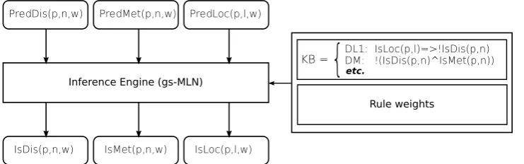
In particular, in Chapter 3 we show how to jointly improve the outputs of multiple correlated predictors of protein features by means of a very gen-eral probabilistic-logical consistency layer. The logical layer — based on grounding-specific Markov Logic networks [3] — enforces a set of weighted first-order rules encoding biologically motivated constraints between the pre-dictions. The refiner then improves the raw predictions so that they least violate the constraints. Contrary to canonical methods for the prediction of protein features, which typically take predicted correlated features as in-puts to improve the output post facto, our method can jointly refine all predictions together, with potential gains in overall consistency. In order to showcase our method, we integrate three stand-alone predictors of corre-lated features, namely subcellular localization (Loctree[4]), disulfide bonding state (Disulfind[5]), and metal bonding state (MetalDetector[6]), in a way that takes into account the respective strengths and weaknesses. The ex-perimental results show that the refiner can improve the performance of the underlying predictors by removing rule violations. In addition, the proposed method is fully general, and could in principle be applied to an array of
heterogeneous predictions without requiring any change to the underlying software.
In Chapter 4 we consider the multi-level protein–protein interaction (PPI) prediction problem. In general, PPIs can be seen as a hierarchical process occurring at three related levels: proteinsbind by means of specific domains, which in turn form interfaces through patches of residues. Detailed knowl-edge about which domains and residues are involved in a given interaction has extensive applications to biology, including better understanding of the bind-ing process and more efficient drug/enzyme design. We cast the prediction problem in terms of multi-task learning, with one task per level (proteins, domains and residues), and propose a machine learning method that collec-tively infers the binding state of all object pairs, at all levels, concurrently. Our method is based on Semantic Based Regularization (SBR) [7], a flexible and theoretically sound SRL framework that employs First-Order Logic con-straints to tie the learning tasks together. Contrarily to most current PPI prediction methods, which neither identify which regions of a protein actu-ally instantiate an interaction nor leverage the hierarchy of predictions, our method resolves the prediction problem up to residue level, enforcing con-sistent predictions between the hierarchy levels, and fruitfully exploits the hierarchical nature of the problem. We present numerical results showing that our method substantially outperforms the baseline in several experi-mental settings, indicating that our multi-level formulation can indeed lead to better predictions.
Contents
Abstract iii
1 Introduction 1
1.1 Motivation . . . 1
1.1.1 Protein Feature Predictor Refinement with Markov Logic 3 1.1.2 Multi-level Protein–Protein Interaction Prediction . . . 4
1.1.3 Forecasting Viral Mutants . . . 4
1.1.4 Publications . . . 5
2 Background 7 2.1 Molecular Biology of Proteins . . . 8
2.1.1 Sequence . . . 8
2.1.2 Structure and Structural Properties . . . 9
2.1.3 Function . . . 12
2.1.4 Interactions . . . 13
2.1.5 Evolution . . . 14
2.2 Machine Learning . . . 16
2.2.1 Statistical Learning . . . 16
2.2.2 Kernel Methods . . . 20
2.2.3 Probabilistic Graphical Models . . . 23
2.2.4 Relational Learning . . . 27
2.3 Statistical-Relational Learning . . . 33
3 Joint Refinement of Heterogeneous Predictions 35 3.1 Motivation . . . 35
3.1.1 Overview of the Proposed Method . . . 37
3.1.2 Related work . . . 40
3.2 Results and Discussion . . . 42
3.2.1 Data Preparation . . . 42
3.2.2 Evaluation Procedure . . . 43
3.2.3 Raw Predictions . . . 44
3.2.4 Alternative Refinement Pipelines . . . 45
3.2.5 True Subcellular Localization . . . 46
3.2.6 Predicted Subcellular Localization . . . 47
3.2.7 Predicted Subcellular Localization with Predictor Re-liability . . . 48
3.2.8 Conclusions . . . 52
3.3 Methods . . . 53
3.3.1 Predictors . . . 53
3.3.2 Markov Logic Networks . . . 53
4 Multi-level Protein Interaction Prediction 57 4.1 Background . . . 57
4.1.1 Problem definition . . . 59
4.1.2 Overview of the proposed method . . . 60
4.1.3 Modeling multi-level interactions . . . 64
4.1.4 Related work . . . 66
4.2 Results and Discussion . . . 70
4.2.1 Dataset . . . 70
4.2.2 Evaluation procedure . . . 71
4.2.3 Results . . . 72
4.2.4 Discussion . . . 75
4.3 Conclusions . . . 76
5 Predicting Drug-Resistant Mutants 79 5.1 Background . . . 79
5.2 Results . . . 81
5.2.1 Datasets . . . 81
5.2.2 Learning in first order logic . . . 82
5.2.3 Background knowledge . . . 83
5.3 Methods . . . 86
5.3.1 Homology Modeling . . . 86
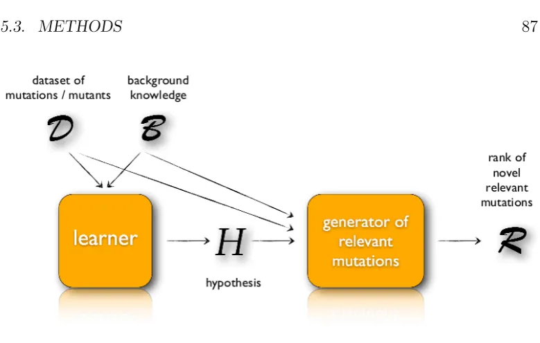
5.3.2 Algorithm overview . . . 87
5.3.3 Learning from mutations . . . 90
5.3.4 Learning from mutants . . . 92
5.4 Discussion and Future Work . . . 94
List of Tables
3.1 List of predicates used in the MLN Refiner. . . 38
3.2 Knowledge Base used in the MLN refiner. . . 39
3.3 Results for True Sub. Loc. . . 47
3.4 Results for Predicted Sub. Loc. . . 49
3.5 Results for True Sub. Loc. with Proxy. . . 50
3.6 Results for Predicted Sub. Loc. with Proxy. . . 51
4.1 List of SBR predicates. . . 64
4.2 List of SBR rules. . . 65
4.3 Area under the ROC curve values attained by Yip et al. [10], SBR, and SBR-∃n(SBR equipped with then-existential quan-tifier). . . 72
5.1 List of the ten most frequent rules learned on Dataset 1, sorted by average number of models they appear in. . . 92
5.2 List of the ten most frequent learned rules for Dataset 2, sorted by number of models they appear in. The table also includes the clause position(C,X), which is present in all models for different values ofX. . . 94
List of Figures
3.1 Diagram of the refinement pipeline. . . 38
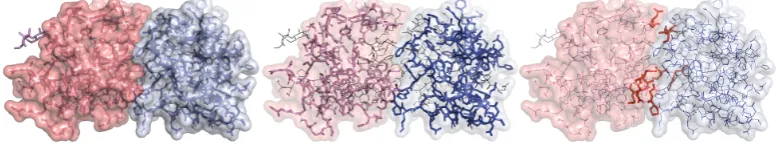
4.1 Two bound proteins and their interacting domains and residues, captured in PDB complex 4IOP. The proteins are a Killer cell lectin-like receptor (in violet) and its partner, a C-type lectin domain protein (in blue). Left: interaction as visible from the contact surface. Center: the two C-type lectin domains instan-tiating the interaction. Right: effectively interacting residues in red. . . 58
4.2 Visualization of the proposed method applied to a pair of pro-teins p and p0 and their parts. Circles represent proteins, domains and residues. Dotted lines indicate a parent-child relationship between objects, representing the parentpd and parentdr predicates. Solid lines link pairs of bound objects, i.e. objects for which theboundp,bounddorboundrpredicates are true. . . 61
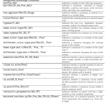
5.1 Summary of the background knowledge facts and rules. Mu-tID is a mutation or a mutant identifier depending on the type of the learning problem. . . 84
5.2 Mutation generation algorithm. . . 86
5.3 Schema of the mutation engineering algorithm. . . 87
5.4 An example of hypothesis, learned by Aleph on Dataset 1, for the NNRTI task with highlighted amino acid positions d by the hypothesis clauses. . . 88
5.5 An example of hypothesis, learned by kFOIL on Dataset 2, for the NNRTI task with highlighted amino acid positions covered by the hypothesis clauses. . . 89
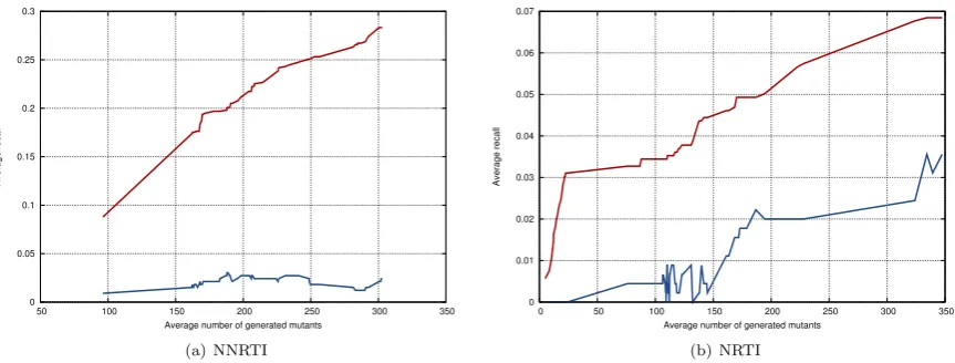
5.6 Mean recall of the generated mutations on the resistance test set mutations from Dataset 1 by varying the number of satis-fied clauses. The mean recall values in orange refer to the pro-posed generative algorithm. The mean recall values in green refer to a random generator of mutations. . . 91 5.7 Mean recall of the generated mutations on the resistance test
Acknowledgments
First of all, I would like to express my gratitude towards my supervisor, Andrea Passerini, for passionately teaching me the many unwritten rules of scientific research, which far too often go unnoticed to obtuse slackers like me. As I came to understand with time, research is a difficult craft, and problem solving can be a frustrating and utterly unrewarding activity. But thanks to Andrea’s continuous support, I somehow managed to get over the difficult times, and had the opportunity to enjoy the state of grace that only real numbers in the range [0,1], written in obscure monochromatic LATEX
tables, can give. Other than that, I would like to thank Andrea deeply and sincerely for being so friendly and generous, despite my embarrassing faults. I’d also like to thank two paradigmatic figures that I had the chance to meet here in Trento, Jacopo Staiano and Gabriele Catania. They managed to single handedly [sic.] transform the incongruous, desolate, fat misplaced lump of contemporary anti-seismic insanity that is our faculty, into an enjoy-able workplace. You are like metal water tanks in the middle of the desert: your faucets may be rusty, but inside you are full of wet. What does it mean? I do not know. But I think I got it right.
Then I’d like to thank Duy Tin Truong and Umut Avci, my office mates, for being delightful persons to work with, and for the time spent side-to-side crunching datasets, running experiments, and often sharing the same excited/derailed state of mind that positive/negative results cast upon us.
I’d like to extend my gratitude to Elisa Cilia, at the Universit´e Libre de Bruxelles; to the colleagues at the University of Siena: Claudio Sacc`a, Salvatore Frandina, and Michelangelo Diligenti; and to Bruno Lepri at the Fondazione Bruno Kessler, for the insightful discussions and support.
I’d also like to thank the Rost Lab at the Technische Universit¨at M¨unchen, and Gianluca Pollastri at the UCD School of Computer Science and Infor-matics, for making their software available.
Then there are all my friends, here in Trento and back at my hometown, too many to list here, who directly and indirectly supported my endeav-ors in scientific research, and provided many occasions for long sessions of
indiscriminate feasting and guzzling. Thank you.
Finally, my most sincere thanks go to my girlfriend Silvia, and to my parents Anna and Antonio, whose patience, reliability and constant support never cease to amaze and flatter me, and who have put so much effort into teaching me how to be a better person — even though I failed, far too often, to pay attention. It is to them that I wish to dedicate this thesis.
Chapter 1
Introduction
1.1
Motivation
The marriage between molecular biology and computer science is a long and fruitful one. Biologists have embraced computer science since the very be-ginning of the computer era in order to store the results of biological exper-iments, analyze the corresponding databases, find regularities, test hypothe-ses, and perform predictions. Due to the particularly complex and fuzzy nature of biological annotations, machine learning in particular has played an important role in biological research, providing many indispensable tools for forecasting properties of genes, proteins, RNA fragments, and other en-tities of biological interest. Thanks to their wide applicability and general success, predictive models have proved to be a valid support to wet exper-iments, leading to the development of hundred of computational prediction methods for a variety of protein, DNA and RNA properties, and a florid research field [11, 12].
Thanks to recent advancements in experimental methods, biological infor-mation has kept increasing in size and complexity. The rapid accumulation of huge amounts of data on many aspects of cell life has ushered many new, important questions. In general, the subject of molecular biology has broad-ened from the study of individual genes and proteins to a more integrated view: in the post-genomic era, open problems involve networks of interacting entities and their evolution, and can only be successfully answered by tak-ing into consideration the correlations linktak-ing the various types of biological objects.
Unfortunately, the classical tools provided by classical statistical or logical machine learning methods, such as Hidden Markov Models [13] and Support Vector Machines [14], are not ideally suited to deal with these problems,
which are, at once, intimatelyrelationalandstatistical. Purely logical models, such as those developed by the sub-field of Inductive Logic Programming [8, 15], do not provide a sound mechanism to handle noisy or incomplete data, and therefore have issues with biological data. On the other hand, Statistical Learning methods [16, 17, 18, 19], while designed to very naturally deal with noise and probabilities, can not be trivially adapted to handle relational data (in a sound manner): most of these methods are based on the assumption that examples are independently and identically distributed, which is violated by relational data. In other words, these two classes of learning methods offer complementary advantages, and are afflicted by complementary faults. As a result, neither of them is entirely appropriate for the new requirements imposed by complex biological prediction tasks.
Prompted by these difficulties, and similar ones arising in other research fields (e.g. network sociology and computational neuroscience), machine learners have developed novel methods, grouped under the umbrella term of Statistical Relational Learning (SRL) [1, 2], which generalize the classical models and merge the respective advantages. SRL methods are explicitly designed to perform predictions of complex objects, such as trees, graphs, multi-graphs and relational databases, and can natively take advantage of the correlations existing between the individual object parts.
Methods in SRL are typically based on some general, expressive, formal language, such as First-Order Logic (or subsets thereof), to encode both the data and a set of relations or constraints. The constraints offer the possi-bility of including additional human-readable background knowledge within the learning task, in order to restrict the model search space according to the instructions of domain experts, with potential gains in predictive accu-racy and learnability (especially in cases where data is scarce). Contrary to purely logical methods, where the constraints are deterministic, constraints in SRL can also be soft, in order to account for errors in the data or in the constraints. Inference and parameter learning are implemented as logical-probabilistic reasoning over the formal language, and enable sound handling of noise and missing data. Notably, the ability to include prior knowledge in the learning problem goes hand in hand with the formalization effort that is currently pervading biology and medicine, embodied by the development of formal ontologies, which are being applied to a growing number of biological databases [20, 21].
problems. In the next few sections we present a high-level overview of the problems tackled in the next chapters.
1.1.1
Protein Feature Predictor Refinement with Markov
Logic
Computational methods for the prediction of protein features from sequence are a long-standing focus of bioinformatics. A key observation is that several protein features are closely inter-related, that is, they are conditioned on each other. Researchers invested a lot of effort into designing predictors that exploit this fact. Most existing methods leverage inter-feature constraints by including known (or predicted) correlated features asinputsto the predictor, thus conditioning the result.
By including correlated features as inputs, existing methods only rely on one side of the relation: the output feature is conditioned on the input fea-tures. In Chapter 3 we show how to jointly improve the outputs of multiple correlated predictors by means of a probabilistic-logical consistency layer. The logical layer enforces a set of weighted first-order rules encoding biologi-cal constraints between the features, and improves the raw predictions so that they least violate the constraints. In particular, we show how to integrate three stand-alone predictors of correlated features: subcellular localization (Loctree[4]), disulfide bonding state (Disulfind[5]), and metal bonding state (MetalDetector[6]), in a way that takes into account the respective strengths and weaknesses, and does not require any change to the predictors them-selves. We compare our methodology against two alternative refinement pipelines based on state-of-the-art sequential prediction methods.
1.1.2
Multi-level Protein–Protein Interaction Prediction
Protein–protein interactions can be seen as a hierarchical process occurring at three related levels: proteins bind by means of specificdomains, which in turn form interfaces through patches of residues. Detailed knowledge about which domains and residues are involved in a given interaction has extensive applications to biology, including better understanding of the binding process and more efficient drug/enzyme design. Alas, most current interaction pre-diction methods do not identify which parts of a protein actually instantiate an interaction. Furthermore, they also fail to leverage the hierarchical nature of the problem, ignoring otherwise useful information available at the lower levels; when they do, they do not generate predictions that are guaranteed to be consistent between levels.
In Chapter 4 we formalize the problem as a multi-level learning task, with one task per level (proteins, domains and residues), and propose a machine learning method that collectively infers the binding state of all object pairs. Our method is based on Semantic Based Regularization (SBR), a flexible and theoretically sound machine learning framework that uses First Order Logic constraints to tie the learning tasks together. We introduce a set of biologically motivated rules that enforce consistent predictions between the hierarchy levels.
We study the empirical performance of our method using a standard validation procedure, and compare its performance against the only other existing multi-level prediction technique. We present results showing that our method substantially outperforms the competitor in several experimental settings, indicating that exploiting the hierarchical nature of the problem can lead to better predictions. In addition, our method is also guaranteed to produce interactions that are consistent with respect to the protein–domain– residue hierarchy.
1.1.3
Forecasting Viral Mutants
Viruses are typically characterized by high mutation rates, which allow them to quickly develop drug-resistant mutations. Mining relevant rules from mu-tation data can be extremely useful to understand the virus adapmu-tation mech-anism and to design drugs that effectively counter potentially resistant mu-tants.
the drug. The algorithm learns a set of relational rules characterizing drug-resistance and uses them to generate a set of potentially resistant mutants. Learning a weighted combination of rules allows to attach generated mutants with a resistance score as predicted by the statistical relational model and select only the highest scoring ones.
Promising results were obtained in generating resistant mutations for both nucleoside and non-nucleoside HIV reverse transcriptase inhibitors. The ap-proach can be generalized quite easily to learning mutants characterized by more complex rules correlating multiple mutations.
1.1.4
Publications
The three chapters are taken from the following papers:
• Stefano Teso, Andrea Passerini – “Joint Probabilistic-Logical Refine-ment of Multiple Protein Feature Predictors”, BMC Bioinformatics (in press).
• Claudio Sacc`a, Stefano Teso, Michelangelo Diligenti, Andrea Passerini – “Improved Multi-level Protein–Protein Interaction Prediction with Semantic-based Regularization”, BMC Bioinformatics (submitted). • Elisa Cilia, Stefano Teso, Sergio Ammendola, Tom Lenaerts, Andrea
Chapter 2
Background
2.1
Molecular Biology of Proteins
This thesis is concerned mostly with problems related to proteins. Proteins are polypeptides, biological molecules of variable size, often composed of mul-tiple parts orchains, which carry out many different functions within the cell, including (but not limited to) metabolism, DNA transcription, translation and synthesis, regulation of gene expression, signal transduction (in response to external stimuli or internal events), and antigenic response. Most of the activities that take place within the cell are enacted by proteins [24, 25], in-cluding those involved in the mechanisms of inherited and infectious diseases. Complete details on the composition, properties and concerted behavior of proteins within the organism (theproteome), are a key factor in elucidating the genotype-phenotype relationship, with all the scientific and medical con-sequences it entails. This observation motivates much of the research done in bioinformatics topredictsuch information, which are generally difficult or expensive to annotate experimentally, from the available data.
In this section we give a short exposition of the molecular biology of proteins, tailored towards the scope of this thesis. We describe the three basic properties of proteins (sequence, structure, and function) and the relation between them; we give details about the means by which proteins interact, and why; and sketch how proteins evolve by natural selection. Of course, our exposition only scratches the surface of protein biology. For a broader and deeper treatment of the subject, we refer the reader to the many excellent textbooks available [24, 25, 26].
2.1.1
Sequence
A protein can be described in terms of its chemical composition. Each pro-tein is uniquely identified, modulo neutral mutations, by a specific sequence of twenty canonical amino acids, small organic molecules that have a com-mon chemical component (an amine and a carboxylic acid functional group) and a variable component, theside chain. The common part forms the back-bone of the protein, while the side chain determines the identity, chemical properties, and size of each amino acid within the protein sequence. From a computational point of view, a protein sequence can be thus described as a string of arbitrary length on an alphabet of twenty symbols — with one character for each amino acid.
molecular mechanism that operate on them. Given the genetic sequence, it is possible to derive the corresponding protein sequence by mapping triplets of nucleotides into amino acids — the mapping between the two alphabets is the celebrated genetic code. Since whole-genome sequencing is both afford-able and very efficient, sequence information currently represents the most abundant form of information on proteins.
The correspondence between genes and proteins, however, is not bijec-tive, due to two mechanisms: alternative splicing andhomology. Alternative splicing is the process by which, during transcription, different sets of exons (coding regions) of a gene are shuffled and adjoined, allowing the gene to encode for multiple proteins. On the other hand, a genome may hold mul-tiple copies of the same gene, i.e. paralogues, which encode for the same set of proteins. Despite these issues, there exist rather advanced techniques that — by aligning a newly sequenced genome to already annotated ones — allow to determine the majority of the genes (and therefore proteins) in an organism [27].
A basic assumption in biology is that the sequence, orprimary structure, of a protein completely determines its three-dimensional (tertiary) struc-ture [28], which in turn is responsible for the biological function expressed by the protein itself [29]. While the relationship is thought to be (roughly) deterministic, the exact mechanisms by which the sequence — known for the majority of proteins — maps to the structure and function of the protein itself, are still largely unknown. This state of affairs motivates much of the research done on protein function prediction in computational biology [11].
2.1.2
Structure and Structural Properties
The mismatch between our knowledge of sequence and structure can be at least partially retraced to the technological gap between current experimen-tal methods for sequencing and structure determination. Methods in the latter category, such as nuclear magnetic resonance spectroscopy [30], X-ray crystallography [31], and electron microscopy [32] are not high-throughput, requiring time consuming sample preparation, and are not always applica-ble (e.g. X-ray crystallography requires the protein to be first crystallize, which is not always feasible). As a result, the number of resolved structures accounts for only a fraction of the sequenced proteins [33].
composition of the protein sequence [36]. Since the major driving forces are physico-chemical in nature (namely the hydrophobic effect, the formation of hydrogen bonds and electrostatic interactions, and the conformational en-tropy due to restricted degrees-of-freedom of the chain [37]), folding takes place autonomously under suitable conditions. The formation of secondary structure elements [38] and post-translational modifications [39] (such as the addition of disulphide bonds [40] and acetyl functional groups [41]) also play a role in guiding and stabilizing the folding process. Correctly folded struc-tures are thought to fluctuate around theglobal minimum of the free-energy function. In order for proteins to successfully reach said global minimum, the energy landscape is thought [36] to be shaped like a rough funnel, although the exact mechanisms are not yet clear. Folding plays a crucial role in bi-ology: since structure determines function, mis-folded protein may express impaired, null or toxical activity [42]. As a matter of fact, there are many in-herited diseases which have been attributed to mutation-induced misfolding, e.g. Alzheimer’s and Parkinson’s diseases, cystic fibrosis and some neurode-generative diseases [42, 34].
Several factors contribute to the complexity of the folding problem. An important component are the non-local contacts, i.e. long-range correlations between residues, which constrain and stabilize the folding process [43]; these correlations also render computational simulations of folding very compu-tationally demanding. It is also difficult to experimentally determine the folding intermediates sampled during the process and the alternative final conformations [44]. Furthermore, some proteins are only stabilized by exter-nal factors such as post-translatioexter-nal modifications [39], which are hard to capture computationally. Despite the advancements in computer simulations and machine learning methods for structure predictions, these still have lim-ited applicability [45], hindering our ability to automatically determine the structure of newly sequenced proteins.
The tertiary structure of proteins lodges many types of well-defined local structures which have critical biological roles, and can, notably, be inferred independently. These characteristic sub-structures include secondary struc-ture elements, catalytic sites, binding sites, and disordered regions. Knowl-edge about their displacement can be leveraged to reconstruct the global structure of the protein, and define its function; this observation stands at the heart of many hierarchical structure and function prediction methods.
its strong structural and functional role, the core is the most evolutionarily conserved region of the protein: mutations that alter the volume of the core often have a negative impact on protein stability [42].
The secondary structure (SS) of a protein consists of very recognizable fragments of well defined, stable, and conserved three-dimensional residue arrangements, the SS elements. The two most frequent configurations are α-helices and β-sheets [25], which are ubiquitous in protein space. The full list of secondary structure types is listed in the Dictionary of Protein Sec-ondary Structures (DSSP) [38], which classifies proteins according to their secondary structure composition. Contrary to tertiary structure, which is a global property of the protein sequence, secondary structures are the result of local contributions of hydrogen bonds between nearby residues [46], and as such are thought to act as building blocks for intermediates during fold-ing. Secondary structure elements are tailored towards specific functions. For instance,α-helices are commonly found in transmembrane proteins [47], which attach to the lipid bilayer of the cell wall, and are pivotal for enabling transmembrane proteins to participate to signaling and cell-cell recognition. Catalytic sites play a central role in enzymes [48], i.e. proteins that alyze chemical reactions. Thanks to their physico-chemical properties, cat-alytic sites can recognize and capture the substrates of a reaction, and care-fully position them in order to facilitate (i.e. lower the activation energy of) the reaction. Only a fraction of the residues accessible within the ac-tive sites participate in the reaction; the remaining residues may be inert, or only help in capturing the substrate. Upon binding, substrates may induce a conformational change, which may expose other active sites in the protein, or detach other substrates [49]. In general, catalytic residues owe their ef-ficacy to both their chemical composition and spatial arrangement, and are typically highly conserved. Identification of catalytic sites is fundamental for identifying enzymes and characterizing their function. A complete hand curated list of annotated catalytic sites can be found in the Catalytic Site Atlas (CSA) database [48].
contact surface or clogging the hot spots, i.e. those residues that contribute the majority of the binding energy [53].
Finally, we end this section with a note on protein flexibility. Protein structures have long been known to be dynamic, as molecular shape vari-ations occur naturally as a consequence of thermal fluctuvari-ations [54]. More importantly, many protein — e.g. enzymes —relyon their structure to switch between alternate conformations, which have different functional roles. For instance, depending on its current state, a protein may expose different func-tional regions. However, it has been recently observed that a large fraction of eukaryotic proteins (over 30% [55]) present structural segments that are inherently disordered, i.e. segments with no definite secondary or tertiary structure. Even though their exact role is still unclear [56], inherently disor-dered proteins have been observed to play a role in intracellular signaling and regulatory processes [55], and are known to have strong molecular recognition capabilities [57], enabled by their ability to undergo structural stabilization upon binding [58]. Disordered proteins have been associated with several pathological conditions, such as cancer and cardiovascular diseases [59, 60].
2.1.3
Function
Protein function is a compound term to refer to the overall behavior of a protein and its role within the proteome. Being so diverse, protein function has been defined in different, often conflicting terms over time. Recently, however, there has been growing consensus on formalizing protein function according to the Gene Onotology (GO) [20], a wide vocabulary of shared, controlled terms. GO terms are organized in a hierarchy according to a general-to-specific relation: terms in the GO form atree, where parent terms are strictly more general than their children [20].
The GO includes keywords for three orthogonal aspects of protein func-tion: i) what molecular function is displayed by the protein (e.g. enzymatic reaction), ii) what biological processesit participates in (e.g. cell cycle, gene regulation, apoptosis), and iii) what cellular components it resides within (e.g. nucleus, cytosol, mitochondrion, etc.).
2.1.4
Interactions
Proteins do not act in isolation. In order to carry out their function, most proteins interact with (bind to) other proteins. A group of proteins and their interactions is called a protein–protein interaction network (PIN). PINs cap-ture a static, protein-level snapshot of the overall topology of protein inter-actions. The totality of interactions expressed by a proteome is called the interactome. Physical interactions are the workhorse of cell life and develop-ment [64], and play an extremely important role both in the mechanisms of disease [65] and in the design of new drugs [66].
Physical interactions between proteins can be seen at different levels of detail. At the highest level, proteins interact to perform some joint func-tion [67], which is effectively mediated by the interacfunc-tion itself [68]. The propagation of function at the network-level forms the basis of biological pathways, evolutionarily conserved sub-modules of the PIN that are spe-cialized for a particular function. Pathways can be distinguished in three varieties (metabolic pathways, regulation pathways, and signal transduction pathways), as accurately annotated in the KEGG encyclopedia [69]. In par-ticular, signal transduction pathways consist of groups of interacting proteins that collectively transport information about events in the cell, e.g. apoptosis (programmed cell death).
At a lower level, the same interaction occurs between a pair of specific domains appearing in the proteins. Domains are conserved sub-regions of protein sequence/structure that perform a specific function, e.g. partner recognition, catalysis, etc. The types of the domains involved in an interac-tion characterize the funcinterac-tional semantics of the latter [70].
At the lowest level, the interaction is instantiated by the binding of a pair of protein interfaces, i.e. patches of solvent accessible residues with compatible shapes and chemical properties [71]. The low-level features of binding sites determine whether the interaction is transient or permanent, whether two proteins compete for interaction with a third one, etc.
de-sign [66], metabolic reconstruction and engineering [77], and identification of hot-spots [78] in the absence of structure information.
Notwithstanding the increased availability of interaction data, the nat-ural question of whether two arbitrary proteins interact, and why, is still open. The growing literature on protein interaction prediction [79, 80, 81] is symptomatic of the gap separating the amount of available data and the effective size of the interaction network [82]. Furthermore, protein–protein interaction data is under-characterized at the domain and residue levels: the current databases are relatively lacking when compared to the magnitude of the existing body of data about protein-level interactions [76]. At the time of writing, the PDB hosts 84,418 structures, but merely 4,210 resolved com-plexes1. The latter cover only a tiny fraction of the interactions stored in
databases such as BioGRID [83] and MIPS [84].
2.1.5
Evolution
During the normal life cycle of the cell, DNA may be affected by mutations, i.e. the addition, removal or substitution of some of its bases [85]. Mutations have multiple causes, including naturally occurring errors in DNA replica-tion, mutagens (chemicals, radiareplica-tion, etc.), and pathogens. In an individual mutation event, the number of mutated bases is typically low. In particu-lar, single nucleotide polymorphisms (SNP) comprise the majority of known mutations [86].
Due to the redundancy of the genetic code a mutation may change a nucleotide triplet into a new triplet that encodes the same amino acid. Even though the accumulation of such events, calledsynonymousmutations, is thought to play a significant role in evolution [87], individual synony-mous mutations have no immediate effect at the protein level. Conversely, non-synonymous mutations can induce different effects, including acquisi-tion and loss of funcacquisi-tion. Mutant proteins may exhibit changes in physical and chemical properties, folding and stability, activity, structure and func-tion [42, 88, 89, 90]. A single mutafunc-tion affecting a catalytic site may for instance alter the efficiency of the enzyme. At the network level, mutations may disrupt the affinity with binding partners or form novel binding sites, which in turn influence the interaction network topology and biological path-ways the proteins participates into.
In general, mutations occurring in functional regions of a protein are likely to have a deeper impact, and are thus subject to more stringent
con-1According to http://www.rcsb.org/pdb/statistics/holdings.do, retrieved
straints [91]. Mutations affecting protein stability or folding (which may therefore have immediate detrimental effects on the host), are more likely to be rapidly removed from the genetic pool by natural selection. It is known that many serious inherited diseases, e.g. cancer and some neuromuscular pathologies, are due to mutations [92], and in particular to nsSNPs [93].
2.2
Machine Learning
Machine learning is a large research field and covers a broad range of method-ologies and problems, catering techniques from a number of other disciplines, including (but not limited to) mathematical optimization, statistics, formal languages, and artificial intelligence. In this section we focus on three areas of machine learning, namelyprobabilistic graphical models,kernel methods, and inductive logic programming, and further provide a short introduction to Sta-tistical Relational Learning, which form the basis for the methods described and used in the next chapters.
In the following we will focus on supervised learning, where the goal is to find a mappingbetween inputs and outputs that generalizes over unseen inputs. While learning in a mathematical sense has a broadly accepted foun-dation, the exact meaning of “generalization”, as well as the performance measures used to quantify the generalization ability of a learning machine, depend on the particular learning framework under examination. We will briefly discuss these details shortly, and refer the reader to any of the several exhaustive books on the subject [19, 18, 16, 17] for a more detailed treatment. The other major machine learning flavor of machine learning is unsuper-vised learning [97], where the goal is to find “interesting” patterns — e.g. clusters, sub-spaces, latent representations — in the data. We will not make use of unsupervised learning techniques in this thesis. We will also ignore other flavors of learning, such asreinforcement learning [98], and postpone a description of semi-supervised/transductive learning [99] to a later Chapter.
2.2.1
Statistical Learning
Statistical learning is a sub-field of machine learning that borrows tools from statistics and decision theory to i) formally define the semantics of learning in a mathematical sense, and ii) solve the resulting numerical problems. Both kernel machines and probabilistic graphical models are part of statistical learning.
Insupervisedstatistical learning, the learning algorithm is given a training set of input-output pairs D :={(xi, yi)}ni=1, with inputs x∈ X and outputs
y ∈ Y, where the pairs are drawn i.i.d. (independently and identically dis-tributed) from a fixed but unknownjoint distribution:
(xi, yi)∼pX,Y(X, Y)
but (again) unknown distributions:
x∼pX y|x∼pY|X
whose product is the joint2. Here we do not impose any restrictions on
the form of the input and output domains X and Y. In classical learning scenarios, the input domain X is a real-valued vector field Rd (for some d≥1), called the feature space, andY is either the set of binary class labels Y = {0,1}, in which case learning is a classification problem, or a real-valued vector field Y =Rd0 (for some d0 ≥1), in which case we talk about a regression problem.
As already hinted to, learning amounts to finding a (predictive) function (also called model or hypothesis) f : X → Y, taken from a set of possible models F, that is able to generalize to unobserved samples: learning is in-ductive, as it aims to discover a general model of the data from a finite set of examples. A model f on a dataset D has good generalization ability if its output is “close enough” to the real output for all possible inputs. The notion of “closeness” can be formalized as a loss function.
Definition 2.2.1 (Loss function) A function ` : Y × Y → R is a loss function if (i) `(y, y0)≥0 for ally, y0 ∈ Y, and (ii) `(y, y) = 0 for all y∈ Y. The quantity`(y, y0) measures the penalty or cost incurred when a model predicts y0 while the correct output is y. Here, (ii) ensures that there is no penalty when the predicted output is correct. A loss function implicitly defines the risk of a learning machine f, which measures the total error f entails when applied to the full domainX × Y, i.e. its generalization ability: Definition 2.2.2 (Risk) Given a loss function `, the risk (or total error) incurred by a model f is:
R[f] :=EpX,Y[`(Y, f(X)] =
Z
X ×Y
`(y, f(x))pX,Y(x, y)d(x, y)
The choice of loss function is problem dependant. Classical loss functions for classification, assuming that the possible classes are y = 1 and y = −1, are [100] the zero-one loss function `(y, y0) := I[y = y0], the square loss `(y, y0) := (1−yy0)2, and the hinge loss `(y, y0) := max(0,1−y ·y0).
Loss functions for regression include the square loss `(y, y0) := (y0 −y)2, the
absolute value loss `(y, y0) := |y−y0|, and the -insensitive loss `(y, y0) := max(|y0−y| −,0).
By seeking the modelf with maximum generalization ability — or equiv-alently minimum risk — we obtain the so-called risk minimization criterion.
Definition 2.2.3 (Risk minimization) Given a dataset D and a set of candidate models F, find the model f∗ ∈ F that minimizes the risk:
f∗ := arg min
f∈FR[f]
The issue is that, of course, the joint pX,Y is unobserved: all the learning method is allowed to learn from is the datasetD, which (likely) captures only a very small portion of all possible combinations of inputs and outputs. This limitation implies that we can not compute the risk functional. Instead, we can resort to estimating an approximation thereof, the empirical risk, based on the empirical joint ˆpX,Y. This reasoning leads to theempirical risk minimizationprocedure.
Definition 2.2.4 (Empirical risk minimization) Given a loss function `, the empirical risk incurred by a model f over a dataset D ={(xi, yi)}ni=1
is:
ˆ
R[f] :=EpˆX,Y[`(y, f(x))] =
1 n
n
X
i=1
`(yi, f(xi))
Empirical risk minimization amounts to fininding the model f ∈ F that has minimizes the empirical risk:
f∗ := arg min
f∈F
ˆ R[f]
Despite its many forms, empirical risk minimization (ERM) stands at the heart of many machine learning methods. There are other optimality criteria used in the literature, such asmaximum likelihoodfor probabilistic graphical models (which we sketch in Section 2.2.3), which states that the best model is the one most likely to have generated the data (modulo Bayesian priors), and maximum entropy, which postulates that the best model is the one that has maximal uncertainty given the observations [101]. All of these criteria, ERM included, boil down to mathematical optimization over the set of candidate functions — and the efficacy of the search algorithm depends crucially on the structure ofF and on the choice of loss function. For the purpose of this section, for simplicity we will focus on the ERM formulation of learning.
training set ˆpX,Y is not a faithful sample for the joint pX,Y as a consequence of noise or missing data. In such conditions, the model mayoverfit the data. To lessen the chances of overfitting, it is useful to restrict the set of candidate models F, e.g. by penalizing complex hypotheses. This involves including a regularization term (orprior) over F. How to do so depends on the method at hand, but the two most common regulariers are the `2 loss,
which can be seen as a Gaussian prior over the model complexity, and the`1
loss, that corresponds to a Laplacian prior and favors more sparse models. Notwithstanding these commonalities — namely, learning as optimiza-tion, use of regularizers/priors, reliance on i.i.d. assumptions for the data, and requiring data to be formatted in a propositional, or attribute-value, rep-resentation —, statistical learning methods vary greatly, and each method offers its particular set of trade-offs. We will omit a detailed treatment of the details, which is far beyond the scope of this work.
Model Selection
In order to perform model selection, i.e. picking a learned model out of many, it is necessary to estimate its generalization ability by evaluating its empirical performance on an independent dataset, called the test set. The test set must be drawn from the same distribution p(X, Y) as the training set, but must also be as statistically independent from the latter, as to avoid optimistically inflating the model performance. There are a few alternative procedures to select the test set [16, 17].
The most widely used procedure is cross-validation (CV). In CV, the dataset is partitioned into k folds, with k = 10 in typical scenarios. The procedure consists of k rounds: in each iteration, a model is learned from of k −1 folds and tested on the remaining one. The overall performance is estimated as the average performance over all rounds. Notably, cross-validation makes use ofallthe data available for training. Two variants on the theme are leave-one-out, where there are exactly as many folds as there are data instances, andstratifiedcross-validation, where the proportion of classes is kept fixed between folds — this is particularly important in cases of class unbalance. It has been shown that cross-validation with moderate choices of k reduces the variance and increase the bias [102], and that stratification produces more accurate results.
Finally, the holdout procedure consists of splitting the dataset into two mutually exclusive subsets. The bigger one, typically accounting for 2/3 of the data, is used for training, while the rest (the holdout) is used for testing only. The holdout is a pessimistic estimator [102], whose performance depends crucially on the selection of the test set. Moreover, since it does not prescribe repeated trials, the holdout method makes inefficient use of the data. Because of these issues, and since the cross-validation provides (under mild conditions [103]) better accuracy, the holdout has been largely superseded by cross-validation.
2.2.2
Kernel Methods
Kernel methods [104, 105, 106, 107] are one of the most popular classes of methods in machine learning, due to their efficiency, versatility, and theoret-ical soundness. Support Vector Machines, in particular, have been applied almost universally in the field of computational biology (see e.g. [12]), also thanks to the availability of excellent implementations [108, 109, 110]. Ker-nel methods come in a multitude of forms, and over time have been adapted to perform a variety of learning tasks.
The original Support Vector Machine (SVM) classifier, which laid the groundwork for the whole field, has been published in Vapnik et al. [111] and in Cortes and Vapnik in [14]. Given a dataset of attribute-value inputs xi ∈ Rd with binary class labels yi ∈ {−1,1}, the SVM attempts to find a separating hyperplane (or weight vector) w ∈ Rd, with offset b ∈
R from the origin, that maximizes themargin (hence the termmax-margin) between instances belonging to the two classes. Given w and b, predicting the class of a novel input x amounts to checking on which side of the hyperplane it resides, i.e. the sign of hyperplane equation:
f(x;w, b) :=σ(wTx+b)
where σ(t) = 1 if t ≥ 0, and −1 otherwise. One of the most important aspects of SVM max-margin training is that it guarantees that the true error of the learning machine is probabilistically bounded by the training set error (empirical risk) [112]. This result is one of the key advantages of Support Vector Machines over more heuristic methods.
The primal form of the training procedure [111] for linearly separable classes, where a separation hyperplane always exists, is:
arg min
w,b 1 2kwk
2
By minimizing the modulo kwk of the weight vector, SVMs maximize the separation between the classes. In the non-separable case, the softSVM for-mulation [14] introduces additional slack variablesξi to account for examples that necessarily violate the separation assumption. The primal form of soft SVM can be written as:
arg min
w,b,ξ 1 2kwk
2+C
n
X
i=1
ξi
s.t. yi(wTxi−b)≥1−ξi, ξi ≥0, i= 1, . . . , n
Here C is a hyper-parameter that balances the model complexity and the training set error, and can be used to control overfitting. When written in this form, it is clear that the term kwk2 acts as a regularizer, and behaves
analogously to a Gaussian prior.
The optimization problem in the primal is a quadratic program, which can be solved by the Lagrange multiplier method. The Lagrangian dual form of (soft) SVM is:
arg min n
X
i=0
αi− 1 2
X
i,j
αiαjyiyjxTi xj
s.t. 0≤αi ≤C, i= 1, . . . , n; n
X
i=1
αiyi = 0
where the αi are per-instance variables introduced by the dual transforma-tion. The instances for which αi >0 are called the support vectors, and are typically less than n. The hyperplane w can be reconstructed from the set of support vectors by means of the linear combination w =P
iαiyixi. The fact that the max-margin hyperplane only relies on a subset of the instances, namely on the support vectors, renders SVMs more robust to noise.
Most importantly, since the data appears in the dual problem only in the form of dot products — i.e., xiTxj —, it is possible to substitute to the canonical dot product of Euclidean space any other dot product. This is the so-called “kernel trick” [105]. For an arbitrary input domainX, a kernel is a function k:X × X →R≥0 that satisfies an additional condition.
Definition 2.2.5 (Kernels [113]) Given a function k as described above, and a set of objects {xi}ni=1 the Gram matrix K ∈Rn
×n is defined as: Kij :=k(xi, xj)
If the Gram matrix of k is positive semi-definite, i.e. if it satisfies the con-dition:
X
i,j
for all vectors c, then k is a kernel.
Kernel functions are important because they always represent a dot product in some Reproducing Kernel Hilbert Space (RKHS) [113]. Therefore, kernel functions can be used in place of regular dot product in SVMs. Furthermore, the Representer Theorem [113] guarantees that, whenever the function k is a kernel, SVM training is convex, and its optimum — the max-margin hyperplane — can be expressed as a kernel expansion of the form:
f(x) = n
X
i=1
αiK(x, xi)
Representer theorems have been devised for a multitude of kernel methods, and stand at the basis of the many efficient algorithms for SVMs, including Sequential Minimal Optimization [114] and the Cutting Plane algorithm [115] Alternative kernels allow to perform classification with arbitrary objects, including structured and relational ones. The literature flourishes with ker-nels for different data types. The most basic kerker-nels include the polynomial kernel and radial basis functions [113], which allow to include correlations between instances into the learning problem. Kernels for structured data also exist, for instance for attributed graphs (useful for representing chem-ical structures) and relational databases [116]. There are also more exotic kernels, like the Fisher kernel [117], which allows to define the similarity between structured objects in terms of a probabilistic graphical model (or stochastic grammar).
As we have seen, kernel methods have a number of advantages: they are efficient, since the training problem is convex, they can handle a plethora of different objects as inputs (even infinite dimensional ones) via the kernel trick, and they have a very firm theoretical basis. Support Vector Machines can be currently considered astock learning method, and have been used as a black box throughout the computational biology literature. Furthermore, the core idea of max-margin learning has developed into a wealth of kernel machines, including regression [118], one-class classification [119], multi-class classification [120], transductive learning [121], and structured output predic-tion [122, 123], among many others. Despite its limitapredic-tions, attribute-value representations allow kernel machines to easily integrate data from different sources — simply by concatenating the various features in a single feature vectorx, although there are more complex schemas, and, as always, caveats — a task often required in computational biology.
predictions. For binary classification, a practical method is the one proposed by Platt [124], who suggests to fit a sigmoid to the predicted margin, and estimate a probability by evaluating the sigmoid. Clearly, this method is heurisic, as the sigmoid is not a density function. Another issue of most kernel methods is that they can not handle relational outputs. This restric-tion has been recently lifted by structured output SVMs [122, 123], but still affects the majority of kernel methods. Other limitations include the inabil-ity to natively deal with missing data (requiring the use of heuristics like the Expectation Maximization algorithm or pre-processing, e.g. removing instances with missing features) [125] and unbalanced classes. Finally, con-trarily to logic-based methods, the learned SVM parameters are difficult to interpret, even for domain experts.
2.2.3
Probabilistic Graphical Models
Probabilistic graphical models (PGMs) are a principled and elegant frame-work to compactly represent high-dimensional joint distributions, which com-bines probability theory and graph theory [126, 127]. Joint distributions can represent arbitrary dependencies between variables, for instance between in-puts (i.e. observed variables) and outin-puts of a prediction problem, and thus offer excellent expressivity and flexibility. Alas, learning a full joint dis-tribution is infeasible: even in the simplest case, i.e. a multinomial over n binary variables, fitting is equivalent to learning 2nparameters from the data. The main insight of PGMs is that, by selectively inserting independencies in the full joint, we can limit the complexity of the model — i.e., the num-ber of parameters to be estimated —, drastically improving its learnability (especially when there is little data available), while retaining its expressive power. Contrarily to statistical learning methods like kernel machines, PGMs are designed to deal with relational data, and their predictions are natively accompanied by a confidence in the form of probabilities.
The basic idea is to define a joint by means of a graphG= (X, E), whose nodes are random variables, and whose local dependencies are captured by the topology of the graph. In particular, variables connected by an edge are conditioned on each other. The exact semantics then depends on whether the graph is directed or undirected, in which case we talk of Bayesian networks (BNs) and Markov networks (MNs), respectively. The two classes of models differ in what distributions they can represent [128]. While the two definitions are fully general, in the following we will restrict our attention to models with discrete random variables.
di-rected acyclic graph (DAG) G= (X, E), where X ={Xi}ni=1 is a set of
ran-dom variables and E ⊆ X ×X is a set of directed edges, encodes the joint probabilty distribution:
p(X) = n
Y
i=1
p(Xi |π(Xi))
where π(Xi)is the set of parents of node Xi. Here the functional form of the conditional distributions is assumed to be known beforehand.
Intuitively, a BN defines a set of causality relations in terms of local in-fluences between a node and its parents. For discrete random variables, the local conditional distributionsp(Xi |π(Xi)) are multinomials, parameterized by a conditional probability table (CPT), whose size is proportional to the number of parents and the number of their states. From a computational perspective, this cuts the number of parameters needed to specify a discrete joint distribution on n variables from O(mn) for a complete graph (for ran-dom variables taking values in {1, . . . , m} with n parents each) to a much smaller number that depends only on the graph topology.
Definition 2.2.7 (Markov network) A Markov network defined on an undi-rected graph G = (X, E), where X = {Xi}ni=1 is a set of random variables,
E ⊆X×X is a set of undirected edges, and C is the set of maximal cliques in G, encodes the joint probabilty distribution:
p(X) = 1 Z
Y
C∈C
ψC(XC) = 1 Z exp
X
C∈C
φC(XC)
HereXC is the subset of variablesX appearing in a cliqueC, theφC := logψC are arbitrary positive real-valued functions, calledclique potentialsorfactors, that evaluate the compatibility of the variables XC, and Z is a normalization term.
Rather than on causality, MNs rely on undirected correlations between the nodes. The clique potentials φC measure the “compatibility” between vari-ables in a clique, and higher values ofφC identify more likely configurations. The potentials need not be conditional distributions. The normalization term Z, also calledpartition function, converts the unnormalized exponential into a proper probability distribution.
It is worth mentioning that the majority of MNs used in the literature restrict the clique potentials to a linear form, and thus effectively encode a log-linear model:
p(X) = 1 Z exp
X
C∈C
Here the functionsfC = (fC1, . . . , fCd) act asfeature functions, and their con-tribution to the potential is modulated by a set of real-valued weights wC. Positive weights are associated to features that render the configuration more likely. A natural way to implement the feature function is as indicator func-tions, that evaluate to 1 if a particular property is satisfied by the configu-ration of XC, and to 0 otherwise. This very useful reinterpretation of clique potential has been introduced in the machine learning literature by Lafferty, McCallum and Pereira in [129].
While conceptually similar, BNs and MNs differ in what kinds of distri-butions they can represent [126]. In particular, BNs are more fit to model complex causal processes, and have been applied in computational biology to problems related to the prediction of bidimensional protein properties (such as secondary structure [130]), to gene regulation [131], and to collective pro-tein function prediction [132], among others. Particular instantiations of BNs include Markov Chains, Hidden Markov Models (HMMs) [13], and Dynamic Bayesian Networks (DBNs) [133]. On the other hand, MNs are more suited to problems with no definite directionality, e.g. spatial and relational data, where the correlations are symmetrical. These cases can not be easily cap-tured with BNs. MNs and their instantiations, such as Conditional Random Fields (CRFs) [129], have been applied to a wealth of problems, in particular in the areas of spatial statistics [134], computer vision [135], natural language processing [136], and many other tasks.
Inference in PGMs has different variants [137]. In general, given a set of observed nodes X =x, theevidence, the goal is to compute the most likely state y∗ of a set of unknown, query nodesY. This form of inference is called
maximum a-posteriori (MAP), and can be written as: y∗ = arg max
y p(y|x) (2.1)
Another type of inference involves computing the conditional probability of a given stateY =y given the observations X =x, and can be written as:
p(y |x) = p(x, y)
p(x) (2.2)
order to compute Equation 2.2:
p(y|x) =X w
p(y, w|x) = X w
p(y|x, w)p(w|x) (2.3)
This additional summation renders inference more computationally complex. Similarly to most other probabilistic models, given a set of m examples D, learning in graphical models amounts to maximize the likelihood of the modelf with respect to the dataD, that is, to compute arg maxp(f |D). As is often the case in machine learning, in order to avoid overfitting, the param-eters (i.e. CPTs for BNs and weights for log-linear models) are equipped with suitable priors. Restricting the discussion to log-linear Markov Networks, the maximum (log) likelihood equation can be written as:
arg max w m X i=1 1
Z exp −
X
C∈C
wTCfC(xiC)
!
where the xi
C are the observed values of variables in clique C for example i [137]. The log-likelihood, being a concave function of the weights [126], can be minimized efficiently by stock first-order and second-order continuous optimization methods.
Alas, evaluating the objective function during the optimization procedure is equivalent to performing inference in the model, which turns out to be, in the worst case, intractable [137]: although there are general algorithms to compute the conditional p(y | x) (e.g. message passing algorithms over the junction tree [126], which can be applied equally to directed and undirected graphical models), exact inference in PGMs is NP-complete [126]. In partic-ular, the complexity of inference depends on the treewidth of the model, i.e. the size of the largest clique in the junction tree. This fact makes inference tractable only for models with low treewidth. As already hinted to, exact weight learning, which employs inference as a subroutine, also learning is intractable.
inference in PGMs can also be performed with Markov Chain Monte Carlo (MCMC) methods [145], such as Gibbs sampling [145] which allow to draw samples from the jointp(X, Y) and compute approximate expected statistics. This technique has been employed in very complex models, such as Markov Logic Networks [146] and extensions [147].
Overall, notwithstanding the serious computational limitations afflicting exact inference and parameter learning, PGMs offer many important advan-tages: the they are intimately relational (even if not necessarily first-order), can deal with non-i.i.d. data natively, enable the designer to model very complex probabilistic processes with in a clear and intuitive language, and are naturally suited for tasks such as collective classification. Furthermore, PGMs have been shown to be very successfull in practice. Tractable mod-els such as Hidden Markov Modmod-els and pairwise Conditional Random Fields are the workhorse of (computational) gene and protein biology. Intractable models, which are bound to approximate inference (and learning), have also found broad application in computational biology. Moreover, PGMs can be turned into discriminative models, which capture the the conditional prob-ability p(y |x) directly rather than the full joint, using alternative learning strategies, such as conditional log-likelihood maximization and max-margin methods [148, 122, 123].
Finally, PGMs are naturally modular, and we will see that their structure can be defined by means of a formal language. This property can be exploited to perform templatization, i.e. to instantiate an arbitrary number of copies of a single PGM template. Using this technique, it is possible to write short model descriptions that can be unrolled over a large set of variables — with shared parameters. We will see later how this technique, when combined with a formal language to guide the instantiation, leads to first-order SRL models like Markov Logic Networks [149]. Another consequence, which we will not explore further, is that templatization by means of a formal language also facilitates the use of lifted algorithms [150], which exploit the layout of the template instances to reduce the complexity of inference.
2.2.4
Relational Learning
Relational learning [151] refers to learning from data that have structure, i.e. collections of objects that have relations between them, or collections of inherently relational/structured objects, or both. Examples of relational data include trees, graphs, multi-graphs, and relational databases.
parts thereof) are correlated, and their properties are somehow tied to each other. As a consequence, pure statistical learning methods, which ignore the dependencies between elements, are bound to underperform when applied to relational domains [152]. In particular, Inductive logic programming (ILP) [8, 15, 153] refers to a branch of relational learning that bridges learning and logical programming, and serves as a basis for many Statistical Relational Learning methods. In ILP the goal is, given a dataset, to recover a logic program h, called hypothesis or concept, which “explains” the data. Both the data and the hypothesis are described in First-Order Logic, which also serves as a mechanism to define what we mean by “explanation”. In order to elucidate these points, in the following we will briefly outline the required concepts.
First-order Logic
The syntax of FOL accounts for four kinds of symbols: constants, variables, functions and predicates. Given a set of objects, constants identify specific objects in the domain, and are written in upper case; variables are place-holders for any object in the domain, written in lower case; functions map tuples of objects into an object; aterm is either a constant, a variable, or a function applied to a set of terms.
Predicates are syntactic symbols, with a given arity, that describe either properties if a given object (if 1-ary) or relations between objects (if n-ary, with n >1). Examples of predicates are:
enzyme(p) bound(p,p0)
which capture the fact that a protein p may be an enzyme, or that two proteinsp,p’interact, respectively. Predicates are associated with a Boolean truth value(TrueorFalse) that represents the fact that the predicate holds or not. For practical reasons, in most learning settings terms are typed.
An atom is a predicate instantiated on a tuple of terms. Well-defined formulae (or simply formulae) are inductively defined as either i) atoms, or ii) formulae connected by logical operators. The logical connectives define both the syntax and the semantics of the formulae, by determining how the truth value can be inferred from the sub-formulae. Given two formulaeFand G, the logical connectives are:
• negation. ¬F is True if and only if F isFalse.
• implication. F⇒G is True iff G is Trueor F is False.
• double implication. F⇔GisTrueiffFandGhave the same truth value. • universal quantifier. ∃x F(x) is Trueiff there is at least one objectx in
the domain X for which F(x) is True.
• existential quantifier. ∀x F(x) isTrueiffF(x) isTruefor each and every object x in the domain X.
Terms, atoms and formulae containing no variables are called ground. A literal is an atomic formula or its negation. A formula in conjunctive normal form (CNF) is a conjunction of clauses, where each clause is a dis-junction of literals. Thus a CNF formula withnclauses andmvariables each can be written as:
n
^
i=1
m
_
j=1
xij
where the same va