Compositional Rule of Inference and Adaptive Fuzzy Rule Based Scheme with Applications

(1)

Vol. 3, No. 2, 2013, 155-168

ISSN: 2279-087X (P), 2279-0888(online) Published on 29 August 2013

www.researchmathsci.org

155

Compositional Rule of Inference and Adaptive Fuzzy

Rule Based Scheme with Applications

M. Shahjalal1, Abeda Sultana2, Nirmal Kanti Mitra3 and A.F.M. Khodadad Khan4

1

Department of Basic Science, Primeasia University, Banani, Dhaka, Bangladesh E-mail: [email protected]

2

Department of Mathematics, Jahangirnagar University, Dhaka, Savar, Bangladesh

3

Department of Mathematics, Bangladesh University of Business and Technology

4

School of Engineering and Computer Science, Independent University of Bangladesh

Received 4 August 2013; accepted 27 August 2013

Abstract. Incorporate imprecise, uncertain and linguistic information into logical analysis fuzzy inference scheme dominates over classical two-valued logic. Compositional algebra with relations is used in inference scheme for approximate reasoning. In a fuzzy inference scheme, linguistic variables are used in observation and effect parts to get a conclusion. The conclusion has been used to other system-generated result to get the final result that we have addressed as Adaptive fuzzy rule based scheme. In this paper, stability and continuity of compositional rules are studied for a generalized fuzzy inference scheme. Finally, adaptive fuzzy inference scheme has been applied to stock data.

Keywords: adaptive fuzzy scheme, compositional rule, t-norm, fuzzy logic, linguistic variable, inference.

AMS Mathematics Subject Classification (2010): 94D05 1. Introduction

During the past ten years, expert systems have drawn tremendous attention from researchers and practitioners working in the area of fuzzy information processing [1]. Advanced modeling techniques such as stochastic differential equation (SDE), fuzzy logic controllers (FLC), artificial neural networks (ANN) and genetic algorithms (GA) have a vast array of applications in finance and economics. More complex problem can be addressed by combining these techniques to acheive the objective [2,3]. In this study firstly fuzzy Compositional rule of inference have been discussed and secondly adaptive fuzzy rule based scheme have been developed by combining FLC with existing technical Indicators.

(2)

M. Shahjalal, Abeda Sultana, Nirmal Kanti Mitra and A.F.M. Khodadad Khan

156

scheme. The adaptive fuzzy inference system have been applied in [5].

2. Preliminaries

Usual notations, definitions, lemmas and theorems have been discussed in this section from [6,7,8].

Definition 2.1. The compositional rule of inference has the general form Observaion : X has property P

Relation 1 : X and Y are in relation W1

... ... ... : ... ... ... ... ... ... ... ... ... Relation m : X and Y are in relation Wm

Conclusion : Y has property Q

where X and Y are linguistic variables taking their values from fuzzy sets in classical sets U and V respectively, P and Q are unary fuzzy predicates in U and V respectively, Wi is a

binary fuzzy relation in

U×V, i=1,…, m

. The conclusion Q is determined by

(

)

m

i i=1

Q

=

∩

P W

or in detail,

( )

(

( )

)

i=1,...,m

min sup

_{x U}

,

i

,

Q

y

T

P

x

w

x y

µ

∈

=

, where T is a triangular norm, the

conclusion is obtained by triggering the antecedents separately and combining the partial results in the second step.

Definition 2.2. The extension principle plays a fundamental role in translating set-based concepts into their fuzzy-set counterparts.

Assume X and Y are crisp sets and let f be a mapping

f X

:

→

Y

such that for

x

∈

X f x

, ( )

=

y

.

Let A be a fuzzy set in X. The extension principle states that the image of A under this mapping is a fuzzy set B=f (A) in Y such that for each y in Y,

B(y)

sup A(x), subject to x

X and y=f(x)

x

=

∈

.

Assume that A is a fuzzy subset of X, using the extension principle, f(A) can be defined as a fuzzy subset of Y such that

( )

1

1 ( )

sup

( )

if

( )

0 otherwise.

x f y

A x

f

y

f A

y

−

∈

⎧

≠ ∅

⎪

= ⎨

⎪⎩

If f is strictly increasing or strictly decreasing then

( )

(

1

(

)

if

( )

{

such that

( )

}

0 otherwise.

A f

y

Range f

y

Y

x

X

f x

y

f A

y

−

⎧

∈

=

∈ ∃ ∈

=

⎪

= ⎨

⎪⎩

Theorem 2.1. Let

f X

:

→

Y

be a continuous function and let A be fuzzy number

(3)

157

[ ]

( )

{

( )

[ ]

}

f

A

α

=

f x x

∈

A

α .

If

[ ]

A

α

=

[ ( ),

a

₁

α

a

₂

( )]

α

and f is monotone increasing then from the above theorem we

get

[

f A( )

]

f

( )

[ ]

A f

(

[ ( ),a1 a2( )]

)

f a

(

1( ) ,

) (

f a2( )

)

α α

α

= = = ⎡_⎣ ⎤_⎦.

Theorem 2.2. [6]Let

f X

:

× →

X

be a continuous function and let A and B be fuzzy

numbers.Then

[

f A B( , )

]

α = f

(

[ ] [ ]

Aα, B α

)

,

where

f

(

[ ] [ ]

A

α

,

B

α

)

=

{

f x x

( ,

₁ ₂

)

x

₁

∈

[ ]

A

α

,

x

₂

∈

[ ]

B

α

}

.

Definition 2.3. Let f x y

( )

, =max

{ }

x y, and let

[ ]

A

α

=

[ ( ),

a

₁

α

a

₂

( )]

α

and

[ ]

B

[ ( ),

b

1

b

2

( )]

α

_α

=

be two fuzzy numbers then

[

f A B( , )

]

f

(

[ ] [ ]

A , B

)

max

{

[ ] [ ]

A , B

}

[

a1( ) b1( ),a2( ) b2( )

]

α α α α α

α

= = = ∨ ∨ .

Definition 2.4. Let f x y

( )

, =min

{ }

x y, and let

[ ]

A

α

=

[ ( ),

a

₁

α

a

₂

( )]

α

and

[ ]

B

[ ( ),

b

1

b

2

( )]

α

=

be two fuzzy numbers then

[

f A B( , )

]

f

(

[ ] [ ]

A , B

)

min

{

[ ] [ ]

A , B

}

[

a1( ) b1( ),a2( ) b2( )

]

α α α α α

α

= = = ∧ ∧ .

3. Metrics for Fuzzy Numbers

Let A and B be fuzzy numbers with

[ ]

A

α

=

[ ( ),

a

₁

α

a

₂

( )]

α

and

[ ]

B

α

=

[ ( ),

b

₁

α

b

₂

( )]

α

. The set of fuzzy numbers is metricized by following metrics:

3.1. Hausdorff Distance

(

)

[ ]0,1

{

1 1 2 2

}

,

sup max

( )

( ) ,

( )

D A B

a

b

a

b

α∈

α

=

−

i.e. D (A, B) is the maximal distance between the

α

-level sets of A and B. For example if A=

(

a,

α

)

and B=

(

b,

α

)

are fuzzy numbers of symmetric triangular form with the same width

α

>0then D A B

(

,

)

= −a b and ifA=

(

a,

α

)

andB=

(

b,

β

)

then D A B

(

,

)

= − + −a b

α β

. 3.2.

C

_∞Distance

(

,

)

sup

{

( )

( ) :

}

(4)

158 3.3. Hamming Distance

Suppose A and B are fuzzy sets in X. Then their Hamming distance, denoted by H(A,B),

is defined by

(

,

)

( ) ( )

X

H A B =

∫

A x −B x dx.

Definition 3.1. Let f be a function from F to F. Then f is said to be continuous in metric D if

∀ >

ε

0

there exist >0

δ

such that

D(A,B)

≤ ⇔

δ

D(f(A),f(B))

≤

ε

.

Definition 3.2. Let f be a function from F(R) to F(R). Then f is said to be continuous in metric

C

_∞ if

∀ >

ε

0

there exist

δ

>0such that

C

_∞

(A,B)

≤ ⇔

δ

C

_∞

(f(A),f(B))

≤

ε

.

Lemma 3.1. [3]Let a, b, c, d be fuzzy numbers, then

(

)

( )

D a+c, b d+ ≤ D a, b +D c, d ,D a

(

−c, b d−

)

≤D a, b

( )

+D c, d

( )

and

(

)

( )

D ma, mb = m D a, b for

m

∈

.

Lemma 3.2. Let a be fuzzy number. Then for any

θ

≥0we define

ω

( )

a,

θ

the modulus of continuity of a as

( )

,

max

( )

u v

a

a u

a v

θ

ω

θ

− ≤

=

−

.

The following statements hold:

i) If

0 ≤ ≤

θ θ

′

then ( , )

ω θ

a

≤

ω θ

( ,

a

′

)

ii) If

α

>

0,

β

>

0, then ( ,

ω α β

a

+

)

≤

ω α ω

( , )

a

+

( , )

a

β

iii)

0

lim ( , )

a

0

θ→

ω θ

=

.

Lemma 3.3. Let a∈F be a fuzzy number and the mapping a₁: 0,1

[ ]

→ be strictly increasing and a a t₁

(

( )

)

≤t, for

t

∈

cl

(supp a)

furthermore a a

(

₁( )

α

)

=

α

,for

[ ]

0,1

α

∈ and a a t₁

(

( )

)

≤ ≤t a a t₁

(

( ) 0+

)

for

a

₁

(0)

≤ <

t

a

₁

(0)

, where

(

)

(

)

1 ( ) 0 lim₀ 1 ( )

a a t a a t

ε→

ε

+ = + .

Lemma 3.4. Let a and b be fuzzy numbers then

i) D

( )

a b, ≥ a₁(

α

+ −0) b₁(

α

+0) , for 0≤ ≤

α

1

ii)

a a

( (

₁

α

+

0))

=

α

, for 0

≤ ≤

α

1

iii)

a

₁

( )

α

≤

a

₁

(

α

+ <

0)

a

₁

( ) for 0

β

≤ < ≤

α β

1

. Proof (i) From the definition of metric D we have

1 1 1 1

0 0

( 0) ( 0) lim ( ) lim ( )

a b a b

ε ε

α

α ε

→+ →+

+ − + = + − +

[ ]

( )

1 1 1 1

0 _0,1

lim

a

(

)

b

(

)

sup

a

( )

b

( )

D a b

,

ε→+

α ε

_γ_∈

γ

(5)

159

Proof (ii) Since a a

(

₁(

α ε

+ )

)

= +

α ε

, for 1-

ε

≤

α

, we have

(

1

)

(

1

(

)

(

)

0 0

( 0) lim lim

a a A a

ε ε

α

α ε

α

→+ →+

+ = + = + = .

Proof (iii) From strictly monotonicity of

a

₁ it follows that

1

(

)

1

( ), for

a

α ε

+

<

a

β

ε β α

< −

,

Therefore, 1 1 1

(

)

1

0

( ) ( 0) lim ( )

a a a a

ε

α

α ε

β

→+

≤ + = + < .

Lemma 3.5. If all the

α

-level sets of two (continuous) fuzzy numbers are close to each other, then there can be only a small deviation between their membership grades.

Lemma 3.6. Let

δ

≥0and let a, b be fuzzy numbers. If D

( )

a b, ≤

δ

then

sup ( )

( )

max

{

(

,

) ( )

,

}

t

a t

b t

ω

a

δ ω

b

δ

∈

−

≤

(3.1)

Proof: Let t∈ be any arbitrarily fixed. It will be sufficient to show that

(

) ( )

{

}

( ) ( ) max , , ,

a t −b t ≤

ω

a

δ ω

b

δ

If t∉

(

supp suppa ∪ b

)

then we obtain Eq.(3.1) trivially. Suppose that

(

supp supp

)

t∈ a ∪ b , with no loss of generality we will assume

0 ≤

a t

( )

<

b t

( )

then either the following must occur:

(a) t∈

(

b₁(0), (1)b₁

)

(b)

t

≤

b

₁

(0)

(c) t∈

(

b₂(1),b₂(0)

)

(d)

t

≥

b

₂

(0)

.

In case of (a) from Lemma 3.3 (with

α

=

b t

( ),

β

=

a t

( )

) and Lemma 3.4 (iii) it follows that a a b t( ( ( ) 0))₁ + =b t( ), for t≥a₁

(

a t( )

)

≥a b t₁

(

( ) 0+

)

and

(

)

(

)

1 1

( , )

( ) 0

D a b

≥

a b t

+ −

a b t

+

.

Therefore, from the continuity of a, we get

(

1

)

(

1

)

( )

( ( ) 0)

,

( ( ) 0)

a t

−

b t

=

a t

−

a a b t

+

=

ω

a t

−

a b t

+

(

a t, a b t1( ( ) 0)

)

(

a b b t, 1

(

( ) 0

)

a b t1

(

( ) 0

)

(

a,

)

ω

δ

= − + ≤ + − + ≤ .

In the case of (b) we have

b t

( )

=

0

from lemma 3.4(i) it follows that

(

1

)

(

1

) (

1 1

)

( )

( ) ( ) ( ) 0 ( ) (0) , (0) , (0) (0) ,

(6)

160

4. Continuity and Stability Property of Composition

Definition 4.1. (Fuzzy Interval)A fuzzy interval A is a fuzzy quantity with a continuous, finite-supported, fuzzy-convex and normalized membership function

µ

_A: →

[ ]

0,1 . In this study the family of all fuzzy intervals have been denoted by F. Fuzzy Interval are often used to represent linguistic variable. An alpha-level set of a fuzzy interval A is a non-fuzzy set denoted by

[ ]

A

{

t A( )t

}

for

(

0,1 and

] [ ]

A cl

(

supp forA

)

0

α α

µ

α

µ

α

= ∈ ≥ ∈ = = .

Definition 4.2. A function T : 0,1

[ ] [ ] [ ]

× 0,1 → 0,1 is said to be a triangular norm (t-norm

for short) if T is symmetric, associative, non-decreasing in each argument, and

( )

[ ]

T x,1 = ∀ ∈x x 0,1 .

δ

≥0and T be a continuous triangular norm, and let P,

P

′

be fuzzy intervals. If

D(P,P )

′ ≤

δ

then

sup

_Q

( )

_Q

( )

_T

(

max

{

_P

( ),

_P

( )

}

)

y

µ

_′

ω

ω δ ω δ

_′

∈

−

≤

where

ω δ

_P

( ) and ( )

ω δ

_P_′ denotes the modulus of continuity of P and

P

′

at

δ

.

It should be noted that the stability property of the conclusion Q with respect to small changes in the membership function of the observation P in the compositional rule of inference scheme is independent of the relation R (its membership function can be discontinuous).

Since the membership function of the conclusion in the compositional rule of inference can have unbound support, it is possible that the maximal distance between the

α

−level sets of Q and

Q

′

is infinite, but their membership grades are arbitrarily close to each other.

Theorem 4.2. [7]Let R be continuous fuzzy relation and let T be a continuous t-norm then Q is continuous and

ω δ

_Q

( )

≤

ω ω δ

_T

(

_R

( )

)

, for each

δ

≥0.

It should be noted that the continuity property of the membership function of the conclusion Q in the compositional rule of inference scheme is independent of the observation P (membership function can be discontinuous).

The next theorem shows that the stability property of the conclusion under small changes in the membership function of the observation holds in the discrete case, too.

Theorem 4.3. [7] Let T be continuous t-norm. If the observation P and the relation matrix R are finite, then H Q Q

(

, ′

)

≤

ω

_T

(

H P P

(

, ′

)

where H denotes the hamming distance and the conclusion Q and Q‘ are computed as

(

)

1, ,

( ) max ( ), ( , )

Q j P i R i j

i m

y T x x y

µ

=

… ,

µ

Q′(yj)=imax=1,…,mT

(

µ

P′( ),xi

µ

R( ,x yi j)

)

(7)

161

( )

( ) {

1

}

supp

µ

_P =supp

µ

_P_′ = x,…,x_n .

The proof of this theorem is analogous to that of theorem 4.1. It should be noted that in the case of T u v

( )

, =min

{ }

u v, (4.1) yields H Q Q

(

, ′

)

≤H P P

(

, ′

)

.

Theorems 4.1 and 4.2 can be extended to the compositional rule of inference with several relations:

Observaion : X has property P X has property

P

′

Relation 1 : X and Y are in relation W1 X and Y are in relation W1

... ... ... : ... ... ... ... ... ... ... ... ... ... ... ... ... ... ... ... ... ... Relation m : X and Y are in relation Wm X and Y are in relation Wm

Conclusion : Y has property Q Y has property

Q

′

According to Zadeh’s compositional rule of inference, Q and

Q

′

are computed by sup-T composition as follows

(

)

1

m

i i

Q

P W

=

_∩

,

(

)

1

m

i i

Q

P W

=

′

=

_∩

′

(4.1) Generalizing Theorem 4.1 and 4.2 for the single relation, it can be shown that if the observations are close to each other in the metric D, there can be only a small deviation in the membership functions of the conclusions even if there are several relations.

δ

≥0 and T be a continuous triangular norm, and let P,

P

′

be continuous fuzzy intervals. If

D(P,P )

′ ≤

δ

then

sup

_Q

( )

_Q

( )

_T

(

max

{

_P

( ),

_P

( )

}

)

y

µ

_′

ω

ω δ ω δ

_′

∈

−

≤

(4.2)

where

ω δ

_P

( ) and ( )

ω δ

_P_′ denotes the modulus of continuity of P and

P

′

at

δ

. Q and Q‘ are computed by Eq(4.2).

Theorem 4.5. [8] Let Wi be continuous fuzzy relation, i=1,...,m and let T be a

continuous t-norm, then Q is continuous and

ω δ

_Q

( )

≤

ω ω δ

_T

(

_R

( )

)

, for each

δ

≥0

where

( )

{

( )

}

1

max

,

m

w w

ω δ

=

ω δ

…

ω

δ

.

The above theorems are also valid for multiple fuzzy reasoning (MFR) schemes:

Observaion : P

P

′

Implication 1 :

1 1

P

→

Q

P

₁

′

→

Q

₁

′

... ... ... : ... ... ... ... ... ... Implication m :

m

P

_m

→

Q

P

_m

′

→

Q

_m

′

Conclusion : Q

Q

′

(8)

M. Shahjalal, Abeda Sultana, Nirmal Kanti Mitra and A.F.M. Khodadad Khan 162 1 m i i i

Q

P

Q

=

_∩

→

, 1 m i i i

Q

P

Q

=

′

=

′

_∩

′

→

i.e.

(

)

1, ,

( ) sup ( ), min ( ) ( )

i i

Q P P Q

i m

x R

y T x x y

µ

= ∈ = → …

(

)

1, ,

( ) sup ( ), min ( ) ( )

i i

Q P _i _m P Q

x R

y T x x y

µ

_′

µ

_′

µ

_′

µ

_′

= ∈

= →

… .

Then the following theorem holds:

Theorem 4.6. [8] Let

δ

≥0, T be a continuous triangular norm, and let P,

P

′

,Pi ,

P

_i

′

, Qi,

i

Q

′

, i=1,...,m, be fuzzy intervals and let → be continuous fuzzy implication operator.

If

{

}

1, , 1, ,

max D(P,P ), max D(P ,P ), max D(Q ,Q )

i i i i

i= m i= m

δ

′

′ ≤

… …

then

sup

Q

( )

Q

( )

T

(

max

{

( ),

( ( ))

}

)

y

µ

′

ω

ω δ ω ω δ

→

∈

−

≤

where

( )

max

{

( ),

( )

}

i i i i

P P Q Q

ω δ

=

ω δ ω δ ω δ ω δ

_′ _′ and ω_→ denotes the modulus of continuity of the fuzzy implication operator.

Theorem 4.7. Let → be continuous fuzzy implication operator, let P,

P

′

,Pi ,

P

i

′

, Qi ,

i

Q

′

, i=1,...,m, be fuzzy intervals and let T be a continuous triangular norm. Then Q is continuous and

ω δ

( )≤

ω ω ω δ

_T

(

_→( ( )) for each

)

δ

≥0,

where

( )

max

{

( ),

( )

}

i i i i

P P Q Q

ω δ

=

ω δ ω δ ω δ ω δ

_′ _′ and ω_→ denotes the modulus of continuity of the fuzzy implication operator.

From

( )

0

lim 0

δ→

ω δ

= and theorem 4.6it follows that

sup

( )

0

Q Q Q Q

y

µ

_′

µ

_′

∞

−

=

−

→

,

D(P,P )

′

→

0, D(P ,P )

_i _i

′

→

0,

and D(Q ,Q )

_i _i

′ →

0,

i

=

1,

…

,

m

, gives the stability property of the conclusion under small changes of the observation and rule.

The stability property of the conclusion under small changes of the observation and rule guarantees that small rounding error in digital computation and small error in measurement of the input data can cause only a small deviation in the conclusion.

i.e. every successive approximation method can be applied to the computation of the linguistic approximation of the exact conclusion.

5. Adaptive Fuzzy Rule Based Scheme with Application

A system that uses fuzzy rule based scheme with other systems is called adaptive fuzzy rule based scheme. Adaptive fuzzy rule based scheme can be defined as follows

: F×G

D

(9)

163 such that

d=

(

f , g =

)

f or g; if f=g

no action ; otherwise

µ

⎧

_⎨

⎩

where

µ

is adaptive fuzzy rule based scheme,

f

∈

F

a generalized decision obtained from fuzzy logic based system,

g

∈

G

is a decision obtained from using technical indicators or other strategy and d∈D is final decision.

5.1. Work Description

The Fuzzy rule based scheme analyses past quantity and price of stock. It generates a decision on whether the analysed stock should be bought, be held on to, or be sold. This decision is incorporated with classical indicators to take the final action, which stocks should be bought, sold or hold on.

5.2.System Structure

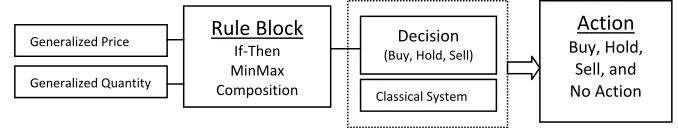
The system structure identifies the fuzzy rule based scheme so called fuzzy logic based inference flow from the input variables to the output variables. The fuzzification in the input interfaces translates crisp inputs into fuzzy values. The fuzzy inference system takes place in rule blocks which contain the linguistic control rules. The outputs of these rule blocks are linguistic variables. The defuzzification in the output interfaces translates them into analog variables.

The following table 1 shows the statistics of variables and rule blocks.

Input Variables 2

Output Variables 1

Rule Blocks 1

Rules 9 Membership Functions 9

Table 1. Statistics

The whole structure of this fuzzy system including input interfaces; rule blocks and output interfaces have been shown in Fig.1. The connecting lines symbolize the data flow.

Figure 1. Structure of Adaptive Fuzzy Rule Based Scheme

5.3. Variables and Parameters

Linguistic variables are used to translate real values into linguistic values. The possible values of a linguistic variable are not numbers but so called 'linguistic terms'.

Generalized Price

Generalized Quantity

Rule Block

If‐Then

MinMax

Composition

Decision (Buy, Hold, Sell)

Classical System

Action

(10)

164

Linguistic variables have to be defined for all input, output and decision variables. The membership functions are defined for linguistic variables.

The following table 2 lists all variables of the system.

L/Variables Fuzzy Numbers Parameter Fig. L/Variables

gPrice

(Low, Medium, High)

Z-Shaped for Low price Z (-0.85, -0.20)

Triangular for Medium price T (-0.62,0 ,0.1)

S-Shaped for High price S (0.05,0.6)

gQuantity

(Low, Medium, High)

Z-Shaped for Low quantity Z (-0.96,0.52)

Triangular for Medium quantity T (-0.15, 0, 0.1)

S-Shaped for High quantity S (0.075, 0.95)

gDecision

(Buy, Hold, Sell)

Buy for Triangular T (-1, -0.25,0.1)

Hold for Triangular T (0,0.25,0.5)

Sell for Triangular T (0.35,0.75,1)

Table 2. Linguistic variables and parameters

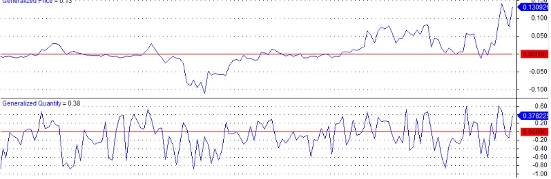
5.4. Generalized Price and Quantity

Generalized price and quantity of any stock are introduced by the equation

_t t t d, ; _t 0,

t

x x

X x t

x

−

= ≠ ∀ ∈ (5.1)

Here

x

t d, is the moving average of order d. Prices and quantities of stocks are transferred

to generalized prices and quantities by the Eq.(5.1). Fig.2 shows the generalized price and quantity of a stock.

Figure 2. Generalized price and quantity of a stock

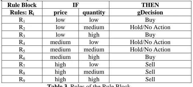
5.5. Rule Blocks

The rule blocks contain the control strategy of a fuzzy logic system. Each rule block confines all rules for the same context. A context is defined by the same input and output variables of the rules.

The rules ‘if’ part describes the situation, for which the rules are designed. The ‘then’ part describes the response of the fuzzy system in this situation.

(11)

165

rule block that combines the generalized price and generalized quantity to obtain a generalized decision. This rule block has been obtained according to the price and quantity spread analysis.

Rule Block IF THEN

Rules: Ri price quantity gDecision

R1 low low Buy

R2 low medium Hold/No Action

R3 low high Buy

R4 medium low Hold/No Action

R5 medium medium Hold/No Action

R6 medium high Buy

R7 high low Sell

R8 high medium Sell

R9 high high Sell

Table 3. Rules of the Rule Block 5.6. Operators

The fuzzy composition eventually combines the different rules to have a single conclusion. Minimum T-norm for if block, Mamdani for Implication and Maximum S-norm for Aggregation are used. Centroid defuzzification method has been applied to get crisp output. Different implication operators that may be used purposefully for a fuzzy rule based system [3].

5.7. Action

The generalized decision obtained from fuzzy rule based scheme is combined with ADX and Bollinger band indicators. ADX and Bollinger are technical indicators which are used for stock analysis [3,4]. If both systems agree at certain threshold action is taken to buy, sell, hold or no-action taken.

5.8. Data Description

Daily stock trading data of DSE (Dhaka Stock Exchange) have been collected from the website of stockbangldesh.com. Which contain opening, closing, high, low and quantity of stocks traded in a particular day. Data taken from DSE are used to convert generalized price and quantity Eq. (5.1). This generalized data are then fuzzified by fuzzy numbers. Table 2 shows the parameters of generalized prices and quantities. One of the most difficult tasks is to set the value of parameter of membership function. A statistical study has been made by taking more than 100 records of each company. The parameter value is accepted by the experts and general traders. Theorem 4.1, 4.2, 4.3, 4.6 and 4.7 claim that small changes or deviation of membership function, that is, the parameter value results in small change of conclusion.

5.9. Fuzzy Indicators

(12)

166 6. Results

Adaptive fuzzy rule based scheme have been implemented in some stock index. After having a buying decision stop loss, target profit and maximum holding day have been set. Table 4 shows few data that have been analysed by Adaptive Fuzzy Rule Based Scheme.

Table 4. HPR (holding period return) of some stock index

Figure 3. Decison (output) of the generealized prices and quantities of a stock input taken: gP=[-1 0 1 -1 -1 0 0 1 1] and gQ=[-1.5 0 1 0 1 -1.5 1 -1.5 0].

Stock Index Date Buy Stop Loss

Take Profit

Holding Duration

In day

Date: Sale/Short

HPR (Holding

period return)

Zahintex 30/6 28 -4 8 9 8/7:36 28%

GP 30/6 180 -10 20 10 15/7: 225 25%

KeyaCosmet 27/6 28 -3 6 9 7/7: 35 25%

Midasfin 9/6 30 -4 8 9 18/6: 40 33%

Lankabanfin 9/6 43 -3 6 10 18/6:55 27%

EnvoyTex 9/6 42 -5 10 9 20/6: 51 21%

Gpishpat 27/5 43 -4 8 9 6/6: 49 13%

Lafsurceml 27/5 31 -3 6 9 6/6: 34 9%

(13)

167

Figure 4. Buying and sellling state of geneeralized price and quantity of analyzed stock.

6.1. Conclusion

Many strategies are used for stock trading [4]. A trading system that always meets the trader’s expectation is hard to find. It is observed from Fig 3 that Adaptive fuzzy rule based scheme provides clean decision to buy, hold and sale. Table 4 describes the implemented result of this scheme that is very impressive. Fig 4 describes adaptive fuzzy rule based indicator that describes the region of buying and selling position.

Many stock data have been analyzed to compare the adaptive system by using the Amibroker and Matlab software package. The analysed result claims that the signal and result processed by adaptive fuzzy rule based scheme agrees with the result of technical indicators RSI, Stochastic [4,9-11]. It can be claimed that trading system with Adaptive fuzzy rule based scheme will provide satisfactory result. Automated trading system with adaptive fuzzy rule based scheme would have been a demanding toolkit for the investors.

Acknowledgement. The authors would like to thank for the cooperation of Prof. Dr. M. Dilder Hossain and Prof. Dr. Jahanara Begum Department of Basic Science, Primeasia University, Banani, Dhaka.

REFERENCES

1. R. Fuller, B. Werners, The compositional rule of inference with several relations, Tatra Mountains Math. Publ., 1 (1992), 39-44.

2. P.Henrici, Discrete Variable Methods in Ordinary Differential Equations, John Wiley & Sons, New York, 1962.

3. M. Shahjalal, Abeda Sultana, Nirmal Kanti Mitra and A.F.M. Khodadad Khan, Implementation of fuzzy rule based technical indicator in share market, International Journal of Applied Economics and Finance, 6 (2) (2012), 53-63.

4. S.B. Achelis, Technical Analysis from A to Z, 2ed., McGraw-Hill, New York, 2001. 5. E., Giovanis, E., Application of adaptive network-based fuzzy inference system in

macroeconomic variables forecasting, World Acad. Sci. Eng. Technol., 64 (2010), 660-667.

(14)

168

7. R. Fuller and H-J.Zimnermann, On Zadeh’s Compositional rule of inference, In: R.Lowen and M.Robunes., Fuzzy logic: State of the Art, Theory and decision Library, Series D, 1993, 193-200

8. R. Fuller and B. Werners, The compositional rule of inference with several relation, in: B.Riecan and M.Duchon eds., Proc. International Conference on Fuzzy sets and its Application, Liptovsky Mikulas, Czecho-Solvika, February 17-21, 1992, 39-44. 9. P. Dashore and S. Jain, Fuzzy rule based system to characterize the decision making

process: in share market, Int. J. Comput. Sci. Eng., 2 (2010), 1973-1979.

10. P. Thirunavukarasu, A study on share market situation: Fuzzy approach, Global J. Finance Manag., 1 (2009) 123-134.