ABSTRACT
CUFFNEY, LAURIE ANN. A Comparison of Threshold Parameters in DeterministicSIS and SI1I2S Models and StochasticSIS and SI1I2S Models. (Under the direction of John Franke.)
©Copyright 2013 by Laurie Ann Cuffney
A Comparison of Threshold Parameters in Deterministic SIS and SI1I2S Models and StochasticSIS and SI1I2S Models
by
Laurie Ann Cuffney
A thesis submitted to the Graduate Faculty of North Carolina State University
in partial fulfillment of the requirements for the Degree of
Master of Science
Applied Mathematics
Raleigh, North Carolina
2013
APPROVED BY:
Ralph Smith James Selgrade
John Franke
DEDICATION
BIOGRAPHY
ACKNOWLEDGEMENTS
I would like to thank my advisor Dr. John Franke for allowing me to work with him. His assistance was invaluable in the completion of this project.
I would also like to thank my committee members Dr. James Selgrade and Dr. Ralph Smith for agreeing to serve on my committee. Thank you for being a part of my committee and allowing this to all happen in a short time frame.
TABLE OF CONTENTS
LIST OF TABLES . . . vi
LIST OF FIGURES . . . vii
Chapter 1 Introduction . . . 1
Chapter 2 Literature Review . . . 3
Chapter 3 Stochastic one-stage SIS model . . . 9
3.1 Uniform parameters . . . 9
3.2 Poisson parameters . . . 12
3.3 Stochastic threshold parameter . . . 15
Chapter 4 Multi-Stage stochastic epidemic model . . . 18
4.1 Overview . . . 18
4.2 Numerical simulations . . . 19
4.3 Commuting matrices . . . 21
4.4 Non-commuting matrices . . . 27
Chapter 5 Conclusion . . . 32
References. . . 33
Appendix . . . 34
Appendix A Programs . . . 35
A.1 SIS Uniform . . . 35
A.2 Regression . . . 36
A.2.1 Endpoint search . . . 36
A.2.2 histmean function . . . 38
A.3 SI1I2S Uniform . . . 39
LIST OF TABLES
Table 2.1 Branching process SIS model where pjk Poisson with λ = α infected class mean of 1000 trails after 1000, 10000 and 100000 time steps. The deterministic R0 and approximate deterministic endemic equilibrium or disease free state are also given. . . 8
Table 3.1 Multiple trial run results for our stochastic SIS model with uniform pa-rameters. Infected class mean of 1000 trails after 1000, 10000 and 100000 time steps and deterministicRd
0. . . 11 Table 3.2 Approximation of the smallest value ofσmaxfor the interval [0, σmax] which
results in an endemic disease. The parameters α and σ follow a uniform distribution andα∈[0, αmax]. . . 11 Table 3.3 Approximation of the smallest value ofσmaxfor the interval [0, σmaxwhich
results in an endemic disease. The parameter α ∈ [0, αmax and α and σ follow a Poisson distribution. . . 14 Table 3.4 Multiple trial run results for our stochastic SIS model with poisson
pa-rameters. Infected class mean of 1000 trails after 1000, 10000 and 100000 time steps and deterministicRd
0 are shown. . . 14 Table 3.5 Stochastic epidemic model infected class mean of 1000 trails after 1000,
10000 and 100000 time steps with uniform parameters from various inter-vals. The deterministic Rd
0 and stochastic threshold Rs0 are given. . . 17
Table 4.1 Numerical examples of a stochastic SI1I2S model where α1 is uniform over the same interval as α2. Similarly the parameter σ1 is uniform over the same interval asσ2. The table contains the two infected class means of 1000 trails after 1000, 10000 and 100000 time steps with initial conditions S(0) = 99, I1(0) = 1, and I2(0) = 1. The deterministicRd0 is calculated using the means value of each parameter. . . 20 Table 4.2 Numerical examples of a stochastic SI1I2S model. Parameters α1, α2,
σ1 and σ2 are uniform over the interval given. The table contains the two infected class means of 1000 trails after 1000, 10000 and 100000 time steps with initial conditions S(0) = 99, I1(0) = 1, and I2(0) = 1. The deterministicRd
0 is calculated using the means value of each parameter. . . 22 Table 4.3 Comparison of the deterministic thresholdRd
0 and eigenvalues for matrix B and our choices for a commuting matrix;A1,A2,A3. . . 24 Table 4.4 Eigenvalues of natural logarithms of commuting matrix products. . . 27 Table 4.5 Numerical examples of a stochasticSI1I2S model. The parametersα1,σ1
andσ2 are fixed and parameterα2 is uniform over the given interval. The table contains the two infected class means of 1000 trails after 1000, 10000 and 100000 time steps with initial conditions S(0) = 99, I1(0) = 1, and I2(0) = 1. The deterministic Rd0 is calculated using the means value of each parameter.Rs
LIST OF FIGURES
Figure 2.1 Deterministic discrete-time multi-stageSI1I2S models with initial condi-tions N = 100, S(0) = 50, and I1(0) = 25 = I2(0) with parameters (a) α1 =−0.2, α2 = 0.3, σ1 = 0.5 , σ2 = 0.6 and (b) α1 = −0.8, α2 = 0.6, σ1 = 0.3 , σ2 = 0.5. The threshold parameter R0 for each model is; (a)
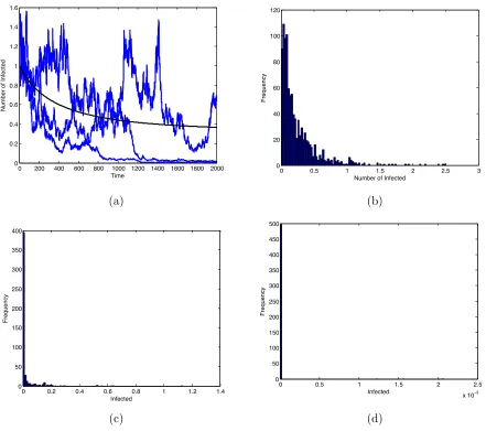
R0 = 3.8667, (b)R0= 0.9. . . 5 Figure 2.2 Parameter values α = .3, σ = .299; R0 = 1.003. Initial conditions
I(0) = 1,S(0) = 99. (a) Three sample paths of stochastic epidemic model versus deterministic model over 2000 time steps. Histograms showing fre-quency of infected individuals for 500 trials after (b) 1000 time steps; mean(I(t)) = 0.2528, (c)10000 time steps; mean(I(t)) = 0.0253 and (d) 100000 times steps; mean(I(t)) = 9.7275·10−6. . . 7
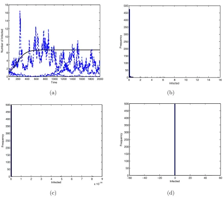
Figure 3.1 Initial conditionsI(0) = 1,S(0) = 99. (a) Three sample paths of stochas-tic epidemic model versus determinisstochas-tic model over 2000 time steps with uniform parameters α ∈ [0,0.3], σ ∈ [0,0.28]; R0 = 1.071428. (b)-(d) Uniform parameters α ∈ [0,0.8], σ ∈ [0,0.7233]; R0 = 1.1058. His-tograms showing frequency of infected individuals for 500 trials after (b) 1000 time steps; mean(I(t)) = 0.1365, (c)10000 time steps; mean(I(t)) = 2.6410·10−27 and (d) 100000 time steps; mean(I(t))) = 0. . . 10 Figure 3.2 Linear regression describing an approximate relationship between αmax
andσmaxwhenαandσfollow a uniform distribution. This line represents the dividing line between epidemic and disease free parameter sets. The regression is σ= 0.8235α+ 0.0365 with r2 = 0.9979. . . 12 Figure 3.3 Three sample paths of stochastic epidemic model versus deterministic
model over 2000 time steps. Parameters are Poisson with λ = .15 for α ∈[0,0.3] andλ=.14 forσ ∈[0,0.28]; R0 = 1.071428. . . 13 Figure 3.4 Linear regression of approximation relationship between the α max and
σ max. This line represents the dividing line between epidemic and dis-ease free parameter sets with Poisson parameters. The regression is σ = 0.9874α+ 0.0022 with r2 = 0.9999. . . 15 Figure 4.1 Initial conditions S(0) = 99, I1(0) = 1, I2(0) = 1 . Two sample paths
of a stochastic SI1I2S epidemic model 50 time steps. With commuting matrices B and (a)A1, (b)A2, and (c) A3. . . 23 Figure 4.2 Histogram of infected class means of 1,000 trial runs after 100,000 (a)
Chapter 1
Introduction
Epidemic models are used to predict disease spread through a population. Accurate prediction of disease spread is important in the management of outbreaks and treatment of disease. De-terministic discrete and continuous time models have a rich history of study and their behavior is well known [1, 3, 10, 15]. A simple deterministic discrete time SIS model with constant population is given by
S(t+ 1) =
1−αI
N
S+σI I(t+ 1) = αI
N S+ (1−σ)I (1.1)
whereαis the infection rate andσ is the recovery rate. The threshold parameter for this model comes from the basic reproduction number,
Rd 0=
α
σ. (1.2)
WhenRd
0 is less than one the disease is eradicated and the model goes to a disease free equilib-rium. IfRd
0 is greater than one the disease persists and spreads through the population [1, 5, 4]. The model (1.1) carries with it the inherent assumption that the infection rate, α, and the recovery rate, σ, are constant throughout the population and throughout time. In reality this assumption is flawed.
individual comes into contact with the same individual. Similarly an individual who is already sick has a higher likelihood to contract influenza when in contact with someone carrying the virus.
Discrete time epidemic models measure the spread of an epidemic at distinct time intervals i.e. days, months, or years. Over the course of time environmental changes may cause variation in the rate of infection and ability of infected individuals to recover. Changes in season and weather can cause a change in the rate of infection and ability to recover from illness. Thus the rate of infection and recovery are not constant.
To account for variation in infection rate and recovery rate over time we add stochasticity into our epidemic model. There are several approaches to introduce stochasticity into epidemic models. To introduce stochasticity the SIS model can be considered a Markov chain process where S and I are random variables [2, 3, 11]. Non-Markovian models have also been used to produce a stochastic epidemic model. In non-markovian models it may be the infectious rate and the infectious duration which generate stochasticity with in the model [6].
In this paper we will review a branching process model employed by Allen and Driessche [4] in chapter 2. We then outline a different method to introduce stochasticity into an epidemic model in chapter 3. In our model the parameters governing infection rate and recovery rate vary at each time step. The parameters follow a given distribution and are assumed to be i.i.d. We consider parameters which follow a uniform or Poisson distribution for numerical examples. Through numerical simulations we observe similar behavior to other stochastic epidemic models. When the deterministic thresholdRd
0 is greater than one, but close to one, we expect the disease to persist. However, the disease instead is effectively eradicated from the population. Through out this paper we make the consideration that if the disease is present in a very small portion of the population we will say the disease has been eradicated. If the number of infected is on the order of 10−5 or smaller we will consider this a disease free state.
To understand the behavior of our stochastic epidemic model we define a stochastic threshold parameter
Rs0 = E ln(α+ 1−σ)
Chapter 2
Literature Review
In this chapter we discuss a stochastic threshold and the threshold theorem introduced by Allen and van den Driessche [4]. We consider the discrete-time multi-stage model SI1. . . InS with constant population,
S(t+ 1) =
1− n X
j=1
αjIj(t) N
S(t) +σnIn(t)
I1(t+ 1) =
n X
j=1
αjIj(t) N
S(t) + (1−σ1)I1(t)
Ij(t+ 1) = (1−σj)Ij(t) +σj−1Ij−1, j = 2, . . . n. (2.1) In the multi-stage epidemic model we assume that individuals transition through stages follow-ing the schemeIj →Ij+1 forj= 1, ...n−1 andIn→S. Over one time step it is also assumed that an individual transitions only one stage further i.e. an individual in Ij at time t can only stay in Ij or transition to Ij+1.
Multi-stage models such as this can be used to model diseases that exhibit multiple con-tagious stages with different infection rates. An intermediate nonconcon-tagious stage can also be modeled by allowing the corresponding αi to be zero. We are interested in the behavior of the model near the disease free equilibrium. Linearization about the disease free equilibrium yields
I(t+ 1) =
α1+ 1−σ1 α2 · · · αn
σ1 1−σ2 0 · · · 0
0 σ2 1−σ3 0 · · ·
..
. ... . .. . .. ...
0 0 · · · σn−1 1−σn
where I(t) =
I1(t) .. . In(t) .
The matrix in (2.2) is a sum of two matrices Fd, the matrix of new infections, and Td, the transition matrix [4],
Fd =
α1 α2 · · · αn
0 0 0 0
.. . ... ... ... (2.3)
Td =
1−σ1 0 · · · 0
σ1 1−σ2 · · · 0
0 σ2 1−σ3 ... ..
. ... . .. ...
0 · · · σn−1 1−σn
. (2.4)
Using these two matrices we can build the next generation matrixKd=Fd(I−Td)−1[5]. The spectral radius of the next generation matrix provides the deterministic threshold R0=ρ(Kd) for the multi-stage discrete-time epidemic model (2.1). As with the single stage SIS model if the threshold parameter R0 is less than one the disease is eradicated. If R0 greater than one the disease persists within the population [4, 5]. In figure 2.1 we see two examples of anSI1I2S model with different parameters providing an example where R0 greater than one and and example where R0 less than one. In figure 2.1a the threshold parameter is R0 = 3.8667 which is greater than one and we see the disease is endemic as we would expect. For figure 2.1b the threshold parameter isR0= 0.9 which is less than one and we see the population recover from the initial infection and the disease die away over time.
To add stochasticity into this model we define the probability that one individual in the Ij class infectskindividuals in one time step. We notate this probability aspjk. The probabilities pjk follow some distribution over the interval [0,1] and
P∞
k=0pjk = 1. For the purposes of this paper we will generate pjk from a Poisson distribution, with mean λj =αj, or a uniform distribution. In this method the transition parameters, σi, remain constant.
We define the offspring probability generating functions near the disease free equilibrium as
hj(u) = ∞
X
k1=0
· · ·
∞
X
kn=0
Pj(k1, . . . , kn)uk11· · ·uknn (2.5)
produces k1 individuals in the I1 class, k2 individuals in the I2 class etc [4]. In this model due to imposed restrictions on movement between classes Pj(k1, . . . , kn) = 0 when ki ≥2 for any i≥2. Therefore the only nonzero probabilities we can have are Pj(k1, . . . , kn) where ki = 0,1 fori≥2.
Since we only allow an individual to either stay in the class or move to the next class, Pj(k1, . . . , kn) = 0 if ki = 1 for i6=j, j+ 1. This leaves the only potentail nonzero probabilities Pj(k1, . . . , kn) when ki = 0 for i = 1, j, j6 + 1 and either kj = 0 and kj+1 = 1 or kj = 1 and kj+1 = 0. Multiple new infected individuals may result from one infected individual so k1 is allowed to range from 0 to N. In practice this meansP3(k1, . . . , kn)= 0 for6 P3(k1,0,1,0, . . . ,0) andP3(k1,0,0,1,0, . . . ,0).P3(k1,0,1,0, . . . ,0) represents the probability that one individual in I3 stays in I3 and infects k1 individuals from the susceptible class successfully over one time step. Likewise the probabilityP3(k1,0,0,1,0. . . ,0) represents the individual moving fromI3to I4 and infectingk1 individuals from the susceptible class successfully over one time step.
To further simplify these probabilities we make the observation that new infections occur independently of transition between stages. Transmission of the disease from an infected indi-vidual to a susceptible indiindi-vidual occurs at the beginning of the time interval [4]. This means that the probabilities are independent and can be separated. Definerj(k) to be the probability that one infected individual in the jth class infects k individuals over one time step. Notice then rj(k) = pjk. Let qj(k2, . . . , kn) be the probability that in one time step one individual in thejth class produces k2 individuals in the I2 class, k3 individuals in the I3 class etc. We can
10 20 30 40 50 60 70 80 90 100 0 10 20 30 40 50 60 70 80 90 100 Time
Number of Individuals
S I1 I2
10 20 30 40 50 60 70 80 90 100
0 10 20 30 40 50 60 70 80 90 100 Time
Number of Individuals
S I1 I2
(a) (b)
now rewrite Pj(k1, . . . , kn) as
Pj(k1, . . . , kn) =pjk1·qj(k2, . . . , kn). (2.6)
We can define the probabilityqj for all values ofj as
qj(k2, . . . , kn) =
1−σj ifkj = 1,ki= 0 for i6=j σj ifkj+1 = 1,ki = 0 for i6=j+ 1 0 otherwise.
(2.7)
This simplifies (2.5) with respect to our model to
hj(u) = [(1−σj)uj+σjuj+1] ∞
X
k=0
pjkuk1, j= 1, . . . , n−1
hn(u) = [(1−σn)un+σn] ∞
X
k=0
pjkuk1. (2.8)
To describe this process we can calculate the expectation matrix Mdwhere,
mij = ∂hi ∂uj
u1=···=un=1[4].
The expectation matrixMdsatisfies the relationMdT = (Fd+Td). Allen and van den Driessche’s [4] threshold theorem states that ρ(Md) < 1(> 1) if and only if ρ(Kd) < 1(> 1). For this stochastic threshold when ρ(Md) less than one the process is subcritical and disease extinction occurs with probability one. Whenρ(Md) greater than one the process is supercritical and the probability of disease extinction is less than one. This means that if the deterministic threshold of the deterministic model with corresponding parameters to the stochastic model is less than one we are guaranteed to see disease extinction. When the corresponding deterministic threshold is greater then one we are not guaranteed to have an endemic. It is possible to have disease extinction even with the threshold parameter greater than one.
Consider the one stage model 1.1. The offspring probability generating function for this model is
h(u) = [(1−σ)u+σ1] ∞
X
k=0
pkuk (2.9)
disease free state. To determine the long term average behavior of the stochastic model we run numerical simulations for 1,000 trials at higher time steps. Figures 2.2b-d show the results of these simulations. We see through these histograms the average of the trials decreases over time and by the 100,000 time step have decreased to the point we will say the population is disease free. Here we see an instance of disease extinction where the deterministic threshold parameter isR0 = 1.003 which is greater than one.
0 200 400 600 800 1000 1200 1400 1600 1800 2000 0 0.2 0.4 0.6 0.8 1 1.2 1.4 1.6 Time
Number of Infected
0 0.5 1 1.5 2 2.5 3
0 20 40 60 80 100 120
Number of Infected
Frequency
(a) (b)
0 0.2 0.4 0.6 0.8 1 1.2 1.4
0 50 100 150 200 250 300 350 400 Infected Frequency
0 0.5 1 1.5 2 2.5
x 10−3 0 50 100 150 200 250 300 350 400 450 500 Infected Frequency (c) (d)
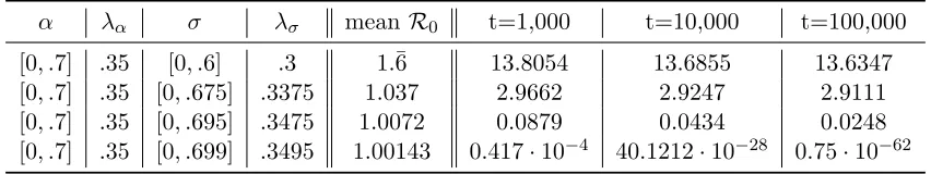
Table 2.1: Branching process SIS model where pjk Poisson with λ = α infected class mean of 1000 trails after 1000, 10000 and 100000 time steps. The deterministic R0 and approximate deterministic endemic equilibrium or disease free state are also given.
α σ t=1,000 t=10,000 t=100,000 R0 approx. equil.
0.3 0.27 9.5599 9.7901 9.8229 1.¯1 10
0.3 0.28 6.1755 6.4038 6.1256 1.07 6.¯6
0.3 0.29 2.8922 3.1253 3.1229 1.03 3.¯3
0.3 0.295 1.2102 1.2414 1.1722 1.01 1.¯6
0.3 0.297 0.6519 0.4646 0.6226 1.010¯ 1
0.3 0.298 0.5439 0.2407 0.1730 1.006 1.¯3 0.3 0.299 0.3571 0.0165 1.5376·10−9 1.003 0.¯6 0.3 0.3 0.1559 7.6995·10−5 1.8547·10−48 1 0 0.3 0.35 2.8608·10−23 1.6871·10−235 4.9407·10−334 0.857 0
Chapter 3
Stochastic one-stage SIS model
Expanding on the previous work in chapter one we allow the parameters governing infection rate and recovery rate to both follow some distribution. For simplification the model parameters are i.i.d. and we consider only the Poisson and uniform distribution. In this chapter we will focus on the one-stage model (1.1).
3.1
Uniform parameters
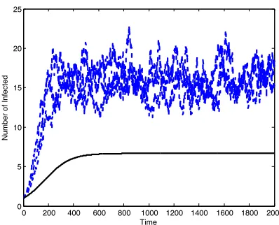
Assume that the parameters α and σ follow a uniform distribution over a given interval. In figure 3.1a we numerically simulate three sample paths for anSIS model with both parameters allowed to vary. At first we may assume the deterministic threshold (1.2) using the mean ofα and the mean of σ to be an accurate stochastic threshold parameter. We see in figure 3.1 two examples of when this threshold fails to hold true in practice.
In figure 3.1a α∈[0,0.3] andσ ∈[0,0.28] are uniform. At time t= 1600 one of the sample paths goes to zero even though the deterministic threshold parameterRd
0 = 1.071428 is greater than one suggesting an endemic disease. Figures 3.1b-d show the frequency of the number of infected individuals for 500 trials at different time steps for the stochastic SIS model with uniform parameters α ∈ [0,0.8], σ ∈ [0,0.7233]. As time increases the average over 500 trials decreases and the disease presence in the population decreases to the extent we are comfortable saying the disease has effectively been eradicated even though the deterministic threshold is greater than one. Table 3.1 shows results for the mean of the I class after time steps 1000, 10000, and 100000 and the deterministic threshold (1.2) calculated using the mean of each parameter.
that the ratio ασ is greater than one at one time step and less than one at another time step is zero. The ratio ασ is either always greater than one or always less than one. When the two intervals overlap it is possible for the ratio ασ to be greater than one at one time step and less than one at another time step. The question then is at what point does the overlap cause the stochastic model to become disease free when we would expect based on the means to have an endemic disease.
0 200 400 600 800 1000 1200 1400 1600 1800 2000 0 2 4 6 8 10 12 14 16 18 Time
Number of Infected
0 2 4 6 8 10 12 14 16
0 50 100 150 200 250 300 350 400 450 500 Infected Frequency (a) (b)
0 1 2 3 4 5 6 7 8 9
x 10−25 0 50 100 150 200 250 300 350 400 450 500 Infected Frequency
−60 −40 −20 0 20 40 60
0 50 100 150 200 250 300 350 400 450 500 Infected Frequency (c) (d)
To answer this question we run simulations with theαinterval fixed and vary theσ interval. For all simulations the intervals are of the form [0, αmax] and [0, σmax]. To find the smallestR0 that shows a disease epidemic we compare the mean values for 1,000 trials at the time steps 100,000 and 300,000. If the mean at 300,000 differs from the mean at 100,000 by a factor of 30 and neither mean is on the order of 1×10⁻⁵ we say there is an epidemic. If either of the means is less than or equal to 1×10⁻⁵ or the means differ by more than a factor of 30 we say that the model is approaching a disease free equilibrium. Refer to Appendix A.2 for a detailed view of the program. This is repeated for theαendpoints 0.2,0.3, . . . ,1. The results of this experiment
Table 3.1: Multiple trial run results for our stochastic SIS model with uniform parameters. Infected class mean of 1000 trails after 1000, 10000 and 100000 time steps and deterministic
Rd 0.
α σ Rd
0 t=1,000 t=10,000 t=100,000 [0, .4] [.5, .7] 0.¯3 1.1506·10−227 0 0 [.3, .4] [.1, .2] 2.¯3 34.1231 34.3557 34.0874 [.4, .6] [.35, .55] 1.¯1 5.5527 5.6389 5.5010 [.3, .7] [.25, .65] 1.¯1 6.5698 6.9806 7.4433 [.2, .8] [.25, .75] 1.¯1 2.6205 3.1808 3.9760 [.4, .6] [.3, .5] 1.25 19.1799 19.3276 19.8807 [.3, .7] [.3, .5] 1.25 18.1380 18.3112 18.1623 [0, .5] [0, .4] 1.25 13.6954 14.3214 14.3711 [0, .5] [0, .47] 1.0638 0.3614 1.4550·10−5 7.1654·10−169
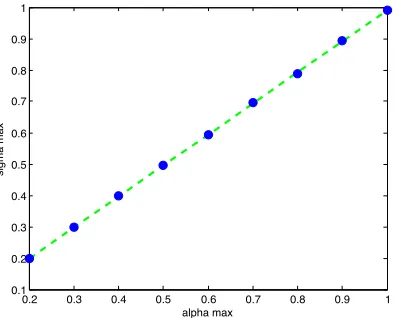
Table 3.2: Approximation of the smallest value of σmax for the interval [0, σmax] which results in an endemic disease. The parametersα andσfollow a uniform distribution and α∈[0, αmax].
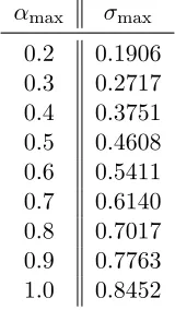
0.2 0.3 0.4 0.5 0.6 0.7 0.8 0.9 1 0.1
0.2 0.3 0.4 0.5 0.6 0.7 0.8 0.9
alpha max
sigma max
Figure 3.2: Linear regression describing an approximate relationship between αmax and σmax when α and σ follow a uniform distribution. This line represents the dividing line between epidemic and disease free parameter sets. The regression is σ = 0.8235α+ 0.0365 with r2 = 0.9979.
are show in table 3.2.
From this data we find the linear regression shown in figure 3.2 given byσ= 0.8235α+0.0365. In the deterministic case the slope of this line would be one. We see here that by adding stochasticity into our model the behavior of the threshold parameter changes. If theα interval and the σ interval both begin at zero and the choice for αmax and σmax give a point above the line in figure 3.2 we should expect the disease be eradicated over time. If the choice of αmax and σmax is below the line we expect the disease to persist.
3.2
Poisson parameters
Using the same approach as the uniform distribution we examine similar experiments for the model (1.1) with parameters that follow a Poisson distribution. Figure 3.3 shows three sample paths for the stochastic model with Poisson parameters α and σ. The parameter ranges are the same as those in figure 3.1. Comparing these two images we can see that a shift has occurred when we change from uniform to Poisson. Intervals which produced a disease free result with uniform parameters may produce an endemic result when the parameters follow Poisson distribution. Based on the difference between figure 3.1 and figure 3.3 we predict an increase in the σmax endpoint of the interval [0, σmax] when we run simulations to generate a table for poisson parameters similar to table 3.2.
0 200 400 600 800 1000 1200 1400 1600 1800 2000 0
5 10 15 20 25
Time
Number of Infected
Figure 3.3: Three sample paths of stochastic epidemic model versus deterministic model over 2000 time steps. Parameters are Poisson withλ=.15 forα∈[0,0.3] andλ=.14 forσ∈[0,0.28];
R0 = 1.071428.
poisson parameters. For all simulations the intervals are of the form [0, αmax] and [0, σmax].The approximated values for the smallestσmaxin theσinterval [0, σmax] are show in table 3.3. Look-ing at the values in table 3.3 and comparLook-ing them to the values found for uniform distributions in table 3.2 we can see that value for σmax has increased for allαmax as we predicted.
This occurs because the Poisson distribution is concentrated near the mean and the proba-bility of hitting a value far from the mean is small. In the uniform distribution the probaproba-bility is equal for all values in the interval. This means that the overlap for the two intervals describing α and σ may be larger for Poisson parameters then uniform parameters before we encounter a deterministic thresholdRd
0 greater than one but see disease eradication in practice. The linear regression, figure 3.4, σ = 0.9874α+ 0.0022 with r2 = 0.9999 shows a visible increase in the α coefficient of the regression from uniform to poisson. As before if the α interval and the σ interval both begin at zero and the choice for αmax and σmax give a point above the line in figure 3.4 we should expect the disease be eradicated over time. If the choice of αmax andσmax is below the line we expect the disease to persist.
Table 3.3: Approximation of the smallest value ofσmax for the interval [0, σmax which results in an endemic disease. The parameter α∈[0, αmaxand α and σ follow a Poisson distribution.
αmax σmax 0.2 0.1986 0.3 0.2988 0.4 0.3977 0.5 0.4966 0.6 0.5943 0.7 0.6958 0.8 0.7876 0.9 0.8923 1.0 0.9899
Table 3.4: Multiple trial run results for our stochastic SIS model with poisson parameters. Infected class mean of 1000 trails after 1000, 10000 and 100000 time steps and deterministic
Rd
0 are shown.
3.3
Stochastic threshold parameter
It is apparent that the deterministic threshold does not accurately predict the behavior of our stochastic model . To descibe the long term behavior of our stochastic model we must establish a new stochastic threshold. We adapt the ideas of Lewontin and Cohen[12] from population models to epidemic models to build our stochastic threshold. The linearization of (1.1) is
I(t+ 1) = (α+ 1−σ)I(t). (3.1)
In the deterministic model we can rewrite this linearization as
I(n) = (α+ 1−σ)nI(0). (3.2) In our stochastic model the parametersα and σ vary over time and the coefficient (α+ 1−σ) is different at each time step. Thus the linearization for the stochastic model is
I(n) = α(n) + 1−σ(n)· · · α(1) + 1−σ(1)I(0) (3.3) whereα(i) andσ(i) are the values of the parametersαandσat timei. The parametersαandσ are assumed to be i.i.d. and have finite mean since 0≤α, σ≤1. This means that if we consider a new parameter li=α(i) + 1−σ(i), theli are i.i.d. and also have finite mean. To show there is disease persistence in the model we need to know the probability that limt→∞I(t) greater
0.2 0.3 0.4 0.5 0.6 0.7 0.8 0.9 1
0.1 0.2 0.3 0.4 0.5 0.6 0.7 0.8 0.9 1
alpha max
sigma max
than zero. In our model since the population is constant we first consider the probability
P r{A≤I(n)≤B} (3.4)
where 0< A, B < N andN is the total population. Since the natural logarithm is a monotone function we can say
P r{A≤I(n)≤B}=P r{ln(A)≤ln(I(n))≤ln(B)} [12]. (3.5) For our model
ln(I(n)) = ln h
α(n) + 1−σ(n)· · · α(1) + 1−σ(1)
I(0) i
(3.6)
which can be simplified to
ln(I(n)) = n X
i=1
ln α(i) + 1−σ(i)
+ ln I(0) =
n X
i=1
ln(li) + ln I(0)
. (3.7)
We substitute this into (3.5) and simplify to get
P r{A≤I(n)≤B}=P r ( ln A I(0) ≤ n X i=1
ln(li)≤ln
B I(0)
)
[12]. (3.8)
We can take the time average of the right hand side of (3.8) to get
P r{A≤I(n)≤B}=P r 1 nln A I(0)
≤ln(li)ˆ ≤ 1
nln B I(0) (3.9)
where ln(lˆi) is the arithmetic mean of ln(li) over n time steps[12]. Since we have already es-tablished the li are i.i.d. and have finite mean then ln(li) has mean µln(li) and variance ρln(li)
the Central Limit Theorem tells us that ln(lˆi) over large samples is normally distributed with mean µln(li) and varianceρln(li)[12]. Lewontin and Cohen[12] define the values
τ1 = 1 nln A I(0)
−µln(li)
ρln(li)/
√
n , τ2 = 1 nln B I(0)
−µln(li)
ρln(li)/
√
n , (3.10)
so that
Asτ1 grows the normal integral betweenτ1 andτ2 shrinks and approaches zero. This means if µln(li) is less than zero the model approaches a disease free equilibrium. Ifµln(li)is greater than
zero the disease persists over time with in the population[12]. We use these results by Lewontin and Cohen[12] to build a stochastic threshold parameter for our model.
We define this new threshold as
Rs
0= E(ln(α+ 1−σ)). (3.12)
IfRs
0is less than zero we expect our stochasticSISmodel to approach a disease free equilibrium If Rs
0 is greater than zero we expect the disease to persist over time. This type of threshold parameter has been employed previously in work on populations models but has yet to find prominence in the application to disease models [9, 7, 12, 13]. This new threshold parameter allows us see a clearer picture of the behavior of the stochastic model over time.
Table 3.5 demonstrates the improvement over the deterministic threshold Rd
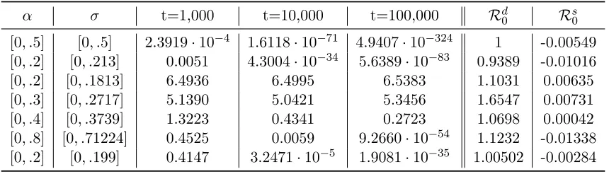
0 by using the new stochastic threshold parameter Rs
0. One important example given in table 3.5 is when α ∈ [0, .8] and σ ∈[0, .71224]. In this example Rd
0 is greater than one which tells us that the disease may remain in the population. The numerical simulation in table 3.5 show the model goes to what we consider a disease free state. In table 3.5 we see that Rs
0 is less than zero which agrees with what we see numerically. Using this new threshold parameter we can more accurately predict the behavior of our stochastic model.
Table 3.5: Stochastic epidemic model infected class mean of 1000 trails after 1000, 10000 and 100000 time steps with uniform parameters from various intervals. The deterministic Rd
0 and stochastic threshold Rs
0 are given.
α σ t=1,000 t=10,000 t=100,000 Rd
0 Rs0
Chapter 4
Multi-Stage stochastic epidemic
model
4.1
Overview
To further expand this model we now incorporate our stochastic parameters into the multi-stage model (2.1). In this model each parameterαi andσi for,i= 1, . . . , n, is i.i.d. and follow a uniform distribution. If we wish to apply our threshold parameter from chapter 3 we consider the linearization (2.2). In the one stage model the form of the I(t) coefficient allowed us to simplify (3.1) to (3.2). In the multistageSI1· · ·InS model linearization (2.2) theI(t) coefficient is
L=
α1+ 1−σ1 α2 · · · αn
σ1 1−σ2 0 · · · 0
0 σ2 1−σ3 0 · · ·
..
. ... . .. . .. ...
0 0 · · · σn−1 1−σn
. (4.1)
This raises several questions. If we approach building a new threshold parameter in the same way we have
Rs
0 = E(ln(Ln· · ·L1)). (4.2) This would result in a matrix valued threshold parameter. This does not provide us the infor-mation we desire so we have to adapt the threshold parameter to the multi-stage model. We would like to adapt the threshold parameter in a way that preserves the integrity of the our threshold parameter for the single stage model (3.12).
stage models carries over into multi-stage models. Here we consider the two stageSI1I2S model
S(t+ 1) =
1−α1I1(t)
N −
α2I2(t) N
S(t) +σ2I2(t)
I1(t+ 1) =
α1I1(t)
N +
α2I2(t) N
S(t) + (1−σ1)I1(t)
I2(t+ 1) = σ1I1(t) + (1−σ2)I2(t). (4.3)
The linearization of the two stage SI1I2S model is
I(t+ 1) = α1+ 1−σ1 α2 σ1 1−σ2
!
I(t). (4.4)
The deterministic threshold parameterR0 =ρ(Kd) for (4.3) is
Rd 0 =
α1 σ1
+ α2 σ2
. (4.5)
For the two stage model the matrixL is
L= α1+ 1−σ1 α2 σ1 1−σ2
!
. (4.6)
Unlike before the linearization does not simplify nicely. Because we are now dealing with ma-trices it is important to realize that at each time step the entries within matrixL change and as a resultLi may not commute withLi+1 for any i. We can write our model as
I(n) =LnLn−1· · ·L1I(0) (4.7)
where Li is the matrix (4.6) at time i. Where we were previously able to simplify the natural logarithm we can not because the matrices do not commute and ln(AB) = ln(A) + ln(B) only if the matrices Aand B commute.
4.2
Numerical simulations
interval choices and also provides the deterministic threshold calculated using the parameter means.
As we would expect the our stochastic model may go to a disease free equilibrium when the deterministic threshold based on parameter means is greater than one. An interesting obser-vation we can make from these numerical examples is that when σmax approaches twiceαmax we have a deterministic threshold greater one but in practice the model goes to a disease free equilibrium. The deterministic threshold (4.5) simplifies to
Rd0 = 2µ(α1) µ(σ1)
(4.8)
Table 4.1: Numerical examples of a stochasticSI1I2Smodel whereα1is uniform over the same interval as α2. Similarly the parameter σ1 is uniform over the same interval as σ2. The table contains the two infected class means of 1000 trails after 1000, 10000 and 100000 time steps with initial conditionsS(0) = 99, I1(0) = 1, and I2(0) = 1. The deterministic Rd0 is calculated using the means value of each parameter.
α1,α2 σ1,σ2 t=1,000 t=10,000 t=100,000 Rd0 [0,0.2] [0,0.35] 5.2626 5.2272 5.3399 1.14286 [0,0.2] [0,0.39] 0.1602 0.4413·10−5 0.5925·10−92 1.02564 [0,0.3] [0,0.5] 6.9422 6.9458 7.0635 1.2 [0,0.3] [0,0.59] 0.1362 1.0224·10−4 8.0984·10−119 1.01695 [0,0.3] [0,0.6] 0.0280 1.2046·10−12 6.1544·10−270 0.9836 [0,0.4] [0,0.75] 0.9871 0.8282 0.9618 1.0¯6 [0,0.4] [0,0.78] 0.0719 5.9337·10−13 1.5511·10−215 1.0256 [0,0.4] [0,0.8] 0.0015 0.2566·10−42 0 1
(a) I1
α1,α2 σ1,σ2 t=1,000 t=10,000 t=100,000 Rd0 [0,0.2] [0,0.35] 5.3874 5.2678 5.2922 1.14286 [0,0.2] [0,0.39] 0.1616 0.3554·10−5 0.5125·10−92 1.02564 [0,0.3] [0,0.5] 6.9852 6.9737 6.9994 1.2 [0,0.3] [0,0.59] 0.1386 9.8186·10−5 5.8915·10−119 1.01695 [0,0.3] [0,0.6] 0.0250 1.7066·10−12 2.6788·10−270 0.9836 [0,0.4] [0,0.75] 0.9576 0.7957 0.8449 1.0¯6 [0,0.4] [0,0.78] 0.0777 1.2560·10−12 9.3813·10−216 1.0256 [0,0.4] [0,0.8] 0.0013 0.2468·10−42 0 1
sinceα1 and α2 are over the same interval they have the same mean,µ(α1). The same can be said of the parameters σ1 and σ2. Thus for the deterministic threshold Rd0 to equal one µ(σ1) must be greater than or equal to twice µ(α1). Since we expect to see disease extinction when the deterministic threshold is greater one is is not surprising to see the shift happen whenσmax close to twiceαmax.
For our next set of numerical simulations we assign an interval to each parameter and observe the behavior of each infected class over time. These simulations are shown in table 4.2. We see that more most of our simulations the deterministic threshold Rd
0 is a good indicator of the model behavior. The simulations of interest in table 4.2 are the last three simulations. In these simulations the parametersα1,σ1 and σ2 are uniform over the same interval for all three trials. The σ1 interval is the only change between simulations. Looking at these three simulations we see the deterministic thresholdRd
0 decrease and the behavior of the model switch from disease persistence to disease extinction. Whenσ1∈[0,0.55] the deterministic threshold is greater than one but the model goes to a disease free state.
4.3
Commuting matrices
To simplify our analysis we now consider the rare case where the matrices Li do commute. Commuting matrices provide a simple example since (4.2) can now be simplified to,
Rs0 = E n X
i=1 ln(Li)
!
. (4.9)
If we follow the same basic argument and take the time average we can express the threshold parameter more simply as
Rs0= E ln(L). (4.10)
ThisRs
0 is matrix valued and does not provide the information we want for the model. To cope with this issue we observe the eigenvalues for the matrices.
First we must find commuting matrices that satisfy the conditions on the parameters αi and σi, 0≤α1, α2, σ1, σ2 ≤1. Choose a matrixB,
B= 0.7 0.2 0.8 0.5
!
(4.11)
whereα1 = 0.5,α2= 0.2,σ1 = 0.8 andσ2= 0.5. If we consider this matrix in the deterministic model Rd
The first commuting matrix we chose is
A1=
0.3 0.2 0.8 0.1
!
(4.12)
whereα1 = 0.1,α2= 0.2,σ1 = 0.8 andσ2= 0.9. If we consider this matrix in the deterministic modelRd
0 = 0.34722 and the disease is eradicated. We now have two commuting matrices with different deterministic Rd
0 values. The product of these two matrices
BA1 =
0.37 0.16 0.64 0.21
!
(4.13)
has a deterministicRd
0 = 0.2181566.
We use these two matrices to generate a simple stochastic SI2I2S model by randomly
Table 4.2: Numerical examples of a stochastic SI1I2S model. Parameters α1, α2, σ1 and σ2 are uniform over the interval given. The table contains the two infected class means of 1000 trails after 1000, 10000 and 100000 time steps with initial conditionsS(0) = 99,I1(0) = 1, and I2(0) = 1. The deterministic Rd0 is calculated using the means value of each parameter.
α1 α2 σ1 σ2 t=1,000 t=10,000 t=100,000 Rd0
[0.2,0.3] [0.3,0.4] [0,0.2] [0,0.2] 41.6579 41.5514 41.5605 6
[0,0.2] [0,0.2] [0.6,0.8] [0,0.5] 0.1150·10−49 0 0 0.54285
[0,0.1] [0,0.5] [0,1] [0,1] 5.3272·10−61 0 0 0.6
[0,0.2] [0.4,0.6] [0,0.25] [0,0.8] 38.0228 38.3215 38.1930 2.05
[0,0.2] [0.4,0.6] [0,0.6] [0,0.8] 19.8131 19.8854 19.7090 1.58¯3
[0,0.2] [0,0.6] [0,0.6] [0,0.8] 1.9263 1.9943 2.0670 1.08¯3
[0,0.2] [0,0.55] [0,0.6] [0,0.8] 0.1454 2.4367·10−5 2.7525·10−151 1.02083
[0,0.2] [0,0.4] [0,0.6] [0,0.8] 8.5438·10−16 2.0028·10−176 0 0.8¯3
(a) I1
α1 α2 σ1 σ2 t=1,000 t=10,000 t=100,000 Rd0
[0.2,0.3] [0.3,0.4] [0,0.2] [0,0.2] 41.4177 41.4582 41.4795 6
[0,0.2] [0,0.2] [0.6,0.8] [0,0.5] 0.6163·10−49 0 0 0.54285
[0,0.1] [0,0.5] [0,1] [0,1] 6.4059·10−61 0 0 0.6
[0,0.2] [0.4,0.6] [0,0.25] [0,0.8] 12.1596 11.6508 11.8227 2.05
[0,0.2] [0.4,0.6] [0,0.6] [0,0.8] 14.7394 14.8360 15.1986 1.58¯3
[0,0.2] [0,0.6] [0,0.6] [0,0.8] 1.4257 1.5367 1.5173 1.08¯3
[0,0.2] [0,0.55] [0,0.6] [0,0.8] 0.1028 4.7676·10−5 2.8302·10−151 1.02083
[0,0.2] [0,0.4] [0,0.6] [0,0.8] 8.9781·10−16 2.4334·10−176 0 0.8¯3
choosing which of the two matrices to apply at each time step. Each of the two matrices has equal probability, 12, of being applying at any time step. Figure 4.1a shows two sample runs of the model (4.3) with the commuting matrices A1 and B. In the case of these choices for commuting matrices the model goes disease free.
We can calculate the expected value for the matrix L at each time step. In this case there are only two possibilities each of equal probability, 12, i.e. at each time step L=B or L=A1.
0 5 10 15 20 25 30 35 40 45 50
0 0.2 0.4 0.6 0.8 1 1.2 1.4
Time
Infected
I1 I2
0 5 10 15 20 25 30 35 40 45 50
0.7 0.8 0.9 1 1.1 1.2 1.3 1.4
Time
Infected
I1 I2
(a) (b)
0 5 10 15 20 25 30 35 40 45 50
0.5 0.6 0.7 0.8 0.9 1 1.1 1.2 1.3 1.4
Time
Infected
I1 I2
(c)
Table 4.3: Comparison of the deterministic thresholdRd
0 and eigenvalues for matrixBand our choices for a commuting matrix; A1,A2,A3.
Matrix ρ Rd
0
B 1.01231 1.025
A1 0.612311 0.34722 BA1 0.619848 0.2181566 1
2(B+A1) 0.812311 0.66071 A2 0.992311 0.98461 BA2 1.00453 1.0077 1
2(B+A2) 1.00231 1.0046 A3 0.987811 0.97569 BA3 0.999971 0.99995 1
2(B+A3) 1.00006 1.001219
The expectation matrix is E(L) = 12(A1+B),
E(L) = 0.5 0.2 0.8 0.3
!
. (4.14)
If we consider this matrix for a deterministic model the parameters are α1 = 0.3, α2 = 0.2, σ1 = 0.8 andσ2= 0.7 with R0 = 0.6671.
To investigate the threshold parameter we calculate the eigenvalues for the matricesB,A1, BA1, and E(L). We see in table 4.3 for B the deterministic threshold Rd0 is greater than one and the spectral radius ρ(B) = 1.01231 is greater than one. Similarly we see for matrices A1 and BA1,Rd0 is less than one and the spectral radius for these matrices is also less than one. For this example the behavior of the stochastic model aligns with the deterministic threshold for the product matrix BA1 and the deterministic threshold for the expectation matrix.
Consider a different commuting matrix
A2=
0.68 0.2 0.8 0.48
!
(4.15)
where α1 = 0.48, α2 = 0.2,σ1 = 0.8 and σ2 = 0.52. The deterministic model for A2 is disease free with Rd
deterministic behavior. Their product
BA2 =
0.636 0.236 0.944 0.4
!
(4.16)
Rd
0 = 1.0077 so the disease is endemic. With this choice of commuting matrices we have two matrices with different deterministic behavior whose product results in a model with endemic behavior. The previous choice for a commuting matrix also had different deterministic behavior thanB but the product resulted in a disease free model. This shows that it is possible to mix matrices with different deterministic behavior and get either a disease free or epidemic result.
We can calculate the expected value for the matrix L at each time step. In this case there are only two possibilities each of equal probability, 12, i.e. at each time step L=B or L=A2. The expectation matrix is E(L) = 12(A2+B),
E(L) = 0.69 0.2 0.8 0.49
!
. (4.17)
If we consider this matrix for a deterministic model the parameters are α1 = 0.49, α2 = 0.2, σ1 = 0.8 andσ2= 0.51 with R0 = 1.00231.
Figure 4.1b shows two trial runs of (4.3) with commuting matrices A2 and B. In this case it is harder to see the behavior of the stochastic model. To investigate the long term behavior of the model we run a larger number trials over large time steps to determine the expected behavior. In figure 4.2 the mean value of I1 over 1,000 trials is 0.1763 at 100,000 time steps. After 300,000 times steps the mean value of I1 is 0.1752. The difference between the mean at 100,000 times steps and 300,000 times steps is small enough that we say there is an epidemic. We observe a similar variation in theI2 mean at 100,000 and 300,000. The spectral radius for A2, ρ(A2) = 0.98461 is less than one and for the product matrix BA2, ρ(BA2) = 1.00453 is greater than one and agrees with the deterministic threshold forA2 andBA2 as we see in table 4.3. The deterministic threshold for the expectation matrix is also greater than one.
The previous two examples give the false impression that the stochastic threshold param-eter is equivalent to the dparam-eterministic threshold paramparam-eter of the expectation matrix or the deterministic threshold of the product matrix. To show this does not hold for all commuting matrices consider the matrix
A3 =
0.6755 0.2 0.8 0.4755
!
(4.18)
trial runs of (4.3) with commuting matrices B and A3. After 50 time steps the behavior of the stochastic model is unclear. In figure 4.3 we observe I1 and I2 after 100,000 and 300,000 time steps and 1,000 trials. After 100,000 and 300,000 time steps there is a noticeable shift in theI2 mean from 0.0016 to 4.8823·10−4. After 300,000 times steps the infected class means are small enough we say the disease has been effectively eradicated and the model goes to a disease free state.
The product matrix for B and A3
BA3=
0.63285 0.2351 0.9404 0.39775
!
(4.19)
where α1 = 0.57325, α2 = 0.2351, σ1 = 0.9404 and σ2 = 0.60225 with deterministic R0 = 0.99995.
We can calculate the expected value for the matrix L at each time step. In this case there are only two possibilities each of equal probability, 12, i.e. at each time step L=B or L=A3. The expectation matrix is E(L) = 12(A3+B),
E(L) = 0.68775 0.2 0.8 0.48775
!
. (4.20)
If we consider this matrix for a deterministic model the parameters areα1 = 0.48775,α2= 0.2, σ1 = 0.8 andσ2= 0.51225 with R0 = 1.001219.
In this example we encounter the first disagreement between the deterministic threshold for the product matrix and the deterministic threshold for the expectation matrix. The deter-ministic threshold for the product matrix points to the stochastic model approaching a disease free state. The expectation matrix threshold predicts an endemic disease state for the model. In our numerical examples we observe that the model with commuting matricesA3 andB goes to a disease free state. This tells us that the expectation matrix is not a good indicator of the behavior of the stochastic model.
In this overly simplified model it appears as though an appropriate threshold would be
Rs0 = E(ρ(AB)). (4.21)
Table 4.4: Eigenvalues of natural logarithms of commuting matrix products.
Matrices λ1 λ2
ln(BA1) −0.4782 + 7.6478·10−10i −3.2267 + 3.14159i
ln(BA2) 0.0045 -3.458608
ln(BA3) -0.0000029 -3.4858101
In the deterministic model we utilize the spectral radius to describe the overall behavior of the model. In a similar fashion we look at the eigenvalues of the product matrixBAi and look at the maximum eigenvalue instead of the maximum absolute value. Letλ1 andλ2 be the eigenvalues of the matrixL. We can rewrite (4.10) as
Rs0= E (max{Real(λ1),Real(λ2)}). (4.22)
where Real(λi) is the real part of λi. Table 4.4 shows the results for this threshold parameter with our three choices of commuting matrices. We see based on the table that when the real part of the largest eigenvalue is less than zero the model goes to a disease free state and when it is greater than zero the disease persists within the population. Now that we have an idea for the two-stage model in a simplified case we investigate the reliability of the threshold in a more complex setting.
4.4
Non-commuting matrices
Consider now the case where we are not guaranteed that any of the matrices Li commute. Our argument for the threshold parameter (4.22) now breaks down since we can no longer simplify the natural logarithm of the productLn· · ·L1. Through numerical simulations we can see that the inability to simplify the natural logarithm nullifies the usability of the threshold parameter (4.22). In theSI1I2Smodel we now choose each parameter randomly at time t based on a distribution. This changes the way we calculate the expected value. First we calculate the eigenvalues of ln(L) in the two-stage model,
λ1,2= ln
1 2
r+ 1−σ2±
p
(σ2−1−r)2−4(r−rσ2−α2σ1)
. (4.23)
To simplify our calculations we consider the case where the parameters α1,σ1, and σ2 are fixed and we allow only α2 to vary over time. In table 4.5 we see the mean of the I1 and I2 classes as time progress in comparison to both the deterministic threshold, calculated using the parameter means, and our theoretical stochastic threshold (4.22). In this table we see that (4.22) correctly predicts the model behavior for most cases including several which have deterministic threshold greater than one but go to a disease free equilibrium. The case of interest is when α2 ∈[0,0.85] where the numerical simulation shows the disease persisting in the population but
Rs
0 is less than zero. This occurs because our choice ofRs0 require that the matrices commute which is not true.
We see that when the deterministic threshold is close to oneRs
0is not reliable. The threshold
Rs
0 passes zero and changes sign earlier then it should. Since Rs0 is an increasing function we can conclude that it accurately predicts behavior when the deterministic threshold is less than 1. Once the deterministic threshold is greater than 1 Rs
0 may become inaccurate. However as the deterministic threshold increases from 1 there is a higher likely hood thatRs
0 describes the model.
Table 4.5: Numerical examples of a stochasticSI1I2S model. The parametersα1,σ1andσ2are fixed and parameter α2 is uniform over the given interval. The table contains the two infected class means of 1000 trails after 1000, 10000 and 100000 time steps with initial conditions S(0) = 99, I1(0) = 1, andI2(0) = 1. The deterministic Rd0 is calculated using the means value of each parameter.Rs
0 is the expectation of the maximum of the real part of the eigenvalues of L.
α1 α2 σ1,σ2 t=1,000 t=10,000 t=100,000 Rd0 Rs0
0 .4 [0,0.2] σ1=.4,σ2=.5 9.2080 9.1498 9.1775 1.2 0.010518
0 .4 [0,0.3] σ1=.4,σ2=.5 12.7051 12.6299 12.6808 1.3 0.02727
0 .4 [0,0.5] σ1=.4,σ2=.5 18.2603 18.2938 18.3252 1.5 0.671718
0 .4 [0,1] 0.8 4.0182 4.1669 4.3129 1.125 0.01537
0 .4 [0,0.85] 0.8 0.3812 0.3066 0.2653 1.03125 -0.02198
0 .4 [0,0.81] 0.8 0.0062 0.1062·10−22 0 1.00625 -0.03056
0 .4 [0,0.8] 0.8 0.0020 0.1523·10−39 0 1 -0.03260
0 .4 [0,0.6] 0.8 0.5248·10−32 0 0 0.875 -0.06462
0 .4 [0,0.4] 0.8 0.2801·10−71 0 0 0.75 -0.07662
(a) I1
α1 α2 σ1,σ2 t=1,000 t=10,000 t=100,000 Rd0 Rs0
0 .4 [0,0.2] σ1=.4,σ2=.5 7.3653 7.3293 7.3444 1.2 0.010518
0 .4 [0,0.3] σ1=.4,σ2=.5 10.1958 10.1139 10.1380 1.3 0.02727
0 .4 [0,0.5] σ1=.4,σ2=.5 14.6418 14.6588 14.6361 1.5 0.671718
0 .4 [0,1] 0.8 3.9519 4.1401 4.3308 1.125 0.01537
0 .4 [0,0.85] 0.8 0.3922 0.3078 0.2648 1.03125 -0.02198
0 .4 [0,0.81] 0.8 0.0060 0.0851·10−22 0 1.00625 -0.03056
0 .4 [0,0.8] 0.8 0.0020 0.1339·10−39 0 1 -0.03260
0 .4 [0,0.6] 0.8 0.6083·10−32 0 0 0.875 -0.06462
0 .4 [0,0.4] 0.8 0.3726·10−71 0 0 0.75 -0.07662
0.1 0.12 0.14 0.16 0.18 0.2 0.22 0.24 0.26 0.28 0.3 0
5 10 15 20 25 30 35
Infected
Frequency
0.2 0.25 0.3 0.35 0.4 0.45 0.5
0 5 10 15 20 25 30 35 40
Infected
Frequency
(a) I1 (b) I2
0.1 0.15 0.2 0.25 0.3 0.35
0 5 10 15 20 25 30 35
Infected
Frequency
0.2 0.25 0.3 0.35 0.4 0.45 0.5
0 5 10 15 20 25 30 35
Infected
Frequency
(c) I1 (d) I2
0 0.005 0.01 0.015 0.02 0.025 0 50 100 150 200 250 300 350 400 450 500 Infected Frequency
0 0.005 0.01 0.015 0.02 0.025 0.03 0.035 0 50 100 150 200 250 300 350 400 450 500 Infected Frequency
(a) I1 (b) I2
0 0.005 0.01 0.015 0.02 0.025 0.03
0 100 200 300 400 500 600 700 800 900 Infected Frequency
0 0.005 0.01 0.015 0.02 0.025 0.03 0.035 0.04 0.045
0 100 200 300 400 500 600 700 800 900 Infected Frequency
(c) I1 (d) I2
Chapter 5
Conclusion
Stochastic epidemic models are important in providing a more realistic model of disease spread in populations. The infection rate and recovery rate in practice are not constant and change over time as a result of many factors. The environment is in a constant state of change and effects a population’s ability to fight an infectious disease. To account for variation in infection rate and recovery rate over time we add stochasticity into our epidemic model. There are several approaches to introduce stochasticity into epidemic models. We have chosen to introduce stochasticity by allowing the individual parameters which govern infection rate and recovery rate to vary over time according to a distribution. We can limit the interval over which the parameter varies. This means given data we can determine an approximate range and distribution for each parameter and build a model.
We aimed to determine a threshold parameter for this stochastic model. In the one-stage SIS model we were successful. The stochastic threshold Rs
0 = E ln(α+ 1−σ)
determines the expected behavior of the stochastic model. If Rs
0 is less than zero the disease is eradicated and the population reaches a disease free equilibrium. IfRs
0 greater than zero then the disease persists in the population. The parameter was derived from a similar threshold for populations models.
REFERENCES
[1] Linda JS Allen. Some discrete-time si, sir, and sis epidemic models. Mathematical
bio-sciences, 124(1):83–105, 1994.
[2] Linda JS Allen.An introduction to stochastic processes with applications to biology. Pearson Education New Jersey, 2003.
[3] Linda JS Allen and Amy M Burgin. Comparison of deterministic and stochastic sis and sir models in discrete time. Mathematical biosciences, 163(1):1–33, 2000.
[4] Linda JS Allen and P. van den Driessche. Relations between deterministic and stochastic thresholds for disease extinction in continous- and discrete-time disease models.
Mathe-matical biosciences, 243(1):99–108, 2013.
[5] Linda JS Allen and P van den Driessche. The basic reproduction number in some discrete-time epidemic models. Journal of Difference Equations and Applications, 14(10-11):1127– 1147, 2008.
[6] Niels G Becker. On a general stochastic epidemic model. Theoretical Population Biology, 11(1):23–36, 1977.
[7] S Ellner. Asymptotic behavior of some stochastic difference equation population models.
Journal of Mathematical Biology, 19(2):169–200, 1984.
[8] S Ellner. Convergence to stationary distributions in two-species stochastic competition models. Journal of Mathematical Biology, 27(4):451–462, 1989.
[9] Warren Esty and Stephen Durham. On the survival of branching processes in random environments. Mathematical Biosciences, 43(3):181–186, 1979.
[10] John E Franke and Abdul-Aziz Yakubu. Disease-induced mortality in density-dependent discrete-time sis epidemic models. Journal of mathematical biology, 57(6):755–790, 2008.
[11] Carlos M Hernandez-Suarez. A markov chain approach to calculate R0 in stochastic epi-demic models. Journal of theoretical biology, 215(1):83–93, 2002.
[12] Richard C Lewontin and Daniel Cohen. On population growth in a randomly varying environment. Proceedings of the National Academy of Sciences, 62(4):1056–1060, 1969.
[13] M Frank Norman. An ergodic theorem for evolution in a random environment. Journal of
Applied Probability, pages 661–672, 1975.
[14] Joseph C Watkins. Limit theorems for products of random matrices: a comparison of two points of view. Random matrices and their applications (Brunswick, Maine, 1984), 50:5–22, 1986.
Appendix A
Programs
A.1
SIS
Uniform
t = 50;
trials = 2;
alpha = [0 0.4];
sigma = [0 0.9];
for n = 1:trials
W = RandStream(’mt19937ar’,’Seed’,’shuffle’);
RandStream.setGlobalStream(W);
alpha = alpha(1)+(alpha(2)-alpha(1)).*rand(W,t,1);
sigma = sigma(1)+(sigma(2)-sigma(1)).*rand(t,1);
N= 100;
I = 1;
S = N-I;
PredI(1) = I;
for i =2:t
Snew = (1-Ich(i)*I/N)*S + sigma*I;
Inew = (Ich(i)*I/N)*S + (1-sigma)*I;
S = Snew;
PredI(i) = I;
end
figure(1)
plot(1:1:t, PredI,’r--’,’LineWidth’,2)
hold on
xlabel(’Time’)
ylabel(’Infected’)
end
%Deterministic Model
I = 1;
S = N-I;
DetI(1)=I;
alpha = (alpha(2)-alpha(1))/2;
sigma = (sigma(2)-sigma(1))/2;
for i =2:t
Snew = (1-alpha*I/N)*S + sigma*I;
Inew = (alpha*I/N)*S + (1-sigma)*I;
S = Snew;
I = Inew;
DetI(i) = I;
end
plot(1:1:t,DetI,’LineWidth’,2)
hold off
A.2
Regression
A.2.1 Endpoint search %seed [S0 I0]
%time
N1 = 100000;
N2 = 300000;
%trials
R = 1000;
%alpha
a = 0.5;
b= 0.2;
%sigma
c = 0.5;
cprime =0.5;
for b=0.5:0.1:1
b
d=1;
i = 1;
clearvars endpoints
while 3<4
SIS = histmean(s,N1,N2,R,a,b,c,d);
endpoints(i,:) = [d, SIS(1), SIS(2)];
i = i+1;
if min(SIS)<= 0.00001
dnew = (cprime+d)/2;
dfe = 0;
if abs(dnew - d) <= 0.001
break
end
d = dnew;
else
cprime=d;
dnew = (d+b)/2;
endemic = 1;
if abs(d-dnew) <= 0.001
break
end
end
end
endpoints
end
A.2.2 histmean function
function[Means] = histmean(s,N1,N2,R,a,b,c,d)
close all;
matlabpool 2
%s is the seed (input an ordered pair [S(0) I(0)])
%N = number of iterations
%R = number of trials, or realizations
B=zeros(1,R);
C=zeros(1,R);
A=zeros(N2,R);
parfor r=1:R
W = RandStream(’mt19937ar’,’Seed’,’shuffle’);
RandStream.setGlobalStream(W);
S0=s(1);
I0=s(2);
alpha=a+(b-a).*rand(W,N2,1);
A(:,r)=alpha;
sigma=c+(d-c).*rand(N2,1);
for ic=1:N2
S1=(1-alpha(ic).*I0./sum(s)).*S0+sigma(ic).*I0; %loop function, generates orbits
I1=alpha(ic).*I0./sum(s).*S0+(1-sigma(ic)).*I0;
S0=S1;
I0=I1;
if ic == N1
B(r) = I1;
end
C(r)=I1;
if mod(r,50)==0
r
end
end
M1 = mean(B);
M2 = mean(C);
Means = [M1 M2];
matlabpool close
end
A.3
SI
1I
2S
Uniform
t = 70
trails = 2;
%alpha intervals
a1 = 0;
b1 = .2;
a2 =0;
b2= .4;
% sigma intervals
c1 = 0;
d1 = 0.8;
c2 =0;
d2 =0.85;
for j = 1:n
W = RandStream(’mt19937ar’,’Seed’,’shuffle’);
RandStream.setGlobalStream(W);
N= 100;
I1 = 1;
S = N-I1-I2;
yInit = [N-I1 I1 I2]; %initial size of each group [S I1 I2]
PredY(:,1)=yInit;
alpha1 = a1+(b1-a1)*rand(W,t,1);
alpha2 = a2+(b2-a2)*rand(W,t,1);
sigma1 = c1+(d1-c1)*rand(t,1);
sigma2 = c2+(d2-c2)*rand(t,1);
for i =2:t
Snew = (1-(alpha1(i)*I1/N+alpha2(i)*I2/N))*S + sigma2(i)*I2;
I1new = (alpha1(i)*I1/N+alpha2(i)*I2/N)*S + (1-sigma1(i))*I1;
I2new = sigma1(i)*I1 + (1-sigma2(i))*I2;
S = Snew;
I1 = I1new;
I2 = I2new;
PredY(:,i) =[S I1 I2];
end
PredS = PredY(1,:);
PredI1 = PredY(2,:);
PredI2 = PredY(3,:);
figure(k)
plot(1:t, PredI1, ’g--’,’LineWidth’,2)
hold on
plot(1:t, PredI2, ’b--’,’LineWidth’,2)
hold on
xlim([1 t])
xlabel(’Time’)
ylabel(’Number of Infected’)
legend(’I1’,’I2’)
end
%Deterministic Model
I1 = 1;
I2 = 1;
S = N-I1-I2;
Det(:,1) = [N-I1 I1 I2];
for i =2:t
Snew = (1-((b1+a1)/2*I1/N+(b2+a2)/2*I2/N))*S +(d2+c2)/2*I2;
I1new = ((b1+a1)/2*I1/N+(b2+a2)/2*I2/N)*S + (1-(d1+c1)/2)*I1;
I2new = (d1+c1)/2*I1 + (1-(d2+c2)/2)*I2;
S = Snew;
I1 = I1new;
I2 = I2new;
Det(:,i) =[S I1 I2];
end
DetS = Det(1,:);
DetI1 = Det(2,:);
DetI2 = Det(3,:);
plot(1:t, DetI1, ’g’,’LineWidth’,2)
hold on
plot(1:t, DetI2, ’b’,’LineWidth’,2)
hold off
A.4
Commuting Matrices
t = 300000;
trials = 1000;
alpha1 = [.5 .48];
alpha2 = [.2 .2];
sigma1 = [.8 .8];
sigma2 = [.5 .52];
for n= 1:trials
N= 100;
I2 = 0;
S = N-I1-I2;
for i =1:t
k = randi([1,2]);
Snew = (1-(alpha1(k)*I1/N+alpha2(k)*I2/N))*S + sigma2(k)*I2;
I1new = (alpha1(k)*I1/N+alpha2(k)*I2/N)*S + (1-sigma1(k))*I1;
I2new = sigma1(k)*I1 + (1-sigma2(k))*I2;
S = Snew;
I1 = I1new;
I2 = I2new;
end
I1trial(n) = I1;
I2trial(n) = I2;
end
I1mean = mean(I1trial)