Combining Pseudospectral Discretization with Method of Lines in Full-Wave Analysis of Cylindrical Microstrip

COMBINING PSEUDOSPECTRAL DISCRETIZATION WITH METHOD OF LINES IN FULL-WAVE ANALYSIS OF CYLINDRICAL MICROSTRIP

Z. H. Fan and R. S. Chen

Department of Communication Engineering Nanjing University of Science and Technology Nanjing 210094, China

Abstract—In this article, method of lines combined with pseudospec-tral discretization has been extended to the analysis of the character-istics of open cylindrical substrate microstrip lines. Numerical results show the combination benefits from the two methods which have higher efficiency and they are powerful alternative analytic tools.

1. INTRODUCTION

the modern precious and fast analysis, a lot of high-order discretization methods of the Helmholtz equation have been developed [9]. Recently, pseudospectral disctretization [14], famous for its high accuracy and high convergence rate, has been introduced into MoL in the non-hybrid mode of the hollow metallic waveguide [15] and hybrid mode of the planar microstrip structure [16, 17].

Pseudospectral methods, which can be seen as high-accuracy limits of finite difference methods with special non-equally spaced grid distributions, provide a useful alternative to classic finite difference and finite element methods for the approximate solution of differential equations. Finite elements may sacrifice computational efficiency in exchange for great versatility at general boundaries. On the other extreme, spectral methods are often most effective in cases where the phenomenon under study occurs in the largely regular domains. Between them, pseudospectral methods are fortunately appropriate in a vast regime and can be adapted to most geometry arising in applications although less flexible than finite elements. Even when they employ high orders of approximation, the implementations for it still tend to be comparatively straightforward. In fact, pseudospectral method approximates functions and their derivatives by global arguments and with very smooth basis functions:

u(x) = N

k=0

akφk(x)

where the φk(x) are for example Chebyshev polynomials or trigonometric functions. This approach has notable strengths as follows: (1) For the analytic functions, the approximating error typically decays (as N increases) at exponential rather than at (much slower) polynomial rates. (2) The method is virtually free of both dissipative and dispersive errors. (3) The approach is surprisingly powerful for many cases in which both solutions and variable coefficients are non-smooth or even discontinuous. (4) Especially in several space dimensions, the relatively coarse grids that suffice for most accuracy requirements allow very time- and memory-efficient calculations. But for irregular domains and certain boundary conditions, it still has some difficulties and inefficiencies [14]. In this paper, pseudospectral method is introduced as a tool in the process of discretization in method of lines. Unlike conventional finite difference method, which approximates derivatives of a function with local arguments such as du(x)/dx = [u(x+h)−u(x −h)]/2h

Therefore, the solution accuracy for pseudospectral-based method of lines is highly improved [15–17]. Because only one dimension needs discretization for two-dimensional boundary values, the difficulties for pseudospectral method to treat irregular domain can also be partly avoided if it is combined with method of lines. The eigenvalues of hollow metallic waveguide and planar microstrip structure have been analyzed [15–17] and the pseudospectral MoL exhibits an excellent convergence speed. In this paper, it is exploited for the hybrid mode analysis of cylindrical microstrip lines and our results demonstrate that the pseudospectral MoL (PMoL) has much faster convergence speed than the conventional MoL in terms of the required number of lines.

2. THEORETICAL ANALYSIS

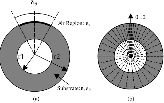
The principal steps in developing the MoL or PMoL algorithm are always the same, regardless the coordinate system. Therefore, the following mathematical steps are greatly abbreviated and we focus only on the aspects pertaining to the PMOL in cylindrical coordinates. Figure 1(a) shows the structure model of a cylindrical microstrip. A metal wall is placed at radiusR =r1, which is covered with a dielectric

substrate. The dielectric substrate has a depth of d = r2 −r1 with

dielectric constantεr. The width of the infinitely long microstrip line is denoted asw=r2δθ, whereδθ is the angular extent of the strip defined in the figure; the curvature coefficient, c, is introduced as the ratio

δ

Air Region: ε0

r1 r2

Substrate:

(a)

θ=0

(b) θ

εrε0

of inner radius r1 to outer radius r2, namely, c =r1/r2. Figure 1(b)

shows an example of PS discrete nodes distribution with the total lines

N = 40, the nodes quadratically cluster near θ= 0. It is obvious that with the same total lines, this one has more lines assigned metal strip than the MoL that uses equi-spaced discretizing. Under the cylindrical coordinate system, with the time harmonic dependence exp(jωt) being omitted for brevity, the field componentsEandHsatisfy the following equations:

Eθ= 1

k2−_β2

−jβ R

∂Ez

∂θ +jωµ ∂Hz

∂R

Hθ= 1

k2_−β2

−jβ R

∂Hz

∂θ −jωε ∂Ez

∂R

(1)

Thezdirection componentsEzandHzsatisfy the Helmholtz equation: 1

R ∂ ∂R

R∂φ

eh

∂R

+ ∂

2_φeh

R2_∂θ2 +

k2−β2φeh = 0 (2) whereφdenotes Ez orHz. Note that hereφ can be expressed as

φ=φeh(R, θ) exp(−jβz) whereβ is the phase constant.

Now the boundary conditions are needed to be properly selected. Thinking of the structure’s symmetry, just half of the structure in Figure 1(a) is adopted to simplify the original problem. Here the periodical boundary condition is given up and Neumann-Dirichlet boundary (ND) forEz and Dirichlet-Neumann boundary (DN) forHz are adopted. In fact, when the microstrip operates with fundamental mode, this half structure can be truncated into a smaller one for the fact that the higher the frequency is, the more the electromagnetic wave’s energy stays under the upper metal strip. From experience, when the truncated angular θN > (5−8)δθ, the error in the high frequency analysis introduced by truncated is negligible.

approximated by

f_θ(θi) = N

j=1

bijf(θj) for i= 1,2, . . . , N (3)

where N is the number of grid points and bij are the weighting co-efficients. To determine the weighting coefficients, bij, pseudospectral method assumes thatf(θ) is approximated by a high-order polynomial,

f(θ) = N

k=1

ckθk−1 (4)

Then, under the analysis of a linear polynomial vector space, the following explicit formulation is used to computebij:

bij =

M(1)_(θ

i) (θi−θj)M(1)(θj)

for j =i (5a)

bij = − N

j=1, j=i

bij (5b)

where

M(1)(θk) = N j=1,j=k

(θk−θj) (6)

In the above discussion, the sample points are arbitrary distribution in interval [0, θN]. In the pseudospectral method, each dependent variable in the differential problem is approximated by a polynomial of finite degree. The discrete approximating equations are then obtained by setting residuals to zero at an appropriate set of collocation points in the solution domain. The proper choice of collocation points is crucial in terms of accuracy, stability, and ease of implementation of boundary conditions. Usually, the equi-spaced node distribution is adopted but the large deviation is observed near the two endpoints in the pseudospectral method. The easiest way to offset these errors is to concentrate the nodes toward the ends of the interval. It is well known that the Chebyshev-distribution has smallest error and minimum node spacing, which decreases as

of boundary conditions are either Dirichlet-Neumann or Neumann-Dirichlet. The difference matrix with the DN lateral boundary condition is denoted by [aDN] and can be obtained as follows:

aDN_i,j =bi+1,j+1−bi+1,N+1

bN+1,j+1 bN+1,N+1

i= 1,2, . . . , N−1, j = 1,2, . . . , N−1 (7)

and the [aN D] forND lateral boundary condition is as follows:

aN D_i,j =bi+1,j+1−bi+1,1 b1,j+1

b1,1

i= 1,2, . . . , N −1, j= 1,2, . . . , N −1

(8)

For the first derivative ofEzwith respect to theθ-direction, one obtains

dEz

dθ = [aN D]Ez (9)

where Ez denotes the discretized Ez. Since Ez and Hz have dual boundary conditions, the finite difference expression for the first derivative of Hz becomes

dHz

dθ = [aDN]Hz (10)

Combining (9) and (10), one obtains for the second-order derivatives

d2Ez

dθ2 = [aDN] dEz

dθ = [aDN][aN D]Ez (11) d2Hz

dθ2 = [aN D] dHz

dθ = [aN D][aDN]Hz (12)

For a homogeneous layer, the second order pseudospectral difference operators De, h_θθ are the products of two different first order operators and their eigenvalues −λ2_e,h and the eigenvector matrices Te,h are defined as follows:

Dh_θθ Th

= [aN D] [aDN]

Th

=

Th λ2_h (13) [De_θθ] [Te] = [aDN] [aN D] [Te] = [Te]

real matrices there exist the real matrices Te,hsuch that

Te,h

₋1

D_θθe,h Te,h

=−diagd2_θθn (15a)

Th−1[aN D] [Te] =diag[dθθn] [Te]−1[aDN]

Th=−diag[dθθn]

(15b)

wherediag denotes a diagonal matrix;This directly solved from the Equation (13) and the [Te_{] is derived as follows [17]:}

[Te] = [aDN]

Th

diagd−_θθn1 (16) Along θ direction we perform a discretization by using N radial lines distributed as Chebyshev extreme nodes, as shown in Figure 1(b); it is:

θk =

θN 2

1 + cos(k−1)π

N−1

, k= 1,2, . . . , N (17)

where θN is truncated angular. Then differentials with respect to θ are taken place with differences; a set of coupled ordinary differential equations is obtained.

1

R ∂ ∂R

R∂Φ

e,h

∂R

+k2−β2−De,h_θθ Φe,h= 0 (18)

where Φe,h denoteEz orHz;

D_θθe,h

are the second-order differential’s discrete matrices ofEz orHz; and the first-order differential’s discrete matrices of Ez and Hz are

D_θe,h

. A transformed potential vectorU

is now introduced,

Ue,h=

Te,h

₋1

Φe,h (19)

then a set of decoupled ordinary equations with following forms can be got

1

R ∂ ∂R

R∂U

e,h i

∂R

+

k2−β2−d 2

θθi

R2

Ue,h_i = 0 (20)

where −d2_θθi is the ith eigenvalue of the second-order matrix

D_θθe,h

.

PMOL. WhereUe,h_i is the ith element in the vectorUe,h _{and U}e,h _is the transformation of the discrete z-direction components Ez orHz.

Equation (20) is the one-dimensional Helmholtz equation corresponding to the Bessel functions, whose common resolutions can be written as:

U_ieh(R) =

Aeh_1iJµi(Kc1R) +A₂eh_iNµi(Kc1R) r1 < R < r2 Aeh_3iKµi(Kc2R) R > r2

(21)

Kc1 =

K2

1 −β2 Kc2 =

β2−_K2 2

where µi = dθθi and Aeh1i, Aeh2i, Aeh3i are coefficients to be determined; J, N, K are Bessel, Neumann, and modified Bessel functions, respectively. In region 2, we omit the first modified Bessel function I because it does not satisfy the fields boundary conditions in the infinity.

Now we give the details of the derivation of the Green’s admittance matrix in the transformation domain. For tangential fields at R=r1,

i.e.,

Ez_R=r

1 = 0

∂Hz

∂R

R=r1

= 0

Ezi=

Be_[GJ

µi(Kc1R) +Nµi(Kc1R)] Ce[Kµi(Kc2R)]

Hzi=

Bh_[DJ

µi(Kc1R) +Nµi(Kc1R)] Ch_[K

µi(Kc2R)]

(22)

the “−” above the vector denotes in the transformation domain. Where

G=−Nµi(Kc1r1)

Jµi(Kc1r1)

D=−N

µi(Kc1r1) J_µi (Kc1r1)

then atR=r2

∂Ez1 ∂R

R=r2

=

Kc1

GJ_µi (Kc1r2) +Nµi (Kc1r2)

GJµi(Kc1r2) +Nµi(Kc1r2)

Ez1=P Ez1

∂Hz1 ∂R

R=r2

=

Kc1

DJ_µi (Kc1r2) +Nµi (Kc1r2)

DJµi(Kc1r2) +Nµi(Kc1r2)

Hz1 =QHz1

and

∂Ez2 ∂R

R=r2

= Kc2K

µi(Kc2r2) Kµi(Kc2r2)

Ez2 =T Ez2 ∂Hz2

∂R

R=r2

=T Hz2

(23b)

with the transformation

Eθ =

Th

₋1

Eθ Hθ = [Te]−1Hθ

Jθ = [Te]−1Jθ Jz =

Th

₋1 Jz

(24)

continuity boundary atR=r2 is

Ez1=Ez2

Hz1−Hz2

=−Jθ

Eθ1=Eθ2 Hθ1−Hθ2 =J z

(25)

From (1), we can get

      

Eθ1 =

1

Kc2₁

−jβ R2

ξEz1+jωµQHz1

Hθ1=

1 Kc2 1 jβ R2

ξHz1−jωε1P Ez1

(26a)       

Eθ2 =−

1 Kc2 2 −jβ R2

ξEz2+jωµT Hz2

Hθ2=−

1 Kc2 2 jβ R2

ξHz2−jωεT Ez2

(26b)

whereξ =µi, after some operations, we can get the following equation:

Jθi Jzi =

G11 G12 G21 G22

Eθi

Ezi

(27)

where

G11=

1

jωµ

Kc2₁ Q +

Kc2₂ T

G12= β ωµr2 ξ 1 Q− 1 T

G21=G12 G22= − β2_ξ2 r₂2jωµ

1

Kc2₁Q+

1

Kc2₂T

−

εrP

Kc2₁ + T Kc2₁

Qand T are defined in equation (23). So we can find

Eθi

Ezi

=Z Jθi Jzi

(28)

After transforming back to the spatial domain and taking into account that the tangential electric field vanishes on the metallic strip, a reduced matrix equation is obtained:

[Z]red

Jθi

Jzi

red =

Eθi

Ezi

red

= 0 (29)

The propagation constants or effective dielectric constant can be found form the corresponding determinantal equation:

DET|Z(β)|_red= 0 (30) It is a real equation to find a real root.

3. NUMERICAL RESULTS

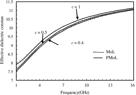
The effective dielectric constants for several structures are computed by using MoL and PMoL respectively. Figure 2 reveals how the curved surface affects the effective dielectric constant; the parameters are

7 7.5 8 8.5 9 9.5 10 10.5 11 11.5

1 4 7 10 13 16

Frequency(GHz)

E

ff

ect

iv

e d

iel

ect

ri

c con

st

an

c= 1

c= 0.5

c= 0.4

MoL PMoL

Figure 2. The effective dielectric constant results versus the operation frequency of a cylindrical microstrip with different curvature coefficient using MoL and PMoL. The parameters areεr= 11.7,d= 0.317 cm and

εr = 11.7, d = 0.317 cm and w/d= 1. The analysis region is limited in 0< θ <5δθ and total line numberN alongθdirection is 35 in MoL and 15 in PMoL.

Note that the difference for effective dielectric constant at low frequencies between the two methods is a little bigger; but from reference [18], we can find that these data are all in the error ranges.

9.6 9.8 10 10.2 10.4 10.6 10.8

10 15 20 25 30 35 40

Total Lines

E

ff

ect

iv

e

d

ie

lect

ri

c co

n

st

a

n

MoL

PMoL

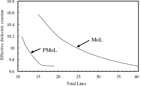
Figure 3. Convergence of the PMoL and MoL with frequency 6.5 GHz and c= 0.5.

The convergence curves are given in Figure 3. The operation frequency is 6.5 GHz; the structure parameter is the same as shown in Figure 1(a); and c= 0.5. It can be found that the pseudospectral MoL has much faster convergence rate than the conventional MoL. The new developed pseudospectral MoL adopts high-order interpolation polynomial to approximate the derivatives in controlling equation. As a result, it can approximate the smooth field inside the domain of interest so that the solution not only is analytical along line direction but also maintains high accuracy in discrete direction. Although the second-order differential matrix for the pseudospectral MoL is not sparse as that in conventional second-order MoL, the eigenvalues, eigenvectors and transformation matrix can be numerically solved by matured algorithm and the computation cost is little because of fewer lines needed in the numerical simulation.

4. CONCLUSIONS

demonstrate the efficiency and accuracy of this method. It can be seen that the pseudospectral MoL has a much faster convergence speed and it can achieve high accuracy in both analytical and discretized direction.

REFERENCES

1. Chang, H.-W. and M.-H. Sheng, “Field analysis of dielectric waveguide devices based on coupled transverse-mode integral equation — mathematical and numerical formulations,”Progress In Electromagnetics Research, PIER 78, 329–347, 2008.

2. Singh, V., Y. K. Prajapati, and J. P. Saini, “Modal analysis and dispersion curves of a new unconventional bragg waveguide using a very simple method,” Progress In Electromagnetics Research, PIER 64, 191–204, 2006.

3. Hernandez-Lopez, M. A. and M. Quintillan-Gonzalez, “A finite element method code to analyse waveguide dispersion,” J. of Electromagn. Waves and Appl., Vol. 21, No. 3, 397–408, 2007. 4. Zhou, X. and G. W. Pan, “Application of physical spline finite

element method (PSFEM) to fullwave analysis of waveguides,”

Progress In Electromagnetics Research, PIER 60, 19–41, 2006. 5. Tang, M. and J. F. Mao, “Transient analysis of lossy nonuniform

transmission lines using a time-step integration method,”Progress In Electromagnetics Research, PIER 69, 257–266, 2007.

6. Pregla, R. and W. Pascher, “The method of lines,” Numerical Techniques for Microwave and Millimeter-wave Passive Struc-tures, T. Itoh (ed.), 381–446, Wiley, New York, 1989.

7. Chen, R. S. and D. G. Fang, “Analysis of the open microstrip lines by method of lines,”International Journal of Microwave and Millimeter Wave CAD Engineering. Vol. 3, No. 2, 109–113, 1993. 8. Preglas, R., “MOL-BPM method of lines based beam propagation method,” Progress In Electromagnetics Research, PIER 11, 51– 102, 1995.

9. Pregla, R., “Higher order approximation for the difference operators in the method of lines,” IEEE Microwave and Guided Wave Lett., Vol. 5, No. 2, 53–55, Feb. 1995.

10. Helfert, S. F., “Applying oblique coordinates in the method of lines,”Progress In Electromagnetics Research, PIER 61, 271–278, 2006.

in cylindrical coordinates,” Microwave and Optical Technology Letters, Vol. 1, No. 5, 173–175, July 1988.

12. Chen, R. S., D. G. Fang, and X. G. Li, “Analysis of open microstrip lines by MOL,” International Journal of Microwave and Millimeter-wave Computer-aided Engineering, Vol. 3, No. 2, 109–113, 1993

13. Xiao, S., et al., “Analysis of cylindrical transmission lines with the method of lines,”IEEE Trans. Microwave Theory Tech., Vol. 44, No. 7, 993–999, July 1996.

14. Fornberg, B., A Practical Guide to Pseudospectral Methods, Cambridge University Press, 1996.

15. Chen, R. S., E. K. N. Yung, K. Wu, and Y. F. Han, “The generalized method of lines based on discretisation technique of pseudospectral method,” Microwave and Optical Technology Letters, Vol. 20, No. 5, 249–254, 1999.

16. Chen, R. S., D. X. Wang, and E. K. N. Yung, K. Wu, “Analysis of three-dimensional MMIC by spectral-pseudospectral domain technique,” Microwave and Optical Technology Letters, Vol. 31, No. 5, Dec. 5, 2001.

17. Chen, R. S., Z. H. Fan, E. K. N. Yung, and C. H. Chan, “Hybrid mode analysis of microstrip lines by the method of lines with pseudospectral discretization,”Microwave and Optical Technology Letters, Vol. 35, No. 3, 224–227, 2002.

18. Sarkar, T., “Finite difference frequency-domain treatment of open transmission structures,” IEEE Trans. Microwave Theory Tech., Vol. 38, 1609–1616, 1990.