SLL reduction in Antenna array using modified PSOGSA algorithm

(1)

International Journal of Research (IJR)

e-ISSN: 2348-6848, p- ISSN: 2348-795X Volume 2, Issue 08, August 2015

Available at http://internationaljournalofresearch.org

SLL reduction in Antenna array using modified

PSOGSA algorithm

1_{Gurjot Singh &}2_{Er. Mandeep Singh}

1_{Student, M.Tech, Department of Electronics and Communication, Punjabi University,}

Patiala, Punjab, India EMAIL:[email protected]

2_{Assistant Professor, Department of Electronics and Communication, Punjabi University,}

Patiala, Punjab, India

EMAIL: [email protected]

Abstract

In this work, we used a new hybrid population-based algorithm (PSOGSA) which is a combination of Particle Swarm Optimization (PSO) and Gravitational Search Algorithm (GSA). It can be used to improve the side lobe level of a linear array of antennas for use in personal communication devices in order to satisfy the situation of huge demand and compressed development cycle for antenna design. Using PSOGSA we can optimize the spacing between the elements of the linear array to produce a radiation pattern with minimum side lobe level and null placement control

1.1Introduction

The concept of an antenna array was first presented in military applications in the 1940s. This growth was significant in wireless communications as it enhanced the reception and transmission patterns of antennas used in these schemes. The array also enabled the antenna scheme to be electronically steered to receive or transmit information mainly from a specific direction without automatically moving the structure. As the field of signal processing developed, arrays could be used to receive energy (or information) from a specific direction while refusing information or nulling out the energy in unwanted guidelines. Consequently, arrays could be used to mitigate intentional interference (jamming) or unintentional interference (radiation from additional sources not meant for the scheme in question) directed toward the communication system. [1]

An antenna is a transducer to transform from a high frequency electric current to radio waves and vice versa. An antenna is used to transmit and receive radio waves. In transmission, a radio transmitter deliveries an oscillating radio frequency electric current to the antenna's terminuses, and the antenna emits the energy from the current as electromagnetic waves (radio waves). [2]

1.2 Antenna array

An antenna Array is a configuration of individual radiating components that are organized in space and can be used to yield a directional radiation pattern. Single-element antennas have radiation patterns that are wide and hence have a low directivity that is not appropriate for long distance communications. A high directivity can be still be attained with single-element antennas by increasing the electrical sizes (in terms of wavelength) and hence the physical size of the antenna. Antenna arrays come in numerous geometrical shapes, the most common being; linear arrays (1D). Arrays generally employ identical antenna elements. The radiating pattern of the array depends on the shape, the distance among the elements, the amplitude and phase excitation of the elements, and also the radiation pattern of discrete elements. [3]

The location of the nth antenna element is labelled by the vector𝑑_𝑛, where

(2)

International Journal of Research (IJR)

1.3Types of Antenna Arrays

1.3.1 Active and Passive array

An active array is one in which an active element (oscillator, amplifier, or mixer) is connected to the path of each radiator. These elements, along with the radiator, form the array module. Active antenna arrays are categorized as receiving, transmitting, and transceiving. Active antenna array advantages include the capability to increase radiated power, decrease thermal losses, increase reliability, and reduce the length of the paths between radiators and transceiving circuits.[4]

A passive array is one in which all elements are excited from a common oscillator or connected to a common receiver. Therefore, an immutable part of a passive array is the feed network connecting the elements. Passive antenna arrays are categorized as receiving, transmitting, and transceiving. They are finding wide use in variable purpose radars.

1.3.2 Linear Array

A linear array is one consisting of a group of identical elements placed in one dimension along a given direction. Linear arrays may have equidistant or non-equidistant element spacing’s. They are used in the analysis of the directional properties of arrays in antenna theory, and as building blocks for forming an array of arrays.[5]

1.3.3 Planar Array

A planar array has all elements located in a single plane occupying a definite area. Planar arrays have different configurations of elements. Rectangular triangular, or hexagonal, in which the elements are positioned at the vertices of the rectangles, right triangles, regular hexagons and also at the center of the hexagon.

1.3.4 Adaptive array

An adaptive array consists of an N-element array (usually in the receiving mode), where the useful signal is maximized based on an analysis of the signal to interference ratio. An important

aspect of adaptive arrays is the appropriate choice of weighting coefficients 𝑊(𝑡), which are placed between the antenna elements and a combining network. In the general case, the vector 𝑊(𝑡) must have the capability of changing the amplitude and phase of the received signal from each element.[6]

1.3.4 Cylindrical Array

A cylindrical array is one whose radiators are positioned on a cylindrical surface. The radiators used are wire and slot dipoles, open ended waveguides and horns, and spiral and dielectric rod antennas.

1.3.5Multi-beam Array

A multi-beam array supports the generation of several beams that can be used simultaneously for surveillance of a given sector. Each beam has its corresponding separate input channel. The basic element supporting generation of several beams is the multiple beam forming network.

1.4Modified Particle Swarm Optimization Algorithm

Particle Swarm Optimization (PSO) is a population based stochastic optimization tool inspired by social behavior of bird flock, fish school etc. as developed by Kennedy and Eberhart in 1995. In PSO, a member in the swarm, called a particle, represents a potential solution, which is a point in the search space. The global optimum is regarded as the location of food. Each particle has a fitness value and a velocity to adjust its flying direction according to the best experiences of the swarm in search for the global optimum in the D-dimensional solution space. The steps involved in modified PSO are given below:[6]

Step 1:

(3)

International Journal of Research (IJR)

Step 2:

Evaluate the fitness value of all particles.

Step 3:

Compare the personal best (𝑝_{𝑏𝑒𝑠𝑡}) of every particle with its current fitness value. If the current fitness value is better, then assign the current fitness value to 𝑝_{𝑏𝑒𝑠𝑡} and assign the current coordinates to 𝑝_{𝑏𝑒𝑠𝑡} coordinates.

Step 4:

Determine the current best fitness value in the whole population and its coordinates. If the current best fitness value is better than global best (𝑔_{𝑏𝑒𝑠𝑡}), then assign the current best fitness value to 𝑔_{𝑏𝑒𝑠𝑡}and assign the current coordinates to 𝑔_{𝑏𝑒𝑠𝑡} coordinates.[5]

Step 5:

Update velocity (𝑉_𝑖𝑑) and position (𝑋_𝑖𝑑) of the d-th dimension of the 𝑖 − 𝑡ℎ particle using the following equations:

𝑉_𝑖𝑑𝑡 = 𝜔 𝑡 ∗ 𝑉_𝑖𝑑𝑡−1 + 𝑐₁ 𝑡 ∗ 𝑟𝑎𝑛𝑑1_𝑖𝑑𝑡

∗ (𝑝𝑏𝑒𝑠𝑡_𝑖𝑑𝑡−1− 𝑋_𝑖𝑑𝑡−1+ 𝑐₂ 𝑡 ∗ 1 − 𝑟𝑎𝑛𝑑1_𝑖𝑑𝑡 ∗ (𝑔𝑏𝑒𝑠𝑡_𝑑𝑡−1 − 𝑋_𝑖𝑑𝑡−1)

𝑉_𝑖𝑑𝑡 > 𝑉𝑚𝑎𝑥𝑑 𝑜𝑟𝑉𝑖𝑑𝑡 < 𝑉𝑚𝑖𝑛𝑑 , 𝑡ℎ𝑒𝑛𝑉𝑖𝑑𝑡

= 𝑈(𝑉_𝑚𝑖𝑛𝑑 , 𝑈_𝑚𝑎𝑥𝑑 ₎

𝑋_𝑖𝑑𝑡 = 𝑟𝑎𝑛𝑑2_𝑖𝑑𝑡 ∗ 𝑋_𝑖𝑑𝑡−1+ 1 − 𝑟𝑎𝑛𝑑2_𝑖𝑑𝑡 ∗ 𝑉_𝑖𝑑𝑡

𝑐₁(𝑡), 𝑐₂(𝑡) = time-varying acceleration coefficients with 𝑐₁(𝑡) decreasing linearly from 2.5 to 0.5 and 𝑐₂(𝑡) increasing linearly from 0.5 to 2.5 over the full range of the search, and 𝑤(𝑡)

= time-varying inertia weight changing randomly between U(0:4 ; 0:9) with iterations,

𝑟𝑎𝑛𝑑₁, 𝑟𝑎𝑛𝑑₂ are uniform random numbers between 0 and 1, having different values in different dimension, t is the current generation number.

The above equation has been introduced to clamp the velocity along each dimension to uniformly distributed random value between

𝑉_𝑚𝑖𝑛𝑑 and 𝑉𝑚𝑎𝑥𝑑 if they try to cross the desired

domain of interest. These clipping techniques are sometimes necessary to prevent particles from explosion. The maximum velocity is set to the upper limit of the dynamic range of the search (𝑉𝑚𝑎𝑥𝑑 = 𝑋𝑚𝑎𝑥𝑑 ) and the minimum velocity (𝑉_𝑚𝑖𝑛𝑑 ) is set to (𝑋_𝑚𝑖𝑛𝑑 ).[7]

However, position-clipping technique is avoided in modified PSO algorithm. Moreover, the fitness function evaluations of errant particles (positions outside the domain of interest) are skipped to improve the speed of the algorithm.[5]

Step 6:

Repeat Steps 2 to 5 until a stop criterion is satisfied or a pre-specified number of iteration is completed, usually when there is no further update of best fitness value.[8]

1.6 Use of PSOGSA in SLL Reduction

Consider a linear antenna array, with 2N isotropic radiators placed symmetrically along the x-axis. The array factor in the azimuth plane can be written as,

AF 𝜙 = 2 . 𝐼_𝑛cos 𝑘. 𝑥_𝑛. cos 𝜙 + 𝜑_𝑛

𝑁

𝑛=1

Where𝑘 is the wave number, and 𝐼𝑛 , 𝜑𝑛 ,and 𝑥𝑛 are, respectively excitation magnitude, phase and location of the n-th element. If we further assume a uniform excitation of amplitude and phase (that is 𝐼𝑛= 1 and 𝜑𝑛 = 0) for all elements), the array factor can be further simplified as: [9]

AF 𝜙 = 2 . 𝐼𝑛cos 𝑘. 𝑥𝑛. cos 𝜙 𝑁

𝑛=1

(4)

International Journal of Research (IJR)

For side lobe suppression, the fitness function used is:

F = 1

∆𝜙_𝑖 𝐴𝐹 𝜙

2_𝑑𝜙 𝜙𝑢𝑖

𝜙𝑙𝑖

𝑖

To minimize both of them we use the above fitness function as and apply PSOGSA to it.

1.7 Results

Before simulations IWO, GA, TSA, MA, PSO and PSOGSA have several parameters which should be initialized. These parameters have been given below. [10]

For PSO we use the following settings:

 Swarm size = 30,

 𝑐₁ = 2, 𝑐₂ = 2,

 𝑤 is decreased linearly from 0.9 to 0.2,

 maximum iteration = 1000, and

 Stopping criteria = maximum iteration.

For PSOGSA we use the following settings:

 Population size = 30,

 𝑐₁′ _{= 0.5, 𝑐}

2′ = 1.5,

 w is any random number in [0, 1],

 Gravitational constant, G0 = 1,

 α = 20,

 maximum iteration = 1000, and

 Stopping criteria = maximum iteration.

For IWO we use the following settings:

 𝑠𝑑_𝑚𝑎𝑥 = 0.1, 𝑠𝑑_𝑚𝑖𝑛 = 10-5,

 initial number of plants = 30,

 maximum number of seeds = 5

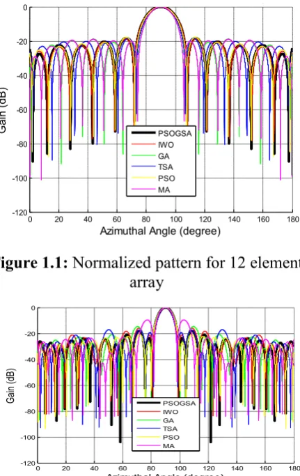
For rest of the competitor algorithms, we used the best possible parametric setup as explained in their respective literatures. All simulation results have been plotted as the Gain versus Azimuth Angle plot.[11]

Figure 1.1: Normalized pattern for 12 element array

Conclusion

All the simulation results show the array pattern from the PSOGSA algorithm using different number of array elements compared with that of the afore mentioned algorithms.

0 20 40 60 80 100 120 140 160 180

-120 -100 -80 -60 -40 -20 0

Azimuthal Angle (degree)

Gain (dB)

Normalized patterns for 12 element array.

PSOGSA IWO GA TSA PSO MA

0 20 40 60 80 100 120 140 160 180

-120 -100 -80 -60 -40 -20 0

Gain (dB)

PSOGSA IWO GA TSA PSO MA

0 20 40 60 80 100 120 140 160 180

-140 -120 -100 -80 -60 -40 -20 0

Gain (dB)

(5)

International Journal of Research (IJR)

From the results it is clear that PSOGSA has minimized SLL to the greatest extent and has a low gain value at the null directions as well. Thus, we can say that PSOGSA has successfully minimized both the sidelobe level and the required null directions. Therefore, we can use PSOGSA algorithm in the synthesis of linear array geometry for the purpose of suppressing side lobes and null placement in certain directions. PSOGSA can be used successfully to optimize the locations of array elements to exhibit an array pattern with either suppressed side-lobes, null placement in certain directions

References

[1] M. G. Bray, D. H. Werner, D. W. Boeringer and D. W. Machuga, “Optimization of thinned aperiodic linear phased arrays using genetic algorithms to reduce grating lobes during scanning,” Antennas and Propagation, IEEE Transactions on, vol. 50, no. 12, pp. 1732-1742, 2002.

[2] S. Caorsi, A. Lommi, A. Massa and M. Pastorino, “Peak sidelobe level reduction with a hybrid approach based on GAs and difference sets,” Antennas and Propagation, IEEE Transactions on, vol. 52, no. 4, pp. 1116-1121, 2004.

[3] M. I. Dessouky, H. A. Sharshar and Y. A. Albagory, “Efficient sidelobe reduction technique for small-sized concentric circular arrays,” Progress In Electromagnetics Research, vol. 65, pp. 187-200, 2006.

[4] L. J. Griffiths and C. W. Jim, “An alternative approach to linearly constrained adaptive beamforming,” Antennas and Propagation, IEEE Transactions on, vol. 30, no. 1, pp. 27-34, 1982.

[5] M. M. Khodier and C. G. Christodoulou, “Linear array geometry synthesis with minimum sidelobe level and null control using particle swarm optimization,” Antennas and Propagation, IEEE Transactions on, vol. 53,

no. 8, pp. 2674-2679, 2005.

[6] M. A. Panduro, D. H. Covarrubias, C. A. Brizuela and F. R. Marante, “A multi-objective approach in the linear antenna array design,”

AEU-International Journal of Electronics and Communications, vol. 59, no. 4, pp. 205-212, 2005.

[7] K.-K. Yan and Y. Lu, “Sidelobe reduction in array-pattern synthesis using genetic algorithm,” Antennas and Propagation, IEEE Transactions on, vol. 45, no. 7, pp. 1117-1122, 1997.

[8] C. Yu, “Sidelobe reduction of asymmetric linear array by spacing perturbation,”

Electronics Letters, vol. 33, no. 9, pp. 730-732, 1997.

[9] G. K. Mahanti, N. N. Pathak and P. K. Mahanti, “Synthesis of thinned linear antenna arrays with fixed sidelobe level using real-coded genetic algorithm,” Progress In Electromagnetics Research, vol. 75, pp. 319-328, 2007.

[10] D. G. Kurup, M. Himdi and A. Rydberg, “Synthesis of uniform amplitude unequally spaced antenna arrays using the differential evolution algorithm,” Antennas and Propagation, IEEE Transactions on, vol. 51, no. 9, pp. 2210-2217, 2003.