Volume 2007, Article ID 36871,13pages doi:10.1155/2007/36871
Research Article
Mobile Agent-Based Directed Diffusion in Wireless
Sensor Networks
Min Chen,1Taekyoung Kwon,2Yong Yuan,3Yanghee Choi,2and Victor C. M. Leung1
1Department of Electrical and Computer Engineering, University of British Columbia, Vancouver, BC, Canada V6T 1Z4 2School of Computer Science and Engineering, Seoul National University, Seoul 151-744, South Korea
3Department of Electronics and Information Engineering, Huazhong University of Science and Technology, Wuhan 430074, China
Received 29 November 2005; Revised 12 May 2006; Accepted 16 July 2006
Recommended by Deepa Kundur
In the environments where the source nodes are close to one another and generate a lot of sensory data traffic with redundancy, transmitting all sensory data by individual nodes not only wastes the scarce wireless bandwidth, but also consumes a lot of battery energy. Instead of each source node sending sensory data to its sink for aggregation (the so-called client/server computing), Qi et al. in 2003 proposed a mobile agent (MA)-based distributed sensor network (MADSN) for collaborative signal and information processing, which considerably reduces the sensory data traffic and query latency as well. However, MADSN is based on the assumption that the operation of mobile agent is only carried out within one hop in a clustering-based architecture. This paper considers MA in multihop environments and adopts directed diffusion (DD) to dispatch MA. The gradient in DD gives a hint to efficiently forward the MA among target sensors. The mobile agent paradigm in combination with the DD framework is dubbed mobile agent-based directed diffusion (MADD). With appropriate parameters set, extensive simulation shows that MADD exhibits better performance than original DD (in the client/server paradigm) in terms of packet delivery ratio, energy consumption, and end-to-end delivery latency.
Copyright © 2007 Min Chen et al. This is an open access article distributed under the Creative Commons Attribution License, which permits unrestricted use, distribution, and reproduction in any medium, provided the original work is properly cited.
1. INTRODUCTION
Recent years have witnessed a growing interest in deploying a sheer number of microsensors that collaborate in a dis-tributed manner on sensing, data gathering, and processing. In contrast with IP-based communication networks based on global addresses and routing metrics of hop counts, sensor nodes normally lack global addresses. Also, as being unat-tended after deployment, they are constrained in energy sup-ply (e.g., small battery capacity).
These characteristics of sensor networks require energy awareness at most layers of protocol stacks. To address such challenges, most of researches focus on prolonging the net-work lifetime, allowing scalability for a large number of sen-sor nodes, or supporting fault tolerance (e.g., sensen-sor’s failure and battery depletion) [2,3]. Most energy-efficient proposals are based on the traditional client/server computing model, where each sensor node sends its sensory data to a back-end processing center or a sink node. Because the link band-width of a wireless sensor network is typically much lower than that of a wired network, a sensor network’s data traffic
may exceed the network capacity. To solve the problem of the overwhelming data traffic, Qi et al. [1] proposed the mo-bile agent-based distributed sensor network (MADSN) for scalable and energy-efficient data aggregation (this aggrega-tion process is called collaborative signal and informaaggrega-tion processing in [1]). By transmitting the software code, called “mobile agent (MA)” to sensor nodes, the large amount of sensory data can be reduced or transformed into small data by eliminating the redundancy. For example, the sen-sory data of two closely located sensors are likely to have re-dundant or common part when the data of two sensors are merged. Therefore, data aggregation is a necessary function in densely populated sensor networks in order to reduce the
sensory data traffic. However, MADSN operates based on the
Segment ROI (region of interest)
2
Collect reduced data
3
Migrate to sink node 1 Migrate to target region
Figure1: Mobile agent-based image sensor querying.
network architecture, which may be suitable for a wide range of sensor applications. Thus, we will consider MA in multi-hop environments with the absence of a clusterhead. With-out clusterhead, we have to answer the following questions. (1) How is an MA routed from sink to source, from source to source, and from source to sink in an efficient way? (2) How does an MA decide a sequence to visit multiple source nodes? (3) If the sensory data of all the source nodes cannot be fused into a single data packet with a fixed size, will the MA paradigm still perform more efficiently than the client/server computing model? How about in the environments where the source nodes are not close to one another, and the sen-sory data do not have enough redundancy?
With the development of WSN, “one-deployment mul-tiple applications” is a trend due to the application-specific nature of sensor networks. Such a trend must require sensor nodes to have various capabilities to handle multiple appli-cations, which is economically infeasible. In general, using memory-constrained embedded sensors to store every possi-ble application in their local memory is impossipossi-ble. Thus, a way of dynamically deploying a new application is needed.
To have an in-depth look at problems we mentioned above and why the MA is necessary, we investigate the fol-lowing scenario of an image recognition application in
wire-less sensor networks. InFigure 1, we assume that a number
of image sensors are deployed to monitor a remote region. Transmitting the whole pictures taken by individual sensors to a sink node may be overwhelming for the wireless link, or even unnecessary in the case that the sink node needs only the region of interest (ROI) of the picture (e.g., human face or vehicle identification number plate). Thus, instead of transmitting the whole picture, a source node extracts the ROI from the whole picture using an image segmentation algorithm. However, a single kind of image segmentation al-gorithm cannot achieve fairly good performance for all kinds of images to be extracted. For example, a code for ing a face image will be different from the one for segment-ing a vehicle identification number plate. However, a sensor network may require various image processing algorithms to
handle different kinds of images of interest. It is impossible to keep all kinds of codes in a sensor node’s limited memory. In order to solve this problem, the sink node can dispatch an MA carrying a specific image segmentation code to the sensors of interest. Carrying a special processing code, the MA enables a source node to perform local processing on the sensed data as requested by the application. When the MA reaches and visits the sensors of interest, the image data at each target sensor node can be reduced into a smaller one by image-segment processing.
Since multiple hops may exist among target source nodes, the migration behavior of the MA becomes complicated and it is important to find out a way to dispatch the MA efficiently among the sensors of interest. Directed diffusion (DD) [4,5] is a prominent example of data-centric routing based on ap-plication layer context and local interactions. The gradient in DD gives a hint to efficiently forward the MA among tar-get sensors. The MA paradigm in combination with the DD
framework is dubbed mobile agent-based directed diffusion
(MADD). This paper investigates this combination: is it fea-sible to conduct DD with the mobile agent paradigm? How does MA operate in detail? In which condition does MADD outperform DD in terms of energy consumption and end-to-end delay?
This study also provides insights into the behavior of MA in multihop wireless environments, contributing to a better understanding of this novel combination of mo-bile agent paradigm and a holistic DD framework. Exten-sive simulation-based comparison between original DD and MADD shows that, depending on the parameters, MADD can significantly reduce the energy consumption and end-to-end delay. The rest of this paper is organized as follows.
Section 2presents related work. We describe MADD design
issues and algorithm in Sections3and4, respectively. Sim-ulation model and results are explained in Sections5and6, respectively. Finally,Section 7will conclude the paper.
2. RELATED WORK
Recently, mobile agents have been proposed for efficient data
dissemination in sensor networks [1, 6–12]. In a typical
client/server-based sensor network, the occurrence of cer-tain events will alert sensors to collect data and send them to a sink node. However, the introduction of a mobile agent (MA) leads to a new computing paradigm, which is in con-trast to the traditional client/server-based computing. The MA is a special kind of software which visits the network either periodically or on demand (when the application re-quires). It performs data processing autonomously while mi-grating from node to node. Although there are advantages and disadvantages (code caching, safety, and security) of us-ing MAs [3] in a particular scenario, their successful applica-tions range from e-commerce [6] to military situation aware-ness [7]. They are found to be particularly useful for data fu-sion tasks in distributed sensor networks. The motivations for using MAs in distributed sensor networks have been ex-tensively studied in [1].
for sensor networks. It provides the following mechanisms: (a) for a sink node to flood a query toward the sensors of interest (say, sensors detecting event), (b) for intermediate nodes to set up gradients to send data along the routes to-ward the sink node. DD provides high quality paths, but requires an initial flood of the query to explore paths. In DD, the publish/subscribe mechanism provides a sensor net-work with application context by attribute-based naming. Attribute-based naming specifies which sensors are respon-sible for responding queries, and how intermediate sensors perform in network processing. Attributes describe the data which a sink node desires, by specifying sensor types, desired data rate, and possibly some geographical region. A moni-toring node becomes a sink, creating attributes of interest specifying a particular kind of data. The interest is propa-gated over the network towards sensor nodes in the specified region. A key feature of DD is that every sensor node can be application-aware, which means that nodes store and in-terpret interests, rather than simply forwarding them along. Each sensor node that receives an interest maintains a table that contains which neighbor(s) sent that interest. To such a neighbor, it sets up a gradient. A gradient is used to evaluate the eligibility of a neighbor node as a next hop node for data dissemination. After setting up a gradient, the sensor node redistributes the interest by broadcasting the interest. As in-terests travel across the network, sensors that match inin-terests are triggered and the application activates its local sensors to begin collecting and sending data.
3. OVERVIEW OF THE MADD DESIGN
In this section, we discuss the key design issues of MADD. Be-fore describing them, we first present our assumptions about MADD and its applications.
(1) Compared with the distance to the sink node, the tar-get sensor nodes are geographically close to each other. (2) Only source nodes matching interest packets will store the processing code carried by an MA. The sink does not flood processing code to the whole network, since the associated communication overhead may be too high. For example, shipping a mobile agent with face detection code would incur an overhead of over 1 MB. However, most of the sensor nodes may not be queried by this application at all.
(3) Processing code is stored in the source node when the MA visits it at the first time. The processing code will be operating until the task is scheduled to finish. It may be discarded when the task is finished.
(4) The locally processed data in each source node will be aggregated into the accumulated data result of the MA by a certain aggregation ratio.
3.1. Application redundancy eliminating by MA-assisted local processing
As described in Section 1, due to the application-specific
nature of sensor networks, a sensor should have various capabilities to handle multiple applications. However, it is
unrealistic for a memory-constrained embedded sensor to store every possible application code in its local memory.
The introduction of MA not only provides an efficient way
of dynamically deploying a new application, but also allows a source node to perform local processing on the raw data as requested by the application. This capability enables a re-duction in the amount of data to be transmitted since only relevant information will be extracted and transmitted. Letr (0< r < 1) be the reduction ratio by the MA-assisted local processing, letSidatabe the size of raw data at sourcei, and let
Ribe the size of reduced data. Then,
Ri=Sidata·(1−r). (1)
3.2. Aggregation
The degree of sensed data correlation among sensors is closely related to the distance between sensors so that it is very likely for closely located sensors to generate redundant sensed data. Therefore, data aggregation, which eliminates unnecessary data transmissions, is a necessary function in densely populated sensor networks in order to refine the sensed data as well as to extend the network lifetime. Because the aggregation decisions are made as the data is dissemi-nated in the network, this is also referred to as in-network processing.
In DD, different data packets which are completely/ partially redundant each other are forwarded to the sink through multiple paths with a low probability to be aggre-gated. This aggregation technique can be considered as op-portunistic aggregation.
In contrast, the MA aggregates individual sensed data when it visits each target source. Though this kind of aggre-gation technique is typically used in clustering or aggreaggre-gation tree-based data dissemination protocols, the aggregation in MADD does not need any overhead to construct these special structures. Note that MADD builds the gradient for routing as DD does, and does not need more control overhead than DD.
We calculate the size of data result accumulated by the MA using the similar method in [9]. A sequence of data result can be fused with an aggregation ratio (ρ, 0 ≤ ρ ≤ 1). Let
Si
mabe the amount of accumulated data result after the MA
leaves sourcei, whereRi is the amount of data that will be aggregated byρ. Then,
S1 ma=R1,
S2
ma=R1+ (1−ρ)·R2
.. .
Si
ma=Si−ma1+ (1−ρ)·Ri
=R1+
i
k=2
(1−ρ)·Rk.
(2)
In (2), there is no data aggregation in the first source. The value ofρis dependent on the type of application. For the
im-age processing application described inSection 1, when we
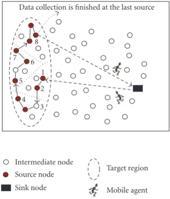
Data collection is finished at the last source
8 7
6 5
4 3 2 1
Intermediate node Source node Sink node
Target region Mobile agent
Figure2: Gradient-based solution for deciding the order of source nodes to be visited.
only if statistical characteristics of the image are known (e.g., Slepian-Wolf coding schemes [13]), which implies that data aggregation may not be achieved efficiently. By comparison, the application considered in [1] is an extreme example, where the sensory data can be fused into a data with fixed size (say,ρ=1).
3.3. Efficient routing
The order of source nodes to be visited by the MA can have a significant impact on energy consumption. Finding an op-timal source-visiting sequence is an NP-complete problem. In [10], a genetic algorithm-based solution to compute an approximate solution is presented. Though global optimiza-tion can be achieved using genetic algorithm, it is not a lightweight solution for sensor nodes that are constrained in energy supply. This paper adopts a gradient-based
solu-tion (inSection 4.3) for the MA to dynamically decide the
route.Figure 2gives an example of deciding source-visiting sequence through the gradient-based solution.
4. THE MADD ALGORITHM
Section 4.1gives an overview of the algorithm. Section 4.2
describes the structure of the MADD packet.Section 4.3 il-lustrates MADD with the details. Then, we give a simple per-formance analysis inSection 4.4
4.1. Algorithm overview
The flowchart of the MADD protocol is shown inFigure 3.
Once receiving a new task as requested by an application, the sink initially floods an interest packet to find out the sources which will perform the task. If the sources in the target re-gion receive the interest packets, they flood exploratory data
to the sink individually. Then, the sink will receive these ex-ploratory data packets from various sources and decide the list of sources that will be visited by an MA. In the list, there are two sources whose positions are important, namely, the first source which the MA will visit (FirstSrc) and the last source (LastSrc).
The MA-related operation begins at the point of the sink dispatching MA and ends when the MA returns to the sink with collected results. The whole route can be generally
di-vided into three parts demarcated by FirstSrc and LastSrc
(i.e., from the sink toFirstSrc, fromFirstSrctoLastSrc, and fromLastSrcto the sink).
In most cases, each source is expected to generate the sen-sory data periodically with some interval, which means the same code (MA) needs to be stored for multiple runnings. Thus, when the MA arrives at theFirstSrc, it will be stored. Then,FirstSrcsets aCreate-MA-Timer, which is used to trig-ger the next round to dispatch the MA to collect data from the relevant sources again. Obviously, the interval between the successive rounds will be equal to the sensory data gener-ating rate which is set to the value of theCreate-MA-Timer. This round will be repeated until the task is finished. A round can also be defined as the interval from the time that an MA collects the data packet in theFirstSrcto the time that it col-lects the data packet inLastSrc. At the end of the last round, the task is finished.
When theCreate-MA-Timerexpires,FirstSrcstarts a new round by dispatching the MA along all the sensors. After an MA visits theLastSrc, it discards the processing code and car-ries the aggregated result to the sink. The sink will be ex-pected to receive an MA by the desired data rate until the task is finished.
Based on the above illustration, the differences between MADD and client/server-based WSN can be listed as follows.
(1) All the relevant sources in client/server-based WSN send sensory data individually with a specified inter-val; while in MADD, a single MA visiting all the rele-vant sources will collect the data. The interval between reports to the sink is decided by the dispatching rate of the MA.
(2) In client/server-based WSN, data results are sent back in parallel from all sources, or return to the sink; while in MADD, data is collected by the MAs visiting all the target sensors along a single path.
4.2. Mobile agent packet format
The information contained in an MA packet is shown in
Figure 4. The pair ofSinkIDandMA SeqNumis used to
iden-tify an MA packet. Whenever a sink dispatches a new MA packet, it will increment theMA SeqNum.FirstSrcand Last-Srcare the source nodes scheduled to be visited firstly and lastly by the MA, respectively. The pair ofFirstSrcand
Last-Srcindicates the beginning and ending points of MA’s data
Idle state
A Receive new task(I am a sink) Flood interest
A Receive interset(I am a source) Flood exploratorydata (E-data)
B
ReceiveE-datas sent bynsources
(I am the sink)
Create MA
SetFirstSrc
andSrcList
to the MA
Dispatch MA
C Visited by MA(I amFirstSrc) Store the MA Create-MA-TimerStart No D
Expire Create-MA-Timer
(I amFirstSrc)
Create MA by copying the
stored one
Last round? Yes
E (I am non-Visited by MAFirstSrc) Am I thein theSrcListLastSrc? No MA collects data andmigrates toNextSrc
in theSrcList
Yes MA collects data and migrates to the sink
Figure3: Flowchart of the basic MADD protocol.
Fixed attributes
SinkID MASeqNum FirstSrc LastSrc RoundIdx LastRoundFlag
Variable attributes
NextSrc NextHop ToSinkFlag SrcList
Payload
Processing code Data
Figure4: MA packet structure.
of the whole task. The flag is set byFirstSrc. When an MA withLastRoundFlagset arrives at a source node, it can make the system unmount the corresponding processing code after its execution.
When an MA migrates, it may change variable attributes.
NextSrcspecifies the next destination source node to be
vis-ited.NextHopindicates the immediate next hop node which
is an intermediate sensor node or a target source node. If
NextHop is equal to NextSrc, it means that the next hop node is current destination source.SrcListcontains the iden-tifiers (IDs) of target sensor nodes that remain to be visited in the current round. It does not contain any information of source-visiting sequence sinceNextSrcis dynamically de-cided when an MA arrives at a source node (exceptLastSrc).
SrcListinitially contains all the IDs of source nodes when an MA is created. The corresponding ID will be deleted after the MA visits the source node. If all the target sources have been
visited by the MA,ToSinkFlagis set to indicate that the des-tination of the MA is the sink.NextSrc,NextHop,SrcList, and
ToSinkFlaghint the dynamical route of MA migration. Pay-load includes two kinds of data. One isProcessingCodewhich is used to process sensed data; the other isDatawhich carries the accumulated data result. The size ofDatais zero when an MA is generated, and increases while the MA migrates from source to source.
4.3. Detailed illustration of MADD protocol and gradient-based MA routing
A B C
D 14
15 13 12
16 17
11 10
9
8 7 6
5 4
1 2
3 E Sink
Sink node Intermediate node
Intermediate source node First source node Last source node
Positive reinforcement Mobile agent migrates toward event region Mobile agent migrates
among source nodes Mobile agent migrates
along reinforced path
Figure5: Second phase of MADD.
messages to adjust gradients in the case of network changes (due to node failure, energy depletion, or mobility), tempo-rary network partitions, or to recover from lost exploratory messages. The path reinforcement and the subsequent trans-mission of data along reinforced paths constitute the second phase of two-phase pull DD. The first phase of MADD is identical to that of DD, however, in addition to path rein-forcement, in the second phase, an MA is sent to target source nodes matching the sink’s interests.
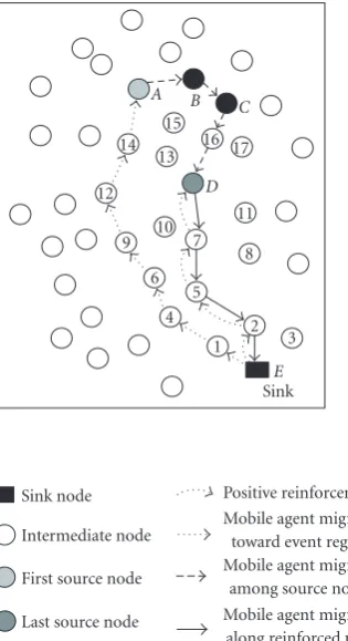
Figure 5 depicts the detailed operation of the second
phase in the MADD scheme. At the end of the first phase, the target sensor nodes generate multiple exploratory mes-sage flows to the sink. Since the ultimate goal is the detection of events in sensor networks [14], the sink may stop handling any exploratory message flows if it considers that the number of source nodes is large enough to meet the requirement of reliable event detection. Thus all the source nodes or only a subset of these nodes will be chosen to be visited by MA. Among the target source nodes to be visited, the sink will choose the first and last source nodes. Then, the sink
gen-erates an MA with the packet format described inFigure 4,
and dispatches it to the first source. At the same time, the sink reinforces the path to the last source. When the MA ar-rives at the first source node, it is stored in the node. We di-vide the whole task period into rounds, where each round requires the MA to visit all the chosen target sensors and to return the data result to the sink. The MA starts from the first
source (or from the sink only in the first round) and arrives at the last source. Finally, the MA will carry the data result to the sink along the reinforced path. In the first round, in addition to that the MA moves from source to source to col-lect and aggregate information, it also copies processing code into the memory of each source node. At the beginning of each round, the first source node will construct another MA from its memory and dispatch it to initiate the new round. Since processing code has already resided in each source node after the first round, the MA does not carry the processing code any more in the following rounds. When the whole task is finished, all the source nodes will discard the processing code.
In the first phase of MADD, the initial flooding of the interest enables each sensor node (e.g., intermediate sensor node or source node) to set up exploratory gradients [15] which are used to deliver exploratory messages intended for path setup and repair. The exploratory gradients, which are denoted as exp., are shown inFigure 6(a). After path
rein-forcement, the updated gradients are shown inFigure 6(b).
The gradient to deliver MA is denoted by MA. The identifier of each node is equal to the one inFigure 5.
In MADD, target source nodes flooding exploratory mes-sages enable sensor nodes to set upToSourceEntry, which is a kind of gradient toward each target source.ToSourceEntry
is used for MA to roam among source nodes. In this paper, a time-to-live (TTL) field is set in exploratory message to man-date only the sensor nodes within the target region to set up theirToSourceEntries. The value of TTLis decreased as ex-ploratory message is propagated hop by hop. If the value is
equal to 0, sensor nodes do not set up ToSourceEntryany
more. Among all the neighbors of a sensor node, only the neighbor who first relays the exploratory message of a spe-cific target source will be chosen as the sensor node’s Nex-tHopin theToSourceEntry. InFigure 5, nodesA,B,C, and
Dare the target source nodes. TheToSourceEntriesset up by nodesA,B,C, 16, andDare shown inFigure 7.
Based on the gradients andToSourceEntries, a migrating route is decided by the following three operating elements.
(1) ChooseFirstSrcandLastSrc. According to (2), the size of an MA is the minimum inFirstSrcwhile it becomes
the maximum inLastSrc. Thus, to reduce total
com-munication overhead,FirstSrcshould be the farthest target sensor from the sink, whileLastSrcshould be the closest one. In this paper, the target source which is the last (first) to send exploratory messages to the sink is chosen asFirstSrc(LastSrc). The sink will reinforce the path toLastSrc.
(2) Decide source-visiting sequence.Except thatFirstSrcand
LastSrcare chosen by the sink, the sequence of visiting the other source nodes is dynamically decided by each target sensor inSrcList. For example, when an MA ar-rives at nodeAinFigure 5, the node will choose the
closest next source node based on its ToSourceEntry
shown in the first row ofFigure 7. Since the lowest la-tency of nodeBis the least, it implies that nodeBis the closest source node from nodeAand is chosen as
Gradient (interest SeqNum = 1)
D Directiontype exp.7 exp.10 exp.13 exp.16 exp.17 exp.11
7 Direction 5 6 10 D 11 8
type exp. exp. exp. exp. exp. exp.
5 Direction 4 6 7 8 2 1
type exp. exp. exp. exp. exp. exp.
2 Direction E 1 5 3 — —
type exp. exp. exp. exp. — —
(a)
Gradient (interest SeqNum = 1)
D Directiontype MA7 exp.10 exp.13 exp.16 exp.17 exp.11
7 Directiontype MA5 exp.6 exp.10 exp.D exp.11 exp.8
5 Direction 4 6 7 8 2 1
type exp. exp. exp. exp. MA exp.
2 Direction E 1 5 3 — —
type MA exp. exp. exp. — —
(b)
Figure6: Gradients to the sink. (a) Before reinforcement. (b) After reinforcement.
ToSourceEntry(exploratory message SeqNum = 5)
Source A B C D
A Lowest Latency (ms)NextHop —— 4.B46 8B.24 1614.32
B Lowest Latency (ms)NextHop 4.A47 —— 4C.43 12C.89
C Lowest Latency (ms)NextHop 8.B16 4.B32 —— 816.52
16 NextHop 15 C C D
Lowest Latency (ms) 9.65 7.56 4.86 5.08
D Lowest Latency (ms)NextHop 1410.15 1216.67 816.73 ——
Figure7:ToSourceEntrysetup after exploratory messages flooding.
(3) Find the next hop node to route an MA along the entire path from sink to source, source to source, and source to sink.Dispatched by the sink, an MA migrates to
First-Src in the same manner as a reinforcement message
is forwarded in original DD. When the MA migrates among target sources, its next hop node will be de-cided according to current node’sToSourceEntry. The MA will return to the sink using the reinforced path (e.g., pathD-7-5-2-EinFigure 5).
4.4. Performance analysis
In this section, we present a simple analysis that evaluates the key performance metrics of DD and MADD, including the average end-to-end delay for a data packet delivery (Tete) and
the cumulative energy consumption involved in forwarding data packets from all the source nodes to the sink in one round(E).
LetTddandTmadenoteTeteof DD and MADD,
respec-tively. It accounts for all possible delays during data dissem-ination, caused by queuing, retransmission due to collision
at the MAC, and transmission time. Let H be the number
of hops along the path betweenLastSrcand the sink, which
is actually the lowest latency path among all the source-sink
pairs. Let H+hbe the average number of hops of all the
source-sink pairs in DD.Sdatais the size of sensed data andSh
is the size of packet header. Letvnbe the data rate at MAC layer; let tctrl be the total delay for control messages (say,
ACK) during a successful data transmission. In DD, multi-ple data results sent in parallel from all sources are likely to contend for the channel (CSMA-CA) and potentially collide, which causes additional delay for data retransmissions, espe-cially as the number of source nodes becomes large. Lettaccess
be the average latency to transmit a data packet successfully in DD. LetTrbe the average latency for path reinforcement. Letndatabe the number of data packets delivered to the sink
during the task. Then,Tddis equal to
Tdd=nTr data
+ S
data+Sh
vn +tctrl+taccess
·(H+h)
≈ S
data+Sh
vn +tctrl+taccess
·(H+h)
ifndata1
.
(3)
In MADD,Tma is the average time interval between the
time an MA is created and the time the MA returns to the sink. LetTpbe the delay of the MA migrating from the sink to theFirstSrc; letTroambe the average latency of MA roaming
from theFirstSrcto theLastSrc; letTbackbe the average delay
of MA migrating from theLastSrcto the sink.
Letτbe the MA accessing delay (e.g., the time for an MA to amount processing code in target source). Let Sp be the size of processing code; letvpbe the data processing rate; let
Si
ma be the size of MA at sourcei; let N be the number of
source nodes. Then,Troamis equal to
Troam=
N
i=1
τ+Sdata
vp +
Si
ma+Sp+Sh
vn +tctrl
. (4)
In (4),Simais equal to
Si
ma=Si−ma1+Sdata·
1−ri·1−pi. (5)
LetSNma be the size of an MA packet after the MA visits
LastSrc. Then,Tbackis equal to
Tback=
SN
ma+Sh
vn +tctrl
Then,Tmacan be calculated as follows:
Tma= nTp data
+Troam+Tback
≈Troam+Tback
ifndata1
.
(7)
LetEddandEmadenoteEof DD and MADD, respectively.
Letmtxandmrxbe the energy consumption for receiving and
transmitting a bit, respectively. Letbbe the fix energy cost to transmit a packet. Letectrlbe the energy consumption of
control messages exchanged for a successful data transmis-sion. Leteretx be the energy consumption of packet
retrans-missions for a successful data transmission in case of conges-tion in DD. Then,Eddis equal to
Edd=
Sdata+Sh·mtx+mrx
+b+ectrl+eretx
·(H+h)·N. (8)
In MADD, letEpbe the energy consumption of MA
mi-grating from the sink to theFirstSrc; let Eroam be the
aver-age energy consumption of MA roaming from theFirstSrc
to LastSrc; letEback be the average energy consumption of
MA migrating from theLastSrcto the sink. Letmpbe the en-ergy consumption for processing a bit. Then,Eroamis equal
to
Eroam=
N
i=1
Sdata·mp+Sima+Sp+Sh
·mtx+mrx
+b+tctrl
.
(9)
Ebackis equal to
Eback=
SN
ma+Sh
·mtx+mrx
+b+tctrl
·H. (10)
Finally,Emacan be calculated as follows:
Ema=nEp data
+Eroam+Eback
≈Eroam+Eback
ifndata1
.
(11)
5. THE SIMULATION MODEL
5.1. Simulation settings
In order to demonstrate the performance of MADD, we choose a client/server-based scheme (i.e., DD) to compare
with MADD. We use OPNET [16, 17] for discrete event
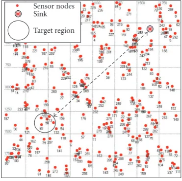
simulation.Figure 8illustrates our sensor network.Figure 9 shows the protocol stack of our sensor node model; it in-cludes application layer, routing layer, data link layer, and physical layer. Each task requires periodic transmission of data packets with a constant bit rate (CBR) of 1 packet/s. The sensor nodes are battery operated except the sink. The sink is assumed to have infinite energy supply. We assume that both the sink and sensor nodes are stationary. The sink is located close to one corner of the area, while the target sensor nodes are specified at the other corner. We use the energy model in [18]. The energy consumption parameters are shown in
Sensor nodes Sink Target region
Figure8: Sensor network model.
Sensor
App manager
MADD routing
Wlan mac intf
Wirless lan mac
Wlan port rx 0 Wlan port tx 0
Application layer
1.Sensor module: constant bit rate (CBR) real-time & best-effort traffic generator 2.App manager module:
application-specific in-network processing Routing layer
MADD and directed diffusion routing Data link layer
IEEE 802.11 implementation + interface
Physical layer
WLAN receiver (rx) + WLAN transmitter (tx)
Figure9: Sensor node model.
Table 1. Every node starts with the same initial energy bud-get (4,500 W·s) [18]. We use the following equation to cal-culate the energy consumption in three states (transmitting, receiving, or overhearing):
m×PacketSizeMAC+b+Pidle×t×1000 (μW·s). (12)
Note that to express power consumption in idle state,Pidle,
inμWunit, 1000 is multiplied. In (12),mrepresents the in-cremental cost compared to the power consumption in idle state,brepresents the fixed cost independent of the packet size,trepresents the duration of the state, andPacketSizeMAC
represents the size of the MAC packet.
Table1: Energy consumption parameters configuration of lucent IEEE802.11 WaveLAN card [17].
Normalized initial energy of sensor node (W·sec) 4500
Incremental cost (μW·s/bytes)
mtx 1.9
mrecv 0.5
moverhearing 0.39
btx 454
Fixed cost (μW·s) brecv 356
boverhearing 140
Pidle(mW) 843
Table2: Simulation setting.
Basic specification
Network size 500 m×500 m
Topology configuration mode Randomized Total sensor node number 1500 Data rate at MAC layer (vn) 1 Mbps
Transmission range of sensor node 60 m
Long retry limit Default: 4
Short retry limit Default: 7
Sensed traffic specification
Number of source nodes (N) Default: 5 Size of sensed data (Sdata) Default: 1 KB
Size of control message Default: 128 B Sensed data packet interval Default: 1 s
Duration Default: 300 s
MADD specification
Raw data reduction ratio (r) in (1) Default: 0.8 Aggregation ratio (ρ) in (2) Default: 0.2 MA accessing delay (τ) in (4) Default: 10 ms Data processing rate (vp) in (4) Default: 50 Mbps
Size of processing code (Sproc) Default: 2 MB
5.2. Performance metrics
In this section, five performance metrics are evaluated.
(i) Reliability (packet delivery ratio). It is denoted byP. It is the ratio of the number of data packets delivered to the sink to the number of packets generated by the source nodes.
(ii)Energy consumption per successful data delivery. It is denoted by e. It is the ratio of network energy con-sumption to the number of data packets successfully delivered to the sink. The network energy consump-tion includes all the energy consumpconsump-tion by transmit-ting and receiving during simulation. As in [1], we do not account energy consumption for idle state, since this part is approximately the same for all the schemes simulated. LetEtotalbe all the energy consumption by
transmitting, receiving, and overhearing during sim-ulation. Recall thatndata denotes the number of data
packets delivered to the sink. Then,eis equal to
e=Entotal
data.
(13)
(iii) Average end-to-end packet delay.It is denoted byTete.
And we also useTdd andTma to denote the average
end-to-end delays in DD and MADD, respectively. It includes all possible delays during data dissemination, caused by queuing, retransmission due to collision at the MAC, and transmission time.
(iv) Energy∗delay/reliability.In sensor networks, it is im-portant to consider both energy and delay. In [19], the combined energy∗delay metric can reflect both the en-ergy usage and the end-to-end delay. Furthermore, in unreliable environment, the reliability is also an im-portant metric. In this paper, we adopt the following metric to evaluate the integrated performance of relia-bility, energy, and delay:
η= e·Tete
P . (14)
6. PERFORMANCE EVALUATION
In this section, we compare the above performance met-rics of DD and MADD, and determine the conditions un-der which MADD is more efficient than DD by simulation. Though these conditions are affected by many parameters, only a set of important parameters is chosen, such as the du-ration of the task (Ttask), reduction ratio (r), aggregation
ra-tio (ρ), size of sensed data of each sensor (Sdata). If we setρ
to 0, it means that data aggregation does not work, all the re-duced sensed data are concatenated. When MADD is applied to a wide range of applications, the consideration of varying bothr andρis necessary. In the image processing applica-tion described inSection 1, if the target camera sensors are sparsely distributed, the redundancy between two ROI im-ages is low, which implies that the value ofρwould be small (e.g.,ρ = 0.2). In the following sections, several groups of simulations are evaluated. Only one parameter (e.g.,Ttask,r,
ρ, andSdata) is changed in each group while the other
param-eters are fixed.
6.1. Comparison of MADD and DD with variable duration of task
In these experiments, we change Ttask from 10 seconds to
600 seconds. In Figure 10, e decreases as Ttask increases in
both DD and MADD.
When the Ttask is small (i.e., lower than 60 seconds),
MADD has higherethan DD because MADD consumes
en-ergy (Ep) to transmit processing code from the sink to the target region. Note thatEp is a fixed value. IfTtaskis small,
ndatais small, andeis large. However, whenTtaskis beyond
0 100 200 300 400 500 600 Duration (s)
0 1 2 3 4 5 6 7 8 9
10 5
Energ
y
co
nsumption
p
er
suc
ce
ssful
data
deli
ve
ry
(mW/s)
Client/server MAr=0.9p=0.1 MAr=0.8p=0.2
Figure10: The impact ofTtaskone.
processing code once to source node, the source should pro-cess enough long streams of data.
6.2. Comparison of MADD and DD with variable MA accessing delay
In these experiments, we change τ from 0 seconds to
0.05 seconds. In Figure 11,Tdd is constant since changing
τ has no effect on DD. Since the delay of τ is introduced
when MA visits each source,τcausesTmaincrease fast if the
value is set to a large value. InFigure 11, whenτ is beyond 0.042 seconds withrequal to 0.8 andρequal to 0.2, MADD
has larger end-to-end delay than DD. The value ofτ is
de-pendent on the middleware environments of mobile agent system.
6.3. Comparison of MADD and DD with variable size of sensed data
In these experiments, we change the size of sensed data of each sensor (Sdata) from 0.5 KB to 2 KB by increasing 0.25 KB
each time, and keep the other parameters in Table 2
un-changed. For MADD, several groups of simulations are eval-uated with variablesrandρ.
InFigure 12, MADD always outperforms DD in terms of
P. In MADD, only single data flow is sent for each round. In contrast, multiple data flows from individual source nodes are sent in DD. Thus, congestion in DD is more likely to
hap-pen than in MADD. WhenSdataincreases, the congestion is
more serious andPof DD will decrease more.
In Figure 13, the energy consumption of DD is larger
than that of MADD in most cases. The larger isr orρ, the smaller isein MADD. Whenris equal to 0.9 andρis equal to 1,eis lowest among all the simulations, and it is insensitive to
0 0.005 0.01 0.015 0.02 0.025 0.03 0.035 0.04 0.045 0.05 Mobile agent access delay (s)
0.05 0.1 0.15 0.2 0.25 0.3 0.35 0.4 0.45
A
ver
age
end-t
o
-end
pac
ket
dela
y
(mW/s)
Client/server MAr=0.9p=0.1 MAr=0.8p=0.2
Figure11: The impact ofτonTete.
0.5 1 1.5 2
Sensed data size (KB) 0.6
0.65 0.7 0.75 0.8 0.85 0.9 0.95 1
Pa
ck
et
d
el
iv
er
y
ra
ti
o
Client/server MAr=0.9p=1 MAr=0.9p=0.5 MAr=0.9p=0.2 MAr=0.8p=0.2
MAr=0.7p=0.2 MAr=0.6p=0.2 MAr=0.5p=0.2 MAr=0.4p=0.2
Figure12: The impact ofSdata,r, andρonP.
the increase ofSdata. Ifρ=1, all the sensory data will be fused
into a data with fixed size. We expect that asρdecreases, the advantages of MADD will decrease. As we take a conservative approach in evaluation, we will setρto a small value in most scenarios. Given ρfixed to 0.2, whenr is beyond 0.6,eof MADD is always less than that of DD, and the performance gain of MADD increases asrincreases.
0.5 1 1.5 2 Sensed data size (KB)
0 0.5 1 1.5 2 2.5
10 5
Energ
y
co
nsump
tion
p
er
suc
ce
ssful
data
deli
ve
ry
(mW/s)
Client/server MAr=0.9p=1 MAr=0.9p=0.5 MAr=0.9p=0.2 MAr=0.8p=0.2
MAr=0.7p=0.2 MAr=0.6p=0.2 MAr=0.5p=0.2 MAr=0.4p=0.2
Figure13: The impact ofSdata,r, andρone.
0.5 1 1.5 2
Sensed data size (KB) 0
0.1 0.2 0.3 0.4 0.5 0.6 0.7 0.8 0.9 1
A
ver
age
end-t
o
-end
pac
ket
dela
y
(s)
Client/server MAr=0.9p=1 MAr=0.9p=0.5 MAr=0.9p=0.2 MAr=0.8p=0.2
MAr=0.7p=0.2 MAr=0.6p=0.2 MAr=0.5p=0.2 MAr=0.4p=0.2
Figure14: The impact ofSdata,r, andρonTete.
InFigure 14,Tma exhibits similar trend aseof MADD.
AndTmais more sensitive toSdatathane. Whenρis equal to
0.2 andris less than 0.6, MADD tends to have larger end-to-end packet delay than DD.
In Figures12,13, and14, MADD exhibits more
consis-tent and relatively higher reliability, lower energy consump-tion than DD by compromising end-to-end delay bound
0.5 1 1.5 2
Sensed data size (KB) 0
0.5 1 1.5 2 2.5
10 5
Energ
y
dela
y/r
eliabilit
y
Client/server MAr=0.9p=1 MAr=0.9p=0.5 MAr=0.9p=0.2 MAr=0.8p=0.2
MAr=0.7p=0.2 MAr=0.6p=0.2 MAr=0.5p=0.2 MAr=0.4p=0.2
Figure15: The impact ofSdata,r, andρonη.
possibly in most scenarios. These figures also give hints that
MADD should chooser andρappropriately. Givenρfixed,
to find the bounds ofrin terms ofη,Figure 15is plotted. It
can be observed that MADD has no advantage ifρis equal
to 0.2 andris smaller than 0.4. Note that the value ofr and
ρis dependent on the type of application. Before we adopt
MADD for data dissemination, the features of the applica-tion should be investigated. MADD will be selected if enough highrand/orρcan be attained.
7. CONCLUSIONS
Recently, mobile agents have been proposed for efficient
sensor network architecture—directed diffusion. The com-bined framework is dubbed mobile agent-based directed dif-fusion (MADD). On top of DD, a gradient-based routing
scheme is proposed for mobile agent to efficiently migrate
from sink to source, source to source, and source to sink. We verify the efficacy of MADD by extensive simulations. The simulation results show that the end-to-end delay of MADD is worse than that of DD in certain conditions, but in most cases, the MADD’s performance in terms of energy con-sumption is better than that of DD. Thus, for the scenarios where energy consumption is of primary concern, MADD exhibits substantially longer network lifetime than DD.
ACKNOWLEDGMENTS
This work was supported by Grant no. (R01-2004-000-10372-0) from the Basic Research Program of the Korea Sci-ence and Engineering Foundation, and was supported in part by the Canadian Natural Sciences and Engineering Research Council under Grant STPGP 322208-05.
REFERENCES
[1] H. Qi, Y. Xu, and X. Wang, “Mobile-agent-based collaborative signal and information processing in sensor networks,” Pro-ceedings of the IEEE, vol. 91, no. 8, pp. 1172–1183, 2003. [2] J. N. Al-Karaki and A. E. Kamal, “Routing techniques in
wire-less sensor networks: a survey,”IEEE Wireless Communications, vol. 11, no. 6, pp. 6–28, 2004.
[3] K. Akkaya and M. Younis, “A survey on routing protocols for wireless sensor networks,”Ad Hoc Networks, vol. 3, no. 3, pp. 325–349, 2005.
[4] C. Intanagonwiwat, R. Govindan, and D. Estrin, “Directed dif-fusion: a scalable and robust communication paradigm for sensor networks,” inProceedings of the 6th Annual ACM/IEEE International Conference on Mobile Computing and Network-ing (MOBICOM ’00), pp. 56–67, Boston, Mass, USA, August 2000.
[5] F. Silva, J. Heidemann, R. Govindan, and D. Estrin, “Directed diffusion,” Tech. Rep. ISI-TR-2004-586, USC/Information Sci-ences Institute, Los Angeles, Calif, USA, January 2004, to ap-pear in Frontiers in Distributed Sensor Networks, S. S. Iyengar and R. R. Brooks, Eds.
[6] C. G. Harrison and D. M. Chess, “Mobile agents: are they a good idea?” Tech. Rep. RC 1987, IBM T. J. Watson Research Center, Yorktown Heights, NY, USA, March 1995.
[7] P. Dasgupta, N. Narasimhan, L. E. Moser, and P. M. Melliar-Smith, “MAgNET: mobile agents for networked electronic trading,”IEEE Transactions on Knowledge and Data Engineer-ing, vol. 11, no. 4, pp. 509–525, 1999.
[8] K. N. Ross, R. D. Chaney, G. V. Cybenko, D. J. Burroughs, and A. S. Willsky, “Mobile agents in adaptive hierarchical Bayesian networks for global awareness,” inProceedings of the IEEE In-ternational Conference on Systems, Man and Cybernetics, vol. 3, pp. 2207–2212, San Diego, Calif, USA, October 1998. [9] Y.-C. Tseng, S.-P. Kuo, H.-W. Lee, and C.-F. Huang, “Location
tracking in a wireless sensor network by mobile agents and its data fusion strategies,”Computer Journal, vol. 47, no. 4, pp. 448–460, 2004.
[10] Q. Wu, N. S. V. Rao, J. Barhen, et al., “On computing mobile agent routes for data fusion in distributed sensor networks,”
IEEE Transactions on Knowledge and Data Engineering, vol. 16, no. 6, pp. 740–753, 2004.
[11] C.-Y. Chong and S. P. Kumar, “Sensor networks: evolution, op-portunities, and challenges,”Proceedings of the IEEE, vol. 91, no. 8, pp. 1247–1256, 2003.
[12] M. Chen, T. Kwon, and Y. Choi, “Data dissemination based on mobile agent in wireless sensor networks,” inProceedings of 30th Annual IEEE Conference on Local Computer Networks (LCN ’05), pp. 527–529, Sydney, Australia, November 2005. [13] J. Bajcsy and P. Mitran, “Coding for the Slepian-Wolf problem
with turbo codes,” inConference Record / IEEE Global Telecom-munications Conference (GLOBECOM ’01), vol. 2, pp. 1400– 1404, San Antonio, Tex, USA, November 2001.
[14] Y. Sankarasubramaniam, ¨O. B. Akan, and I. F. Akyildiz, “ESRT: event-to-sink reliable transport in wireless sensor networks,” inProceedings of the International Symposium on Mobile Ad Hoc Networking and Computing (MobiHoc ’03), pp. 177–188, Annapolis, Md, USA, June 2003.
[15] F. Zhao, J. Shin, and J. Reich, “Information-driven dy-namic sensor collaboration,”IEEE Signal Processing Magazine, vol. 19, no. 2, pp. 61–72, 2002.
[16] http://www.opnet.com.
[17] M. Chen, OPNET Network Simulation, Tsinghua University Press, Beijing, China, 2004.
[18] L. M. Feeney and M. Nilsson, “Investigating the energy con-sumption of a wireless network interface in an ad hoc net-working environment,” in Proceedings of 20th Annual Joint Conference of the IEEE Computer and Communications So-cieties (INFOCOM ’01), vol. 3, pp. 1548–1557, Anchorage, Alaska, USA, April 2001.
[19] S. Lindsey, C. Raghavendra, and K. M. Sivalingam, “Data gath-ering algorithms in sensor networks using energy metrics,” IEEE Transactions on Parallel and Distributed Systems, vol. 13, no. 9, pp. 924–935, 2002.
Min Chen was born in December 1980. He received B.S., M.S., and Ph.D. degrees from Department of Electronic Engineer-ing, South China University of Technol-ogy, in 1999, 2001, and 2004, respectively. He is a Postdoctoral Fellow in Commu-nications Group, Department of Electri-cal and Computer Engineering, University of British Columbia. He was a Postdoc-toral Researcher in Multimedia and Mobile
Communications Laboratory, School of Computer Science and En-gineering, Seoul National University in 2004 and 2005. His current research interests include wireless sensor network, wireless ad hoc network, and video transmission over wireless networks.
Taekyoung Kwon has been an Assistant Professor in the School of Computer Sci-ence and Engineering, Seoul National Uni-versity (SNU) since 2004. Before joining SNU, he was a Postdoctoral Research As-sociate at UCLA and at City University New York (CUNY). He obtained B.S., M.S., and Ph.D. degrees from the Department of Computer Engineering, SNU, in 1993, 1995, 2000, respectively. During his
in sensor networks, wireless networks, IP mobility, and ubiquitous computing.
Yong Yuanreceived the B.E. and M.E. de-grees from the Department of Electron-ics and Information in Yunnan University, Kunming, China, in 1999 and 2002, respec-tively. Since 2002, he has been studying at the Department of Electronics and Infor-mation in Huazhong University of Science and Technology, China, as a Ph.D. candi-date. His current research interests include wireless sensor network, wireless ad hoc
network, wireless communication, and signal processing.
Yanghee Choireceived B.S. degree in elec-tronics engineering from Seoul National University, M.S. degree in electrical en-gineering from Korea Advanced Institute of Science, and Doctor of Engineering degree in Computer Science from Ecole Nationale Superieure des Telecommunica-tions (ENST) in Paris, in 1975, 1977, and 1984, respectively. Before joining the School of Computer Engineering, Seoul National
University, in 1991, he was with Electronics and Telecommunica-tions Research Institute (ETRI) during 1977–1991, where he served as Director of Data Communication Section, and Protocol En-gineering Center. He was Research Student at Centre National d’Etude des Telecommunications (CNET), Issy-les-Moulineaux, during 1981–1984. He was also Visiting Scientist to IBM T. J. Wat-son Research Center for the year 1988-1989. He is now leading the Multimedia and Mobile Communications Laboratory in Seoul Na-tional University. He is Vice-President of Korea Information Sci-ence Society. He was Editor-in-Chief of KISS journals and also Chairman of the Special Interest Group on Information Network-ing. He has been an Associate Dean of research affairs at Seoul Na-tional University. He was President of Open Systems and Internet Association of Korea. His research interest lies in the field of multi-media systems and high-speed networking.
Victor C. M. Leung received the B.A.S. (Hons.) and Ph.D. degrees, both in elec-trical engineering, from the University of British Columbia (UBC), in 1977 and 1981, respectively. He was the recipient of many academic awards, including the APEBC Gold Medal as the Head of the 1977 grad-uate class in the Faculty of Applied Science, UBC, and the NSERC Postgraduate Schol-arship. From 1981 to 1987, he was a Senior