Volume 2010, Article ID 271078,18pages doi:10.1155/2010/271078
Research Article
Region Adaptive Color Demosaicing Algorithm
Using Color Constancy
Chang Won Kim, Hyun Mook Oh, Du Sic Yoo, and Moon Gi Kang
TMS Institute of Information Technology, Yonsei University, 134 Sinchon-dong, Seodaemun-gu, Seoul 120-749, South Korea
Correspondence should be addressed to Moon Gi Kang,[email protected]
Received 7 October 2009; Revised 3 January 2010; Accepted 2 February 2010
Academic Editor: Mark Liao
Copyright © 2010 Chang Won Kim et al. This is an open access article distributed under the Creative Commons Attribution License, which permits unrestricted use, distribution, and reproduction in any medium, provided the original work is properly cited.
This paper proposes a novel way of combining color demosaicing and the auto white balance (AWB) method, which are important parts of image processing. Performance of the AWB is generally affected by demosaicing results because most AWB algorithms are performed posterior to color demosaicing. In this paper, in order to increase the performance and efficiency of the AWB algorithm, the color constancy problem is examined during the color demosaicing step. Initial estimates of the directional luminance and chrominance values are defined for estimating edge direction and calculating the AWB gain. In order to prevent color failure in conventional edge-based AWB methods, we propose a modified edge-based AWB method that used a predefined achromatic region. The estimation of edge direction is performed region adaptively by using the local statistics of the initial estimates of the luminance and chrominance information. Simulated and real Bayer color filter array (CFA) data are used to evaluate the performance of the proposed method. When compared to conventional methods, the proposed method shows significant improvements in terms of visual and numerical criteria.
1. Introduction
1.1. Backgrounds. Recently, digital cameras have become more and more popular and they have replaced film cameras in many applications. A typical digital camera acquires images using a single chip image sensor with a color filter array (CFA) in order to reduce cost and size. The Bayer CFA [1], shown inFigure 1, is the most common array used to sample one of the primary colors at each pixel.
In order to render images captured with a single chip image sensor as a viewable image, an image processing pipeline is required. The most important parts of this image processing pipeline are demosaicing and the automatic white balance (AWB). Since only one color component is available at each pixel, the other two missing color components have to be estimated from the neighboring pixels. This process is referred to as CFA demosaicing or CFA interpolation. The color constancy property of the human visual system allows the perceived color to remain relatively constant at different color temperatures [2]. This capability is required
for cameras to generate natural-looking images that match with human perception. The goal of the AWB method is to emulate human color constancy. This is normally achieved by adjusting the image so that it looks as if it were taken under a canonical light (usually daylight).
In recent years, there have been investigations into more sophisticated demosaicing algorithms. Based on the assumption of smooth hue transition, demosaicing is per-formed using a ratio model which assumes that the ratio between luminance and chrominance at the same position is constant in the neighborhood [3]. Instead of using color ratios, many methods also make use of interchannel color differences which assume that the difference between luminance and chrominance is smooth in small region [4–
7]. Since human visual systems are sensitive to the edges in images, edge-directed demosaicing method chooses the interpolation direction to avoid interpolating across edges, instead interpolating along any edges in the image [8–
G G B R G G B R G G B R G G B R G G B R G G B R G G B R G G B R G G B R
Figure1: The Bayer pattern.
indicator functions in several directions are defined as measures of edge information and a missing pixel is deter-mined as a weighted sum of its neighbors. Color demo-saicing is performed by reconstruction approaches [18–
21]. Demosaiced image is obtained by deriving Minimum Mean Square Error (MMSE) estimator [18]. Regularization approaches are proposed in [19] and the color channels are reconstructed using the projections onto convex sets (POCSs) technique [20]. In [21], the demosaicing problem is formulated as a Bayesian estimation problem. Another recent demosaicing approach, which is referred as decision-based demosaicing algorithm, divided the demosaicing procedure into an interpolation stage and decision stage [22–27]. In the interpolation stage, horizontally and vertically interpolated images are produced, respectively. In the decision stage, soft-decision or hard-decision methods are employed for choosing the pixels interpolated in the direction with fewer artifacts. The Fisher discriminant is used as the decision criterion [22]. Homogeneity map is used to improve the reasonability of the criterion [23]. The second order Taylor series are used to produce directionally interpolated images in the interpolation stage [24]. Demosaicing error is min-imized by the directional linear minimum mean square-error estimation technique [25]. In [26], Chung and Chan presented an adaptive demosaicing algorithm by using the variances of color differences along horizontal and vertical edge directions. However, in the method proposed by Tsai and Song [27], the decision stage is performed before the interpolation stage.
Various algorithms, such as gray world (GW), per-fect reflectors (Max-RGB), gamut mapping, and color by correlation, have been proposed to maintain the color constancy of an image under different light sources. A good comparison of these algorithms can be found in [28,29].
The gray world algorithm assumes that the average of the surface reflectance of a typical scene is achromatic [30,
31]. The perfect reflectors algorithm is a simple and fast color constancy algorithm which estimates the light source color from the maximum response of the different color channels [32]. The gamut mapping algorithm is based on the observation that only a limited set ofRGBvalues can be observed under a given illuminant [2,33]. The basic idea of color by correlation is to precompute a correlation matrix which describes the extent to which proposed illuminants are compatible with the occurrence of image chromaticities [34,35].
1.2. Motivation. For most AWB algorithms,R,G, andBcolor components at each pixel are required; thus AWB algorithms are performed after color demosaicing. Therefore, the per-formance of the AWB is mainly affected by the demosaicing results. In order to increase the performance and efficiency of the AWB algorithms, the color constancy problem can be treated in the color demosaicing step. Color demosaicing that considers color constancy has several advantages. Firstly, computational complexity is reduced. Second, image quality is improved because the AWB method can be performed using original Bayer data which is not degraded by the color demosaicing process. During the color demosaicing process, color information in the fine detail region can be degraded and this introduces false color artifacts. These artifacts influence the AWB gain and also color artifacts can be emphasized by the AWB process. In order to use these advantages and avoid problems, a novel color demosaicing algorithm which uses color constancy is proposed in this paper. For an initial estimate of proposed algorithm, the G channel is directionally interpolated using Taylor series approximation and the chrominance channel is calculated using the concept of spectral and spatial correlation (SSC) [27]. An edge-based AWB algorithm is performed using initial estimates instead of using a full color image. The AWB gain is obtained by using a predefined achromatic region and initial estimates in the edge region to prevent color failure situations when more than one uniform object existed in the image. In order to improve the performance and the com-putational complexity, the region is classified into flat, edge, and pattern regions at each pixel. Based on these preclassified region, the color demosaicing process with color constancy is performed to reduce the number of interpolation errors using the AWB gain and local statistics of the initial estimates.
1.3. Overview. The rest of this paper is organized as follows.
Section 2 provides the motivation for combining color
(a) (b)
(c) (d)
Figure2: An example of the problem of edge detection: (a) original image, (b) color demosaicing image by method [7], (c) edge detection of original image, and (d) edge detection after color demosaicing method [7].
2. A Joint Color Demosaicing Method and
the AWB Algorithm
The performance of the AWB algorithm is mainly affected by demosaicing results because AWB algorithms are usually performed posterior to color demosaicing process. In an edge-based AWB method, which is simple but shows good performance, edge extraction is an important part.Figure 2
compares the results of edge extraction of some original and demosaicing images. The results of edge extraction are significantly different due to the degraded color demosaicing result of the method proposed in [7]. During the color demosaicing process, edge information can be degraded and false color artifacts can be introduced. These factors can influence the AWB gain. Figure 3 shows the AWB results of the demosaicing image. The AWB results of the color demosaicing image produced by the method discussed in [7] do not show a white balanced image because the false color artifact and Moire effect influence the calculation of AWB gain. Also, the color artifacts and Moire effect are emphasized by the AWB process. In order to avoid these problems, we considered the AWB method during the color demosaicing process. Performing color demosaicing and the AWB method simultaneously produced various advantages. In order to overcome difficulties, a color demosaicing method that uses color constancy is introduced in this paper. The details of the algorithm are presented below.
2.1. Initial Estimate of Color Demosaicing and Color Con-stancy. In an AWB algorithm, full color information is required at each pixel location. However, in a Bayer CFA, only one color component exists at each pixel location. Initial estimates of luminance and chrominance information can be used to solve the problem. In order to obtain initial estimates of the G channel (similar to the luminance information), directional estimates of the green channel at every pixel position follow the Taylor series approximation [24] for simplicity. The missingG sample at the RorBposition is calculated by
GTi,j=Gi−1,j+ 0.75∗
Ai,j−Ai−2,j
−0.25∗Gi−1,j−Gi−3,j
,
GBi,j=Gi+1,j+ 0.75∗
Ai,j−Ai+2,j
−0.25∗Gi+1,j−Gi+3,j
,
GLi,j=Gi,j−1+ 0.75∗
Ai,j−Ai,j−2
−0.25∗Gi,j−1−Gi,j−3
,
GRi,j=Gi,j+1+ 0.75∗
Ai,j−Ai,j+2
−0.25∗Gi,j+1−Gi,j+3
,
(a) (b)
Figure3: An example of the effects of demosaicing artifacts on the AWB method: (a) AWB result of color demosaicing method [7] and (b) AWB result of original image.
R4 G6 R5 G7 R6
R2
G4
G9
R8
(−) (−) (−) (−)
Figure4: Spectral and spatial correlation.
whereArepresents eitherRorB. The superscriptsT,B,L, andRmean Top, Bottom, Left, and Right direction.GT
i,jis a
initial estimate ofGvalue at theRorBposition calculated toward top direction. In the case of superscripts B,L, and R the values are calculated toward bottom, left, and right direction, respectively.
The concepts of spectral and spatial correlation (SSC) [27], shown in Figure 4, are used for the chrominance calculation. The SSC means that the color difference between green and red or blue is constant over the neighboring pixels and toward the edge directions. Also, the rate of change of
the neighboring pixel values is constant and the SSC value, DGAi,j, is given by
DGAi,j =Gi,j+1−Ai,j
=Gi,j+1−Gi,j
+Gi,j−Ai,j
=dG+KA,
(2)
where Gi,j is used for only formula manipulation and GA
represents eitherGRandGB. WhendGis zero,DGAis equal
toKA, which represents the chrominance information.
The directional SSC value,DGAi,j, at theRorBposition is calculated by
DT
GAi,j=Gi−1,j−Ai,j, DBGAi,j=Gi+1,j−Ai,j,
DLGAi,j=Gi,j−1−Ai,j, DR
GAi,j=Gi,j+1−Ai,j,
(3)
2.2. Obtaining Color Constancy Gains. For the AWB algo-rithms, a modified version of the edge-based method is used in this paper. Although the edge-based method is simple, the color constancy accuracy of the method is reasonable [30], and the average edge difference in the scene is assumed to be achromatic. To prevent color failure when more than one uniform object existed in an image, a predefined achromatic region is used in this paper.
In the color difference model, R and B channels are expressed as sum of luminance and chrominance informa-tion [7]:
R=G−KR,
B=G−KB,
(4)
whereKR = G−RandKB = G−B. In order to obtain
white balancedRandBvalues, we calculateKRandKB, which
are white balanced KR and KB values, by using gray-edge
hypothesis. In order to apply color constancy gains to color difference model-based color demosaicing, color constancy gains are subtracted from the chrominance value:
KRi,j =KRi,j−K
W
R =KR−
GE−RE
,
KBi,j =KB i,j−K
W
B =KB−
GE−BE
,
(5)
whereKRW andKBW are color constancy gains.RE, GE, and
BE are the average of edge pixels ofR,G, and Bchannels.
TheKRandKBvalues of achromatic points are proportional
to intensity. In order to increase AWB performance, we use intensity dependent color constancy gain instead of constant color constancy gain. Then (5) becomes
KRi,j =KRi,j−K
W
R =KRi,j−Gi,j×
GE−RE
GE
,
KBi,j =KBi,j−K
W
B =KBi,j−Gi,j×
GE−BE
GE
. (6)
In this subsection, the color constancy gains,KRW andKBW,
are calculated.
For the edge-based AWB method, edge point detection is required before the AWB process. The region is classified into flat, edge, and pattern regions in the Bayer CFA for more accurate edge direction decisions and for improving the computational efficiency in the color demosaicing process. In order to perform the proposed method, instead of using full color images, Bayer CFA data is used to classify the types of region at theRandBpixel locations.
For region classification, theDV andDH values at theR
orBpixels are defined as
DV=Gi−1,j−Gi+1,j+Ai−2,j−Ai,j+Ai+2,j−Ai,j,
DH=Gi,j−1−Gi,j+1+Ai,j−2−Ai,j+Ai,j+2−Ai,j,
(7)
where these two parameters are used to estimate whether there are strong horizontal or vertical edges in the 5X5 testing
window. A region which is not classified as an edge region is considered to be in a flat region or a pattern region.DGis also
defined as
DG=
G
T i,j+GBi,j
2 −
GL i,j+GRi,j
2
, (8)
where this parameter is used to determine whether it is a flat or pattern region. By using theDV,DH, andDG values, the
region at each pixel location is classified as
Flat region for |DV−DH|< Tedge,DG< Tflat,
Pattern edge region for |DV−DH|< Tedge,DG> Tflat,
Normal edge region for otherwise,
(9)
whereTedgeandTflatare predefined threshold values that are used to determine the edge and flat and pattern edge regions. Although the effects of dominant color can be alleviated by using predefined achromatic regions, the dominant color problem may still exist, for instance, for texture images because pattern edge regions with similar colors are regarded as edge points [31]. In cases like this, the AWB method only based on the edge detection may perform worse than the GW method. Also, color artifacts can be introduced in the pattern region. Due to the these regions, only normal edge regions are used as edge points for the AWB method in this paper.
After the edge points are detected, an estimation of the luminance and chrominance information is required to calculate the color constancy gain. In the case of theRpixel location, we estimate theGandBpixels:
Gi,j=
GL i,j+GRi,j
2 DV> DH,
Gi,j=
GTi,j+GBi,j
2 DV< DH.
(10)
In order to estimate the missing chrominance informa-tion, the difference of theGchannel information is used and defined as
DAi+m,j+n=
Gi+m,j−Gi+2m,j+n+Gi,j+n−Gi+m,j+2n.
(11)
Using (11), an estimatedBvalue is obtained as
Bi,j=Bi+m,j+n, (12)
wherem,nis the pixel location that satisfied the following equation:
DAi+m,j+n=min DAi+m,j+n|(m,n)∈(−1,−1), (−1, +1),
(+1,−1), (+1, +1).
−0.8 −0.6 −0.4 −0.2 0 0.2 0.4
−0.4 −0.2 0 0.2 0.4 0.6 0.8
A (2856 k) Coolwhite (4150 k) Daylight (6500 k)
Horizon (2300 k) TL (4100 k)
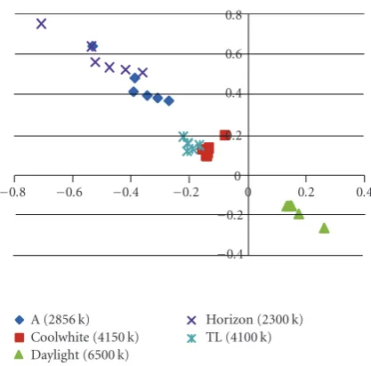
Figure5: Predefined achromatic region (“A” is Incandescent Lamp (CIE-A) and “TL” is Tri- Phosphor Fluorescent (CIE-F11).).
From (12), the directional DGB values are temporary
defined as
DTGBi,j =D
T GBi+m,j+n,
DBGBi,j =D
B GBi+m,j+n,
DLGBi,j =D
L GBi+m,j+n,
DRGBi,j =D
R GBi+m,j+n.
(14)
Using the directional DGR and DGB values and the
assumption dG → 0, DGR ∼= KR, the temporary used
chrominance valuesKRandKBare expressed as
KRi,j= DL
GRi,j+D
R GRi,j
2 DV > DH,
KRi,j=
DTGRi,j+D
B GRi,j
2 DV < DH,
KBi,j =
DL GBi,j+D
R GBi,j
2 DV > DH,
KBi,j =
DT GBi,j+D
B GBi,j
2 DV < DH.
(15)
From (10) and (15), we obtained the luminance and chrominance information that we used to calculate the color constancy gain. Figure 5 shows a predefined achromatic region that prevented a color failure situation when more than one uniform object existed in an image. The predefined achromatic region is obtained using a color chart under different lighting conditions. Using the mean information of the Bayer CFA data, information about the dominant color of the image is obtained and this information restricted the
−0.8 −0.6 −0.4 −0.2 0 0.2 0.4 −0.4
−0.2 0 0.2 0.4 0.6 0.8 1 Achromatic region
Average point
d
(a)
−0.8 −0.6 −0.4 −0.2 0 0.2 0.4 −0.4
−0.2 0 0.2 0.4 0.6 0.8 1 Achromatic region
Average point
(b)
Figure6: Restricted achromatic region: (a) average point inside the achromatic region and (b) average point outside the achromatic region.
predefined achromatic region for accurate color constancy gain. The average point is defined as (G−R)/Gand (G−B)/G. When the distance between the average point and the pre-defined achromatic region is smaller than the prepre-defined thresholdd, the possible achromatic region becomes
CI= p,q
|p−p12+q−q12≤d2, (16)
whereprepresents the abscissa andqrepresents the ordinate. pandqare defined asp=(G−R)/Gandq=(G−B)/Gand (p1,q1) represents a nearest point in the predefined region from the average point. Otherwise, the possible achromatic region becomes
CI=
p,q|p−2d≤p≤p+ 2d,
ap+ (b−d)≤q≤ap+ (b+d), (17)
whereq =ap+brepresents a linear function of the prede-fined region. In this paper,aandb, which are obtained from
Figure 5, are −1.1394 and −0.0068, respectively. Figure 6
explains (16) and (17).
By using the estimated luminance and chrominance information, the color constancy gains are obtained as
KRW=
i,j∈h1,KR/G,KB/G∈CI
KRi,j/Gi,j
N ,
KW
B =
i,j∈h1,KR/G,KB/G∈CI
KBi,j/Gi,j
N ,
33.15 33.2 33.25 33.3 33.35
0 5 10 15 20 25
(a)
1.5 1.6 1.7 1.8 1.9 2
0 5 10 15 20 25
(b)
Figure7: Performance of the proposed algorithm at different settings of thresholdTflat: (a) PSNR and (b) Run Time.
33.15 33.2 33.25 33.3 33.35
0 5 10 15 20 25
(a)
1.5 1.6 1.7 1.8 1.9 2
0 5 10 15 20 25
(b)
Figure8: Performance of the proposed algorithm at different settings of thresholdTedge: (a) PSNR and (b) Run Time.
33.33 33.335 33.34 33.345 33.35 33.355
0 20 40 60 80 100 120 140 160
(a)
33.315 33.325 33.335 33.345 33.355
0 50 100 150 200 250 300 350
(b)
GL i−2,j−2
Gi−1,j−2
GL i,j−2
Gi+1,j−2
GLi+2,j−2
Gi−2,j−1
GL i−1,j−1
Gi−1,j
GL i+1,j−1
Gi+2,j−1
GL i−2,j
GR i−2,j
Gi−1,j
GLi,j
GR i,j
Gi+1,j
GLi+2,j
GRi+2,j
Gi−2,j+1
GR i−1,j+1
Gi,j+1
GR i+1,j+1
Gi+2,j+1
GR i−2,j+2
Gi−1,j+2
GR i,j+2
Gi+1,j+2
GRi+2,j+2
(a)
GTi−2,j−2
Gi−1,j−2
GT i,j−2
GB i,j+2
Gi+1,j−2
GB i+2,j−2
Gi−2,j−1
GTi−1,j−1
Gi−1,j
GB i+1,j−1
Gi+2,j−1
GTi−2,j
Gi−1,j
GT i,j
GBi,j
Gi+1,j
GB i+2,j
Gi−2,j+1
GT i−1,j+1
Gi,j+1
GB i+1,j+1
Gi+2,j+1
GTi−2,j+2
Gi−1,j+2
GTi,j+2
GB i,j+2
Gi+1,j+2
GB i+2,j+2
(b)
DL GRi−2,j−2
Gi−1,j−2
DGRiL ,j−2
Gi+1,j−2
DL GRi+2,j−2
DL GRi−2,j−1
Bi−1,j−1
DL GRi,j−1
Bi+1,j−1
DLGRi+2,j−1
DL GRi−2,j
DR GRi−2,j
Gi−1,j
DL GRi,j
DRGRi,j
Gi+1,j
DL GRi+2,j
DR GRi+2,j
DR GRi−2,j+1
Bi−1,j+1
DRGRi,j+1
Bi+1,j+1
DRGRi+2,j+1
DR GRi−2,j+2
Gi−1,j+2
DRGRi,j+2
Gi+1,j+2
DR GRi+2,j+2
(c)
DT GRi−2,j−2
DT GRi−1,j−2
DGRiT ,j−2
DB GRi,j−2
DGRiB +1,j−2
DB GRi+2,j−2
Gi−2,j−1
Bi−1,j−1
Gi−1,j−1
Bi+1,j−1
Gi+2,j−1
DT GRi−2,j
DT GRi−1,j
DT GRi,j
DB GRi,j
DGRiB +1,j
DB GRi+2,j
Gi−2,j+1
Bi−1,j+1
Gi,j+1
Bi+1,j+1
Gi+2,j+1
DT GRi−2,j+2
DT GRi−1,j−1
DGRiT ,j+2
DGRiB ,j+2
DBGRi+1,j−1
DBGRi+2,j+2
(d)
Figure10: Flat and edge region: (a) left and right for theGchannel, (b) top and bottom for theGchannel, (c) left and right for the
KR channel, and (d) top and bottom for theKRchannel.
whereh1 represents an edge pixel, as defined in (9), andN represents the total number of edge pixels included inCI.
The obtained color constancy gain is used for theRandB channels while the Gchannel demosaicing at the RandB pixel locations.
A detailed explanation will be provided in the next section.
2.3. Green Channel Demosaicing. In a Bayer CFA, the green plane is sampled at a rate twice as high as in the red and blue planes. Thus, the amount of aliasing in the green plane tends to be less than that in the red and blue planes. The green plane possesses the most spatial information of the image to be interpolated and has a great influence on the visual quality
of the image. In most cases, the AWB method alters only the RandBchannels. TheGchannel is kept unchanged because the wavelength of the green color band is close to the peak of the human luminance frequency response. For these reasons, green plane interpolation at theRandBchannels should be performed first.
The estimated values of Gare expressed as a weighted sum of the initial estimateGkandK
Ais expressed using the
result of theGvalues. We express them as
Gi,j=
k∈{T,B,L,R}wkGki,j
k∈{T,B,L,R}wk
,
KAi,j =Gi,j−Ai,j.
GL i−2,j−2
Gi−1,j−2
GLi,j−2
Gi+1,j−2
GLi+2,j−2
Gi−2,j−1
GLi−1,j−1
Gi−1,j
GLi+1,j−1
Gi+2,j−1
GL i−2,j
GRi−2,j
Gi−1,j
GL i,j
GR i,j
Gi+1,j
GL i+2,j
GR i+2,j
Gi−2,j+1
GRi−1,j+1
Gi,j+1
GRi+1,j+1
Gi+2,j+1
GRi−2,j+2
Gi−1,j+2
GRi,j+2
Gi+1,j+2
GRi+2,j+2
(a)
GTi−2,j−2
Gi−1,j−2
GTi,j−2
GB i,j+2
Gi+1,j−2
GB i+2,j−2
Gi−2,j−1
GT i−1,j−1
Gi−1,j
GBi+1,j−1
Gi+2,j−1
GTi−2,j
Gi−1,j
GTi,j
GB i,j
Gi+1,j
GB i+2,j
Gi−2,j+1
GTi−1,j+1
Gi,j+1
GBi+1,j+1
Gi+2,j+1
GTi−2,j+2
Gi−1,j+2
GTi,j+2
GB i,j+2
Gi+1,j+2
GB i+2,j+2
(b)
DL GRi−2,j−2
Gi−1,j−2
DL GRi,j−2
Gi+1,j−2
DLGRi+2,j−2
DL GRi−2,j−1
Bi−1,j−1
DL GRi,j−1
Bi+1,j−1
DLGRi+2,j−1
DL GRi−2,j
DRGRi−2,j
Gi−1,j
DL GRi,j
DGRiR ,j
Gi+1,j
DL GRi+2,j
DRGRi+2,j
DRGRi−2,j+2
Bi−1,j+1
DR GRi,j+1
Bi+1,j+1
DR GRi+2,j+1
DR GRi−2,j+2
Gi−1,j+2
DR GRi,j+2
Gi+1,j+2
DR GRi+2,j+2
(c)
DTGRi−2,j−2
DT GRi−1,j−2
DT GRi,j−2
DBGRi,j−2
DB GRi+1,j−2
DBGRi+2,j−2
Gi−2,j−1
Bi−1,j−1
Gi−1,j−1
Bi+1,j−1
Gi+2,j−1
DTGRi−2,j
DT GRi−1,j
DT GRi,j
DB GRi,j
DB GRi+1,j
DBGRi+2,j
Gi−2,j+1
Bi−1,j+1
Gi,j+1
Bi+1,j+1
Gi+2,j+1
DGRiT −2,j+2
DT GRi−1,j−1
DTGRi,j+2
DBGRi,j+2
DB GRi+1,j−1
DGRiB +2,j+2
(d)
Figure11: Pattern region: (a) left and right for theGchannel, (b) top and bottom for theGchannel, (c) left and right for theKR channel (d), and top and bottom for theKRchannel.
It was found that, in local regions of a natural image, the color differences between the pixels are quite flat [7]. Also, the green channel is flat in homogeneous regions. Accordingly, the variances of Gk and Dk
GA are used as
supplementary information to determine the interpolation direction, where GA is either GR or GB. In order to minimize the directional interpolation error and accurately estimate the direction of interpolation, the weight function is designed inversely proportional to theσ2
Gk value andσD2k GA (wk ∝ 1/σG2k,wk ∝ 1/σD2k
GA). Regardless of the orientation of an edge, at least one of the four estimates is an accurate estimate of the missing green color [24]. To illustrate the above mentioned concept, the weight function is defined
to pick one of the four estimates. In the paper, the weight functionwkis defined as
wk= ⎧ ⎪ ⎪ ⎪ ⎪ ⎪ ⎪ ⎪ ⎪ ⎨ ⎪ ⎪ ⎪ ⎪ ⎪ ⎪ ⎪ ⎪ ⎩ 1, σ 2 Gk TG +σ 2 Dk GA TK =min ⎧ ⎨ ⎩ σ2 Gk TG +σ 2 Dk GA
TK |k∈T,B,L,R ⎫ ⎬
⎭,
0, otherwise,
(20)
where σ2
Gk and σD2k
GA are variances of G
k and Dk
GA. These
variances are calculated in the mask defined in Figures 10
(a) (b) (c) (d)
(e) (f) (g) (h)
Figure12: Partially magnified Kodak 1 image: (a) original image, (b) method discussed in [7], (c) method discussed in [10], (d) method discussed in [15], (e) method discussed in [22], (f) method discussed in [24], (g) method discussed in [27], and (h) Proposed method.
to determine edge directions in the pattern edge region. Therefore, multiple directional rectangular windows are used for the calculation of local statistics to use the directional information of neighboring pixels. On the other hand, a directional rectangular window is used for the calculation of local statistics in the flat and edge regions. TG and TK
represents a predefined thresholds to control the weight of σ2
Gk andσD2k
GA in the weight function. From (18)–(19), white balance processing is written by
Ai,j=Gi,j−
KAi,j−Gi,j×K
W A
, (21)
where KW
A is either KRW and KBW. From (19) and (21), a
fully interpolated G channel and white balanced R andB channels are obtained. Using these values,RandBchannel demosaicing is performed.
2.4. Red and Blue Plane Interpolation. As explained in previous section, the problem of recovering red and blue channels becomes the demosaicing without color constancy problem. Although the red and blue planes are more sparsely sampled than the green planes, they are easily interpolated by using the fully interpolated green plane and theKRandKB
domains. Similar to green plane interpolation, the missingR value at theBlocation is estimated adaptively by
Ri,j=Gi,j−
k,l∈hwRi−k,j−lKiR−k,j−l
k,l∈hwRi−k,j−l
, (22)
where (k,l) = {(−1,−1), (−1, +1), (+1,−1), (+1, +1)}. In this case,KRis calculated directly, using fully interpolatedG
channel values.wis the same value as the one in the green plane, except in a different pixel location. The interpolation of theRvalues at theGlocation and the interpolation of the Bvalues are performed in a similar way as interpolation of theRvalue at theBlocation.
3. Experimental Results
(a) (b) (c) (d)
(e) (f) (g) (h)
Figure13: Partially magnified Kodak 19 image: (a) original image, (b) method discussed in [7], (c) method discussed in [10], (d) method discussed in [15], (e) method discussed in [22], (f) method discussed in [24], (g) method discussed in [27], and (h) Proposed method.
order to measure the performance of the proposed algorithm quantitatively. The PSNR was defined in decibels as
PSNR=10 log10255 2·N
x−x2, (23)
whereNrepresents the total number of pixels in the image, xis the original color image, andxis the demosaiced color image. The NCD is computed in theL∗a∗b∗color space by using the following equation:
NCD=
M
i=1
N
j=1 ΔELab
M
i=1
N
j=1ELab∗
, (24)
whereΔELabis the perceptual color error between two color vectors and is defined as the Euclidean distance between them and is given by
ΔELab=(ΔL∗)2+ (Δa∗)2+ (Δb∗)2b1/2, (25) whereΔL∗,Δa∗, andΔb∗ are the differences in theL∗,a∗, andb∗components. The magnitude of the pixel vector in the L∗a∗b∗of the original image isELab∗ and is given by
E∗Lab=
(L∗)2+ (a∗)2+ (b∗)21/2. (26)
Experiments were also performed on 12-bit sensor data taken from a Micron 2-Megapixel image sensor (MT9D111) in an indoor environment with different lighting conditions and in an outdoor environment. The measurement of the performance of the proposed algorithm was divided into two stages. The first stage is the color demosaicing performance and the second stage is the color constancy ability. In the first stage, for comparison, six conventional algorithms, including the methods of Pei and Tam [7], Hamilton and Adams [10], Lu and Tan [15], Wu and Zhang [22], Li and Randhawa [24], and Tsai and Song [27], were implemented. In the second stage, the proposed algorithms were compared with the results of GW, Max-RGB, Shades of Gray, and Gray edge [30].
For the proposed method, an empirical study was carried out to select an appropriate threshold value ofTedge,Tflat, TG, and TK. Figures7 and8 illustrate the performance of the proposed algorithm at difference settings of threshold Tflat and Tedge. From Figure 7, the optimal choice of the thresholdTflatis 10. When the thresholdTflatis 10, the PSNR value is the largest and the run time does not change much after 10. FromFigure 8, the optimal choice of the threshold Tedge is set to 10. In the test image set,σ2
G is about 4 times
bigger thanσ2
(a) (b)
(c) (d)
(e) (f)
Figure14: Result of the AWB method: (a) Kodak 1 image, (b) Gray world, (c) Max-RGB, (d) Shades of Gray, (e) Gray Edge, and (f) Proposed method.
TK.Figure 9does not show serious numerical differences at
difference settings of thresholdTGandTK. In this paper,TG
andTK are set to 120 and 30, respectively, to balance the
effect ofσ2
Gk andσD2k
GA in the weight function.The threshold d in (16) and (17) is determined using Figure 5. In the experiments, 0.25 is used as the thresholdd.
Tables 1 and 2 show some numerical comparisons of the color demosaicing method. In each table, the bold font denotes the largest PSNR and smallest NCD values across each image. From Tables1 and2, the proposed algorithm provides the improved PSNR and NCD values in most of the test images. In the case of fairly flat images, the proposed
(a) (b)
(c) (d)
(e) (f)
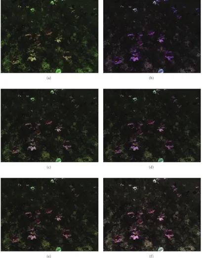
Figure15: Result of the AWB method: (a) original image, (b) Gray world, (c) Max-RGB, (d) Shades of Gray, (e) Gray Edge, and (f) Proposed method.
most of the test images. Although the proposed method did not provide the best PSNR and NCD results for several images, it outperformed the other algorithms.
To evaluate the proposed method, the visual quality of the test image was compared numerically, and also with some conventional methods. Figures12and13contain eight partially magnified images: the original Kodak images and
the resulting images obtained by the methods proposed by Pei and Tam [7], Hamilton and Adams [10], Lu and Tan [15], Wu and Zhang [22], Li and Randhawa [24], and Tsai and Song [27], and the proposed method.
(a) (b)
(c) (d)
(e) (f)
Figure16: Result of the AWB method: (a) original image, (b) Gray world, (c) Max-RGB, (d) Shades of Gray, (e) Gray Edge, and (f) Proposed method.
is clear that most conventional methods suffered from zipper effects along the edges. The methods proposed by Wu and Zhang, Li and Randhawa, and Tsai and Song showed good results but they still produce more color artifacts than the proposed method. These experimental results explain that the proposed method performs satisfactorily not only in textured regions but also in normal edge regions.
Table 3 shows the numerical comparisons of a
con-ventional AWB method and the proposed method. The √
Cb2+Cr2value was calculated in the achromatic region of the color chart image. The smaller the value of√Cb2+Cr2, the better the algorithm should have been [31]. As shown in Table 3, the proposed algorithm provided an improved √
Table1: PSNR comparison of color demosaicing algorithms.
Method [7] [10] [15] [22] [24] [27] Proposed method
1 29.139 26.237 31.374 31.281 30.959 30.147 32.773
2 33.942 31.958 34.431 35.164 34.625 32.996 35.111
3 36.174 33.735 36.169 37.172 36.740 33.789 37.533
4 35.209 32.674 35.060 35.076 34.537 32.838 35.775
5 30.638 27.599 32.420 32.029 31.532 30.506 32.772
6 30.162 27.736 32.124 33.303 33.604 32.014 34.702
7 35.758 33.462 36.182 36.670 36.349 32.854 36.866
8 25.955 24.015 29.597 29.644 28.863 28.525 30.643
9 34.863 32.778 35.917 37.301 36.767 33.109 37.550
10 35.450 32.795 36.159 36.752 36.093 32.988 37.204
11 31.713 29.171 33.284 33.650 33.367 31.434 34.647
12 35.046 33.0381 36.2903 37.4469 37.5518 32.7008 37.976
13 26.693 23.301 27.819 27.701 27.634 26.955 29.285
14 30.959 28.983 32.244 32.065 31.426 30.725 31.887
15 33.102 30.691 33.646 34.212 33.156 32.402 34.351
16 33.372 31.055 34.760 36.921 37.511 34.146 38.281
17 34.689 31.582 35.320 35.622 35.301 33.022 36.581
18 30.506 27.321 30.943 31.107 30.569 29.939 31.694
19 30.596 28.750 33.310 34.601 34.118 31.762 35.460
20 33.982 31.155 33.660 35.107 34.540 33.681 35.652
21 31.137 28.393 31.977 32.499 32.310 30.552 33.778
22 32.021 30.007 32.333 32.969 32.552 30.839 33.157
23 37.170 34.873 36.444 37.873 37.225 34.0518 37.916
24 28.879 25.819 28.550 29.437 28.574 28.794 30.205
Average 32.381 29.880 33.334 33.983 31.699 33.579 34.658
the average√Cb2+Cr2 was compared, the proposed algo-rithm improved from about 0.3 to about 1.5.
For evaluating the results, numerical comparisons were important, and so was a the visual quality comparison. Figures14–16contain six images the original images and the resulting images obtained by the GW methods, max-RGB, Shades of Gray, Gray edge [30], and the proposed method. The conventional AWB methods were obtained by using the proposed color demosaicing method because this was the first attempt to combine two methods.Figure 14shows the results of the Kodak 1 test image. Most edge regions existed in the wall; so it proved difficult to get a well-whited-balanced image when using the gray edge method. Also, the GW method showed a bluish image due to the dominant color problem. However, the proposed method avoided the dominant color problem because it used a predefined achromatic region and showed a white-balanced image. In Figures15 and16, the results of the real image taken from the Micron 2-megapixel image sensor (MT9D111) (in which the dominant color problem appears) can be seen. There are many objects such as flowers, leaves, grass, and the ground
in the image. These objects have uniform colors and are dispersed in the image; so again, it was difficult to get a well-white-balanced image. The proposed method was able to deal with cases where there were many uniform objects in an image.
To show the computational efficiency of the proposed method, the average run times are presented inTable 4. The experiment was performed on a PC equipped with 3.2 GHz CPU and 4 GB RAM. When computational complexity was compared with the cascade color demosaicing method and the AWB algorithm, the proposed method improved efficiency by about 10%.
4. Conclusions
Table2: NCD comparison of color demosaicing algorithms.
Method [7] [10] [15] [22] [24] [27] Proposed method
1 3.3642 4.8614 2.4648 2.5723 2.5855 2.6255 2.0038
2 2.3222 2.8759 1.9663 2.0716 2.0967 2.0942 2.0186
3 1.4192 1.9295 1.2932 1.3320 1.3249 1.3996 1.2512
4 1.7575 2.4308 1.6365 1.7548 1.8524 1.8983 1.6150
5 4.2188 5.5268 3.0787 3.4729 3.6039 3.6878 3.0593
6 2.3901 3.3519 1.8369 1.6963 1.5771 1.731 1.4103
7 1.6883 2.1963 1.4123 1.5237 1.5247 1.6259 1.4994
8 4.0698 5.3445 2.6195 2.6783 2.7872 2.8475 2.2732
9 1.3281 1.8437 1.1006 1.0799 1.0946 1.2112 1.0030
10 1.2920 1.8610 1.1320 1.1782 1.1866 1.3199 1.0792
11 3.0053 3.9284 2.2764 2.3406 2.3375 2.4373 2.0996
12 1.0234 1.4854 0.8695 0.8450 0.8295 0.9139 0.7744
13 4.7222 6.9852 3.9882 4.2398 4.2848 4.2964 3.2278
14 3.2396 4.1906 2.5953 2.7794 2.8446 2.9388 2.6094
15 2.2142 2.9346 2.0149 2.0663 2.2075 2.1600 2.0052
16 2.1635 2.9721 1.6778 1.4987 1.3683 1.5698 1.2589
17 2.6429 3.5263 2.2175 2.3417 2.4115 2.5657 2.1226
18 4.1882 5.7475 3.8332 3.8676 4.2533 4.1030 3.7728
19 2.4973 3.4972 1.9400 1.8843 1.9515 2.0023 1.6513
20 1.4892 2.0914 1.3428 1.3168 1.3752 1.3550 1.1949
21 2.3918 3.3835 1.9527 2.0638 2.0501 2.1609 1.6947
22 2.1328 2.9178 1.9437 2.0020 2.0905 2.1126 1.9271
23 1.2644 1.5910 1.2928 1.2699 1.3045 1.3572 1.2883
24 2.5183 3.4042 2.1787 2.2341 2.3844 2.3264 2.0180
Average 2.4726 3.36988 2.0277 2.0879 2.1975 2.1386 1.8691
Table3: The average√Cb2+Cr2of a checker board image under six different color temperature light sources.
Before AWB GW Max-RGB SG GE Proposed method
A (2856K) 27.2081 1.0732 3.1478 1.0486 1.0083 0.6997
Coolwhite (4150K) 27.4791 1.0535 1.0803 0.9990 1.0057 0.7731 Daylight (6500K) 23.4127 0.9412 1.0961 0.9463 1.0466 0.7197 Horizon (2300K) 31.7124 1.2960 4.0441 1.2662 1.4153 0.8413
Tl (4100K) 19.5384 0.9778 2.4763 0.9351 0.9490 0.7058
Outdoor 25.5908 2.0421 1.7281 1.0986 0.9233 0.6822
Average 25.8236 1.2306 2.2621 1.0490 1.0580 0.7370
Table4: The computational complexity comparison.
Color demosaicing
Edge based AWB
Proposed method Average running
time (sec) 3.404 0.44 3.486
estimates were calculated for AWB weight and color demo-saicing by using second-order Taylor series approximation and an SSC assumption. The gray edge assumption was used to achieve color constancy and a predefined achromatic region was used to avoid dominant color problem. Region adaptive color demosaicing was performed to improve the
Acknowledgments
This work was supported in part by the National Research Foundation of Korea (NRF) grant funded by the Korea government (MEST) through the Biometrics Engineer-ing Research Center (BERC) at Yonsei University (2009-0062990) and by Basic Science Research Program through the National Research Foundation of Korea (NRF) funded by the Ministry of Education, Science and Technology (2009-0079024).
References
[1] B. E. Bayer, “Color imaging array,” US patent 3 971 065, July 1976.
[2] D. Forsyth, “A novel algorithm for color constancy,” Interna-tional Journal of Computer Vision, vol. 5, no. 1, pp. 5–36, 1990. [3] D. R. Cok, “Signal processing method and apparatus for producing interpolated chrominance values in a sampled color image signal,” US patent 4 642 678, Febraury 1987.
[4] J. E. Adams Jr., “Interactions between color plane interpola-tion and other image processing funcinterpola-tions in electronic pho-tography,” inCameras and Systems for Electronic Photography and Scientific Imaging, vol. 2416 ofProceedings of SPIE, pp. 144–151, San Jose, Calif, USA, February 1995.
[5] J. E. Adams and J. F. Hamilton Jr., “Adaptive color plane interpolation in single color electronic camera,” US patent 5 506 619, April 1996.
[6] J. E. Adams Jr., “Design of practical color filter array interpola-tion algorithms for digital cameras,” inReal-Time Imaging II, vol. 3028 ofProceedings of SPIE, pp. 117–125, San Jose, Calif, USA, February 1997.
[7] S.-C. Pei and I.-K. Tam, “Effective color interpolation in CCD color filter arrays using signal correlation,”IEEE Transactions on Circuits and Systems for Video Technology, vol. 13, no. 6, pp. 503–513, 2003.
[8] R. H. Hibbard, “Apparatus and method for adaptively inter-polating a full color image utilizing luminance gradients,” US patent 5 382 976, January 1995.
[9] C. A. Laroche and M. A. Prescott, “Apparatus and method for adaptively interpolating a full color image utilizing chromi-nance gradients,” US patent 5 373 322, December 1994. [10] J. F. Hamilton Jr. and J. E. Adams, “Adaptive color plane
interpolation in single sensor color electronic camera,” US patent 5 629 734, May 1997.
[11] J. E. Adams Jr. and J. F. Hamilton Jr., “Adaptive color plane interpolation in single sensor color electronic camera,” US patent 5 652 621, July 1997.
[12] R. Kimmel, “Demosaicing: image reconstruction from color CCD samples,”IEEE Transactions on Image Processing, vol. 8, no. 9, pp. 1221–1228, 1999.
[13] B. S. Hur and M. G. Kang, “Edge-adaptive color interpolation algorithm for progressive scan charge-coupled device image sensors,”SPIE Optical Engineering, vol. 40, no. 12, pp. 2698– 2708, 2001.
[14] S. W. Park and M. G. Kang, “Color interpolation with variable color ratio considering cross-channel correlation,”
SPIE Optical Enginerring, vol. 43, no. 1, pp. 34–43, 2004. [15] W. Lu and Y. Tan, “Color fiter array demosaicking: new
method and performance measures,” IEEE Transactions on Image Processing, vol. 12, no. 10, pp. 1194–1210, 2003. [16] R. Ramanath and W. E. Snyder, “Adaptive demosaicking,”
Journal of Electronic Imaging, vol. 12, no. 4, pp. 633–642, 2003.
[17] C. Kim and M. G. Kang, “Noise insensitive high resolution color interpolation scheme considering cross-channel corre-lation,”SPIE Optical Engineering, vol. 44, no. 12, Article ID 127006, 15 pages, 2005.
[18] H. Trussel and R. Hartwig, “Mathematics for demosaicking,”
IEEE Transactions on Image Processing, vol. 11, pp. 485–492, 2002.
[19] D. Keren and M. Osadchy, “Restoring subsampled color images,”Machine Vision Applied, vol. 11, no. 4, pp. 197–202, 1999.
[20] B. K. Gunturk, Y. Altunbasak, and R. M. Mersereau, “Color plane interpolation using alternating projections,”IEEE Trans-actions on Image Processing, vol. 11, no. 9, pp. 997–1013, 2002. [21] J. Mukherjee, R. Parthasarathi, and S. Goyal, “Markov random field processing for color demosaicing,”Pattern Recognition Letters, vol. 22, no. 3-4, pp. 339–351, 2001.
[22] X. L. Wu and N. Zhang, “Primary-consistent soft-decision color demosaicking for digital cameras (patent pending),”
IEEE Transactions Processing, vol. 13, no. 9, pp. 1263–1274, 2004.
[23] K. Hirakawa and T. W. Parks, “Adaptive homogeneity-directed demosaicing algorithm,”IEEE Transactions on Image Process-ing, vol. 14, no. 3, pp. 360–368, 2005.
[24] J. S. J. Li and S. Randhawa, “High order extrapolation using taylor series for color filter array demosaicing,” in
Proceedings of the International Conference on Image Analysis and Recognition (ICIAR ’05), vol. 3656 of Lecture Notes in Computer Science, pp. 703–711, Toronto, Canada, September 2005.
[25] L. Zhang and X. Wu, “Color demosaicking via directional linear minimum mean square-error estimation,”IEEE Trans-actions on Image Processing, vol. 14, no. 12, pp. 2167–2178, 2005.
[26] K.-H. Chung and Y.-H. Chan, “Color demosaicing using variance of color differences,” IEEE Transactions on Image Processing, vol. 15, no. 10, pp. 2944–2955, 2006.
[27] C.-Y. Tsai and K.-T. Song, “Heterogeneity-projection hard-decision color interpolation using spectral-spatial correla-tion,”IEEE Transactions on Image Processing, vol. 16, no. 1, pp. 78–91, 2007.
[28] K. Barnard, V. Cardei, and B. Funt, “A comparison of com-putational color constancy algorithms—part I: methodology and experiments with synthesized data,”IEEE Transactions on Image Processing, vol. 11, no. 9, pp. 972–984, 2002.
[29] K. Barnard, L. Martin, A. Coath, and B. Funt, “A compar-ison of computational color constancy algorithms—part II: experiments with image data,” IEEE Transactions on Image Processing, vol. 11, no. 9, pp. 985–996, 2002.
[30] J. van de Weijer, T. Gevers, and A. Gijsenij, “Edge-based color constancy,”IEEE Transactions on Image Processing, vol. 16, no. 9, pp. 2207–2214, 2007.
[31] J. Lin, “An automatic white balance method based on edge detection,” in Proceedings of the 10th IEEE International Symposium on Consumer Electronics (ISCE ’06), pp. 1–4, 2006. [32] E. Land and J. McCann, “Lightness and retinex theory,”
Journal of the Optical Society of America A, vol. 61, no. 1, pp. 1–11, 1971.
[33] G. D. Finlayson, S. D. Hordley, and I. Tastl, “Gamut constrained illuminant estimation,”International Journal of Computer Vision, vol. 67, no. 1, pp. 93–109, 2006.
[35] G. D. Finlayson, S. D. Hordley, and P. M. Hubel, “Color by cor-relation: a simple, unifying framework for color constancy,”
IEEE Transactions on Pattern Analysis and Machine Intelligence, vol. 23, no. 11, pp. 1209–1221, 2001.